Introduction
This paper grew out of an investigation of automorphisms of spherical buildings with very restricted displacement spectra. In a series of papers, the second author, often jointly with various co-authors, among mainly James Parkinson, described — and in many cases classified — automorphisms of Moufang spherical buildings that do not map chambers to opposite ones. This analysis showed that the case in which the automorphism also does not fix any chamber (as a kind of “dual” or “complementary” condition to the condition of not mapping a chamber to one at maximal distance) is rather special. Only automorphisms with a rich fix structure turned up. Eliminating those fixed point structures that do not correspond to fix diagrams lead to the notion of uniclass automorphisms. These are automorphisms of buildings whose displacement spectra is contained in a unique (twisted) conjugacy class of the Weyl group of the building. It turned out that an automorphism of a spherical building is uniclass if, and only if, its fix structure is a well defined given substructure of the building, see [17]. These substructures were defined type by type and the only link between different structures was noted through the Freudenthal–Tits Magic Square, where most of the fix and opposition diagrams in the exceptional cases occur in a structured way. However, many Weyl substructures can not be linked with this magic square, such as the Ree–Tits octagons, which occur as fixed point sets of polarities in buildings of type \(\mathsf{F_4}\) and these polarities are uniclass. In the present paper, we provide a uniform combinatorial definition of Weyl substructure across all types in an axiomatic way, connecting previously seemingly unrelated geometric substructures in different spherical buildings. Roughly, our object — which we will call an ovoidal subcomplex, because we use the viewpoint of simplicial complexes for buildings — is a convex numbered subcomplex satisfying a simple residual property (see below for details). However, since the convexity condition is not always easy to check, we prove that a weaker condition suffices. Reviewing the different types of spherical buildings, we will see that we can even sometimes completely ignore any convexity condition, or use a very weak one like the exclusion of a certain mutual position between any pair of vertices of a given type of the subcomplex. As the name suggests, the defining residual property of an ovoidal subcomplex uses the notion of an ovoid of a polar space, one of the most fundamental combinatorial notions in (mostly finite) geometry. Let us now provide some more details.
In [17] we defined a Weyl substructure of a spherical building by the following list of geometries in the corresponding point-line geometries, mentioned between parentheses, defined by the spherical buildings in question. Each Weyl substructure is a spherical subbuilding, and its type is called the relative type. We also assign a class number, which is the order of the automorphism of the Coxeter graph induced by the automorphism of the building that is intended to fix the given substructure. For the precise definition of each substructure, we refer to the relevant section in the paper.
- (1) The full building;
- (2) In type \(\mathsf{A}_n\) (projective space, \(n\) always odd, definitions in Subsection 4.1):
- (a) The standard symplectic polar space; relative type \(\mathsf{B}_{(n+1)/2}\), class 2.
- (b) A composition line spread; relative type \(\mathsf{A}_{(n-1)/2}\), class 1.
- (3) In type \(\mathsf{B}_n\) or \(\mathsf{D}_n\) (general polar spaces, definitions in Subsection 4.3):
- (a) An ideal subspace of corank \(i\); relative type \(\mathsf{B}_{n-i}\), class \(2\) if \(i\) is odd and the type is \(\mathsf{D}_n\), class \(1\) otherwise.
- (b) A composition line spread; relative type \(\mathsf{B}_{n/2}\), class 1.
- (4) Type \(\mathsf{E}_6\) (definitions in Subsection 4.4):
- (a) The standard embedded split metasymplectic space; relative type \(\mathsf{F_4}\), class 2.
- (b) An ideal Veronesian; relative type \(\mathsf{A}_2\) (projective plane over quaternion or octonion division algebra), class 1.
- (5) Type \(\mathsf{E}_7\) (definitions in Subsection 4.6):
- (a) An ideal fully embedded metasymplectic space (which is then quadratic and either has absolute type \(\mathsf{E_6}\) or is inseparable); relative type \(\mathsf{F}_4\), class 1.
- (b) An ideal dual polar (quaternion) Veronesian; relative type \(\mathsf{B}_3\), class 1.
- (6) Type \(\mathsf{E}_8\) (definitions in Subsection 4.7):
- (a) An ideal fully embedded metasymplectic space (which is then quaternion and either has absolute type \(\mathsf{E_7}\) or is inseparable); relative type \(\mathsf{F}_4\), class 1.
- (7) Type \(\mathsf{F}_4\) (metasymplectic space, definitions in Subsection 4.5):
- (a) A flat and linear ideal quadrangular Veronesian; relative type \(\mathsf{B}_2\), class 1.
- (b) A Ree-Tits octagon; relative type \(\mathsf{I_2}(8)\), class 2.
- (8) Type \(\mathsf{I_2}(n)\) (generalized polygons, \(n\) always even, definitions in Subsection 4.2):
- (a) An ovoid or a spread; relative type \(\mathsf{A}_1\), class 1.
- (b) An ovoid-spread pairing; relative type \(\mathsf{A_1}\), class 2.
A special case of (3)(a) is a parabolic subquadric of rank \(n\) in a hyperbolic quadric of rank \(n+1\), arising as a (non-degenerate) hyperplane section. In the present paper, we define an ovoidal subcomplex of a spherical building, roughly as follows: it is a numbered subcomplex (where the numbering respects the symmetry of the diagram, see below) such that the residue of every panel in the whole building is the spherical building defined by the direct product of polar spaces (including rank 1) and generalized polygons, and its residue in the subcomplex represents either an ovoid in exactly one component of that direct product, or an ovoid-spread pairing in a generalized polygon residue (including generalised digons). Consider the following weak convexity condition on a subcomplex \(\Sigma\).
(WCC) The convex closure of \(\Sigma\) does not contain simplices of type distinct from each type of the members of \(\Sigma\).
Referring to the first paragraph of Subsection 4.5 for the definition of inseparable building of type \(\mathsf{F_4}\), our first main result then reads:
Main Result 1.1. An ovoidal subcomplex of an irreducible thick spherical building that is not an inseparable building of type \(\mathsf{F_4}\), and which satisfies condition (WCC), is a Weyl substructure (in particular, it is convex). Conversely, every Weyl substructure that is the fix structure of an automorphism, is a convex ovoidal subcomplex.
The weak convexity condition can in general be relaxed, and even deleted for certain types, like type \(\mathsf{A}_n\) and \(\mathsf{E_6}\). We will come back to this and be more precise in Section 4.
The inseparable buildings of type \(\mathsf{F_4}\) are true exceptions and we refer to Remark 4.31 for more details. The reason for their exceptional behaviour is perhaps that they are the unique class of spherical buildings of rank at least \(3\) of “mixed type”, see [32, §2.5]. Main Result 1.1 yields an improvement over [17] for separable buildings of type \(\mathsf{F_4}\) in that we get rid of the extra conditions of flatness and linearity for ideal quadrangular Veroneseans: they are automatically satisfied (and every counterexample in the inseparable case is not flat or linear), see Subsection 4.5.
The property of a convex subcomplex of being “ovoidal” expresses a certain maximality in size among subcomplexes of the same type, as ovoids are the maximal subcomplexes of polar spaces of rank 1 consisting of points. However, also spreads of maximal singular subspaces in polar spaces of rank at least 3 (and also simple spreads in projective spaces of dimension at least 5) are large maximal subcomplexes of rank 1 and yet do not appear as Weyl substructure. We elaborate on this in Section 5, where we show that each Weyl substructure has dimension at least half of the dimension of its corresponding natural variety, see Observation 5.1.
We also note that Main Result 1.1 yields a new characterisation of the Ree–Tits octagons as embedded octagons in metasymplectic spaces, see Theorem 4.33.
Let \(\Delta\) be a spherical building with Coxeter system \((W,S)\). Let \(\theta\) be an automorphism of \(\Delta\), and let \(\sigma\) be its companion diagram automorphism (see Subsection 2.2 for precise definitions or references). Denote by \(\delta\) the \(W\)-valued distance function defined on the set of chambers of \(\Delta\) (and we denote that set also with \(\Delta\)). The displacement spectra of \(\theta\) is \[\mathop{\mathrm{\mathsf{Disp}}}(\theta)=\{\delta(C,C^{\theta})\mid C\in\Delta\}.\]
If \(\Delta\) is thin (that is, a Coxeter complex) then it is easy to see that \(\mathop{\mathrm{\mathsf{Disp}}}(\theta)\) consists of a single \(\sigma\)-conjugacy class in \(W\). That is, \(\mathop{\mathrm{\mathsf{Disp}}}(\theta)=\{u^{-1}wu^{\sigma}\mid u\in W\}\) for some \(w\in W\). In the present paper, we shall refer to a type preserving automorphism of a spherical building as a collineation, and to one that induces an involution on the the diagram, a duality.
We call \(\theta\) uniclass if \(\mathop{\mathrm{\mathsf{Disp}}}(\theta)\) is contained in a single \(\sigma\)-conjugacy class. For example, anisotropic automorphisms (mapping all chambers to opposite chambers) are uniclass. Our second Main Result is a further sharpening of Theorem 1 in [17]. In the latter theorem, the uniclass automorphisms that are not type preserving all turned out to be dualities. For the converse, we required in the duality case that the automorphism was indeed a duality and had order \(2\). In the present paper, we show that we can delete these conditions (but keeping the condition that it pointwise fixes a Weyl substructure). We obtain a short and elegant characterisation of the uniclass automorphisms.
Main Result 1.2. An automorphism of an irreducible spherical building \(\Delta\), assumed not to be type preserving if \(\Delta\) is an inseparable building of type \(\mathsf{F_4}\), is uniclass if, and only if, it is either anisotropic, or if it pointwise fixes a Weyl substructure if, and only if, it is either anisotropic or it pointwise fixes an ovoidal subcomplex satisfying (WCC). In particular, if an automorphism pointwise fixes a Weyl substructure of class \(2\), which contains vertices that are simplices of dimension at least \(2\) of \(\Delta\), then it is either the identity, or it is a polarity.
The hard work in showing that an arbitrary automorphism fixing a given Weyl substructure of class 2 is a polarity occurs for type \(\mathsf{F_4}\). However, in this case, we prove a slightly stronger result, which we now state, as it is of independent interest.
Proposition 1.3. Let \(A\) be the set of absolute points of a polarity \(\rho\) of a building of type \(\mathsf{F_4}\). Then every duality for which every point of \(A\) is absolute coincides with \(\rho\). Also, every collineation pointwise fixing \(A\) is the identity.
Table 1. Fix diagrams of non-trivial uniclass automorphisms| Type | Weyl substructure | Symbol | Diagram |
|---|
| \(\mathsf{A}_{2n+1}\) | Symplectic polar space | \({}^2\mathsf{A}_{2n+1;n+1}^{1}\) |

|
| Composition line spread | \(\mathsf{A}_{2n+1;n}^{2}\) |

|
| \(\mathsf{B}_{n}\) | Ideal subspace of corank \(i\) | \(\mathsf{B}_{n;n-i}^{1}\) |

|
| \(\mathsf{B}_{2n}\) | Composition line spread | \(\mathsf{B}_{2n;n}^{2}\) |

|
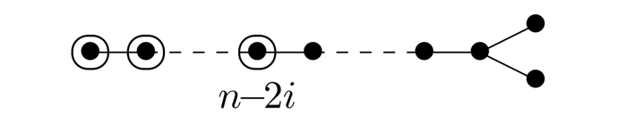
| Ideal subspace of corank \(2i\) | \(\mathsf{D}_{n;n-2i}^{1}\) |
|
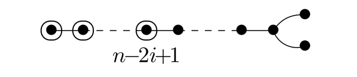
| \(\mathsf{D}_{n}\) | Ideal subspace of corank \(2i-1\) | \(\mathsf{D}_{n;n-2i+1}^{1}\) |
|
| Parabolic quadric of rank n-1 | \(\mathsf{D}_{n;n-1}^{1}\) |

|
| \(\mathsf{D}_{2n}\) | Composition line spread | \(\mathsf{D}_{2n;n}^{2}\) |

|
| \(\mathsf{E}_{6}\) | Metasymplectic space | \({}^2\mathsf{E}_{6;4}\) |

|
| Ideal Veronesean | \(\mathsf{E}_{6;2}\) |

|
| \(\mathsf{E}_{7}\) | Ideal dual polar Veronesean | \(\mathsf{E}_{7;3}\) |

|
| Partial composition spread | \(\mathsf{E}_{7;4}\) |

|
| \(\mathsf{E}_{8}\) | Metasymplectic space | \(\mathsf{E}_{8;4}\) |

|
| \(\mathsf{F}_{4}\) | Ideal quadrangular Veronesean | \(\mathsf{F}_{4;2}\) |

|
| Ree-Tits octagon | \({}^2\mathsf{F}_{4;2}\) |

|
| \(\mathsf{I}_{2}^{(2m)}\) | Ovoid or spread | \(\mathsf{I}_{2;1}^{1}(2m)\) |

|
| Ovoid-spread pairing | \({}^2\mathsf{I}_{2;1}(2m)\) |

|
Note that \(A\) is the point set of a Ree–Tits octagon.
One could also ask whether there exist dualities or, more general, other non type preserving automorphisms pointwise fixing a Weyl substructure \(\Sigma\) of class 1. Then, obviously, the types of the members of \(\Sigma\) must be invariant under the opposition relation. Scrolling through the list below reveals that this only happens in the case of type \(\mathsf{D}_n\) (noting \(\mathsf{A_{3;1}^2=D_{3;1}^1}\)), where the results are all proved in the polar space language, which makes no distinction between collineations and dualities. Hence we do not have to worry about this phenomenon; it has already been taken care of in [17].
Table 1 presents the fix diagrams of non-trivial uniclass automorphisms.
Every uniclass automorphism \(\theta\) comes with a fix diagram, which simply encodes the types of minimal flags being fixed by \(\theta\). We display these fix diagrams in Table 1 for each non-trivial Weyl substructure. On the other hand, an ovoidal subcomplex is numbered, and so we can also speak of the types of the minimal flags it contains. Encircling the corresponding nodes of the diagram, we obtain the Weyl diagram of the ovoidal subcomplex. Our first task is to show that every such Weyl diagram is an existing fix diagram of some uniclass automorphism; hence that the set of Weyl diagrams coincides with the set of fix diagrams of uniclass automorphisms. Independent from the existence of ovoidal subcomplexes with given Weyl diagram, we can define a Weyl diagram as follows.
Firstly, to fix terminology, a Weyl diagram will consist of a spherical Coxeter diagram with a number of distinguished orbits under a common symmetry group of order at most \(2\). These orbits are referred to as the isotropic orbits. Now, a simple Weyl diagram is a spherical Coxeter diagram with exactly one isotropic orbit that either represents the point set of a polar space diagram (when the orbit is a single vertex; this includes the rank 1 case), or is the full orbit of a group of order \(2\) on the diagram of a generalized \(2n\)-gon, \(n\geq 1\). Then, in general, a Weyl diagram is a spherical Coxeter diagram with a number of isotropic orbits, say \(k\), ordered in such a way that the residue diagram of any \(k-1\) of them is the disjoint union of a single simple Weyl diagram and other diagrams (naturally, with no further isotropic orbits). Here, \(k\) is allowed to be zero, in which case we speak of an empty Weyl diagram. By convention, the symmetry group of every empty Weyl diagram is generated by the opposition relation on the types. If \(k=n\), the rank of the Coxeter diagram, then we call it a full Weyl diagram.
Pictorially, we represent a Weyl diagram as the underlying Coxeter diagram with the isotropic orbits encircled.
Main Result 1.4. The set of Weyl diagrams coincides with the set of fix diagrams of uniclass automorphisms of (thick) spherical buildings.
A Weyl diagram will be said to be of class \(1\) if the corresponding group acting on the type set is trivial; otherwise it is of class \(2\). As a consequence, for instance, an empty Weyl diagram is of class 1 if, and only if, the opposition relation acts trivially on the types.
A simple ovoidal subcomplex is one with a simple Weyl diagram. It is always an ovoid in a polar space (including rank 1), or an ovoid-spread pairing of a generalized polygon (including generalised digons).
An additional motivation to explicitly determine all Weyl diagrams is given by possible generalisation of our classification of uniclass automorphisms. Indeed, the definition of Weyl diagram allows generalisation to all Coxeter diagrams, and it is very likely (and we conjecture) that uniclass automorphisms in non-spherical buildings have fix diagrams that are Weyl diagrams. This would already be a very good starting point to investigate uniclass automorphisms in general non-spherical buildings.
There is a subtlety that should be realised. Not all Weyl substructures admit a non-trivial pointwise stabiliser, and it seems impossible to axiomatise geometrically exactly those that do. If we call a Weyl substructure rigid if its full pointwise stabiliser is the trivial group, then, for instance, there exist rigid composition line spreads in certain projective spaces, see [37]. These are a kind of pariahs, satisfying the axioms, but not admitting a group that defines them via its fix structure. When the Weyl substructure has rank \(1\), then it might also be rigid. For instance, an arbitrary ovoid in a generalised quadrangle \(\Gamma\) forms an ovoid-spread pairing with every spread of \(\Gamma\), but if we choose the ovoid or spread not to be related to a polarity, then the ovoid-spread pairing is rigid. An example is the classical ovoid of the symplectic quadrangle over a finite field of characteristic \(2\) of size at least \(8\), which is never an ovoid associated to a polarity, see Chapter 7 of [35]. Other examples occur in infinite polar spaces: one can construct ovoids using a transfinite free induction process, and the resulting ovoids have zero probability of being non-rigid, see [3]. All in all, disregarding the relative rank 1 case, the following theorem seems to confirm that the existence of rigid Weyl substructures is rather a characteristic \(2\) phenomenon. It lists the cases where we know that rigid examples do not exist.
Main Result 1.5. A Weyl substructure, or equivalently, a convex ovoidal subcomplex \(\Sigma\) of a spherical building \(\Delta\) is always the fixed point complex of a non-trivial automorphism of \(\Delta\) in the following cases.
- (i) \(\Delta\) has type \(\mathsf{D}_n\), \(n\geq 4\), \(\mathsf{E_7}\) or \(\mathsf{E_8}\), or
- (ii) \(\Delta\) has type \(\mathsf{A}_{2n}\), \(\mathsf{E_6}\) or \(\mathsf{F_4}\), and \(\Sigma\) is (in all three cases) of class \(2\), or
- (iii) \(\Delta\cong\mathsf{A}_n(\mathbb{K})\), with \(\mathbb{K}\) commutative and \(\mathop{\mathrm{\mathsf{char}}}\mathbb{K}\neq 2\), and \(\Sigma\) is of class \(1\), or
- (iv) \(\Delta\cong\mathsf{E_{6}}(\mathbb{K})\), with \(\mathop{\mathrm{\mathsf{char}}}\mathbb{K}\neq 2\), and \(\Sigma\) is of class \(1\), or
- (v) \(\Delta\) has type \(\mathsf{B}_n\), \(n\geq 3\), \(\Sigma\) has Weyl diagram \(\mathsf{B}_{n;i}^1\), \(2\leq i\leq n-1\) and the polar space associated to \(\Delta\) has, up to isomorphism, a unique embedding in projective space (which is automatic if we are not in characteristic \(2\) here), or
- (vi) \(\Delta\) is a separable building of type \(\mathsf{F_4}\), and \(\Sigma\) is of class \(1\).
Note that the comment between parentheses in (v) makes sense since the (thick) non-embeddable polar spaces do not admit ovoidal subcomplexes with Weyl diagram \(\mathsf{B_{3;2}^1}\), see the comments in the \(\mathsf{B}_n\) paragraph of Section 5.
Structure of the paper
Since, in [17], Weyl substructures are defined in certain Lie incidence geometries associated to spherical buildings, we introduce and review the basics of Lie incidence geometries in Section 2. However, the properties that we need of some specific Lie incidence geometries are recalled when we need them, that is, in the various subsections of Section 4. We will occasionally refer to certain fix and opposition diagrams, so we provide a short introduction in Subsection 2.2. Since Weyl substructures are intimately related to uniclass automorphisms, it seems appropriate to also introduce these; this is also done in Subsection 2.2.
In Section 3 we prove Main Result 1.4. From then on, we can speak of the type of Weyl diagram of an ovoidal subcomplex, and this allows for considering type by type, and it also facilitates working with residual arguments.
The bulk of the paper is contained in Section 4. That section is split up in subsections according to the type of the spherical building under consideration. For each type we show the equivalence between the earlier defined Weyl substructures and the newly defined ovoidal subcomplexes satisfying (WCC) or another weak convexity condition (possibly the empty condition). This proves Main Result 1.1 for the type under consideration. Then we also prove, if applicable, that no collineation other than the identity pointwise fixes a Weyl substructure of class 2. This proves Main Result 1.1 for that type. Finally, we prove Main Result 1.5 for the given type by exhibiting a collineation that precisely fixes the given Weyl substructure. In some cases, this will follow from other papers, in other cases we have to do some work. A particularly long subsection is the one treating type \(\mathsf{F_4}\) just because of Main Result 1.5 for Weyl diagram \(\mathsf{^2F_{4;2}}\). Given the fact that all known rigid Weyl substructures appear in characteristic \(2\), and given the fact that inseparable buildings of type \(\mathsf{F_4}\) are an exception to both Main Result 1.1 and Main Result 1.1, it is rather surprising that convex ovoidal subcomplexes of class 2 in inseparable buildings of type \(\mathsf{F_4}\) behave so well and allow for the construction of a unique polarity pointwise fixing them.
In the final Section 5, we comment on the largeness of the ovoidal subcomplexes by computing and displaying their dimension as an algebraic variety. We make several observations establishing connections to other objects, and we also provide more details on examples and how they are interconnected. Observation 5.1 also allows to heuristically explain why certain subcomplexes do not give rise to Weyl substructures and hence not to uniclass automorphisms.
Background and definitions
Lie incidence geometries
We will not introduce the theory of (spherical) buildings here, but refer instead to [31, 32]. We view buildings as (numbered) simplicial chamber complexes, just like in those references.
All our geometries are seen as point-line geometries, furnished with further shadows of the corresponding spherical building. For our purposes, this means that we consider one type of vertices of a building of type \(\mathsf{X}_n\), say type \(i\), as the point set of a point-line geometry, and then the line set is determined by the panels of cotype \(i\) (a panel is a simplex of codimension 1, hence the intersection of two adjacent chambers). We refer to such a geometry as one of type \(\mathsf{X}_{n,i}\), in words the \(i\)-Grassmannian of a building ot type \(\mathsf{X}_n\), and call it a Lie incidence geometry. When the diagram is simply laced, then the building is uniquely determined by the diagram and a (skew) field \(\mathbb{K}\), in which case we denote the point-line geometry of type \(\mathsf{X}_{n,i}\) as \(\mathsf{X}_{n,i}(\mathbb{K})\). Each vertex of the building has an interpretation in the Lie incidence geometry, usually as a singular subspace, or a symplecton, or another convex subspace. We introduce these notions now. They are based on the fact that Lie incidence geometries are either projective spaces, polar spaces or parapolar spaces. We provide a brief introduction, but refer the reader to the literature for more background (e.g. [27]).
All point-line geometries that we will encounter are partial linear spaces, that is, two distinct points are contained in at most one common line—and points that are contained in a common line are called collinear, denoted by \(\perp\); a point on a line is sometimes also called incident with that line. We extend the collinearity relation to subsets of points—in particular to lines—by declaring two subsets collinear if each point of each subset is collinear to each point of the other subset. The set of points collinear to each point of the set \(S\) is denoted as \(S^\perp\), called the perp of \(S\). We will also always assume that each line has at least three points. In a general point-line geometry \(\Gamma=(X,\mathcal{L})\), where \(X\) is the point set, and \(\mathcal{L}\) is the set of lines (which we consider here as a subset of the power set of \(X\)), one defines a subspace as a set of points with the property that it contains all points of each line having at least two points with it in common. It is called singular if each pair of points of it is collinear. It is called a (geometric) hyperplane if every line intersects it in at least one point—and then the line is either contained in it, or intersects it in exactly one point. A deep point of a subspace is a point through which each line belongs to the subspace. The incidence graph is the graph with vertices the points and lines, adjacent when incident. A subspace is called convex if all points and lines of every shortest path in the incidence graph between two members of the subspace are contained in the subspace.
For a skew field \(\mathbb{K}\), the projective space \(\mathsf{A}_{n,1}(\mathbb{K})\), also denoted as \(\mathsf{PG}(n,\mathbb{K})\), is the point-line geometry with point set the \(1\)-spaces of an \((n+1)\)-dimensional vector space over \(\mathbb{K}\) (the underlying vector space), and a typical line is the set of \(1\)-spaces contained in a \(2\)-space. The family of singular subspaces is in one-to-one correspondence with the vertices of the building. An automorphism of a building of type \(\mathsf{A}_n\) is either a collineation of the corresponding projective space, that is, a permutation of the point set preserving the line set, or a duality, that is, a bijection from the point set to the set of hyperplanes such that three collinear points are mapped onto three hyperplanes with pairwise the same intersection. Each collineations and each duality induces a permutation of all subspaces. A duality acting on the set of subspaces as an order \(2\) permutation is called a polarity.
A polar space, for our purposes, is just a Lie incidence geometry of type \(\mathsf{B}_{n,1}\) or \(\mathsf{D}_{n,1}\). There is an axiomatic approach in which the main axiom is the so-called one-or-all axiom due to Buekenhout & Shult [2]:
- (BS) For every point \(p\) and every line \(L\), either each point on \(L\) or exactly one point on \(L\) is collinear to \(p\).
We also require that no point is collinear to all other points, and, to ensure finite rank, that each nested sequence of singular subspaces is finite. Then there exists a natural number \(r\) such that each maximal singular subspace is a projective space of dimension \(r-1\). We call \(r\) the rank of \(\Gamma\). We allow rank 1, in which case we just have a geometry without lines (and we assume at least three points). An ovoid of a polar space is a set of points that intersects every maximal singular subspace in exactly one point. If the rank of the polar space is \(1\), then an ovoid necessarily contains all points of the polar space. Examples of polar spaces are quadrics, that is, the null sets of non-degenerate quadratic forms. Quadratic forms of Witt index \(r\) produce polar spaces of rank \(r\). Quadratic forms which are split (that is, of maximal Witt index) define so-called hyperbolic quadrics, or hyperbolic polar spaces, if the form occurs in a vector space of even dimension (and the Witt index is half of the dimension), and parabolic quadrics, or parabolic polar spaces, if the split form occurs in an odd dimensional vector space (and the Witt Index is half of the dimension minus one).
Polar spaces arising from forms as explained in Chapters 3 and 4 of [36] are called embeddable polar spaces. Their point sets are point sets of a projective spaces and their singular subspaces are subspaces of that projective space.
A parapolar space is a point-line geometry with connected incidence graph such that
- (a) each pair of non-collinear points either is collinear with no or exactly one common point, or is contained in a convex subspace isomorphic to a polar space—called a symplecton, and
- (b) each line is contained in a symplecton.
We also require that there are at least two symplecta, and hence, the geometry is not a polar space. A pair of non-collinear points collinear to a unique common point is called special; a pair of non-collinear points contained in a common symplecton is called symplectic. All Lie incidence geometries which are not projective or polar spaces are parapolar spaces.
A special type of parapolar spaces occurs when we consider the vertices of so-called polar type of an irreducible spherical building as points. The polar type corresponds with the root not perpendicular to the highest root (unique in case the Dynkin diagram is not of type \(\mathsf{A}_n\)). Such a Lie incidence geometry is often called a long root subgroup geometry. We will only need those of type \(\mathsf{D_{4,2}}\), \(\mathsf{E_{7,1}}\), \(\mathsf{E_{8,8}}\) and \(\mathsf{F_{4,1}}\). In such parapolar spaces, point pairs are either identical, collinear, symplectic, special or opposite (the latter in the building-theoretic sense—such points have distance \(6\) in the incidence graph of the point-line geometry), see [6] and Chapter 17 of [27]. In such geometries, we have the notion of an equator of two opposite points \(p,q\), which is the set of points symplectic to both [12, 38]. This is turned into a geometry by letting the lines be defined by the symplecta through \(p\) containing a given maximal singular subspace (maximal in both the symplecta and the whole geometry), and it is called the equator geometry, denoted by \(E(p,q)\). The equator geometry is isomorphic to the long root subgroup geometry of the residue of a point (in the building-theoretic sense). It is also a fully embedded subgeometry, that is, the point set forms a subspace. An isometric embedding is one in which each pair of points is collinear, symplectic or special in the embedded geometry if, and only if, it is collinear, symplectic or special, respectively, in the ambient geometry. Equator geometries are isometrically embedded.
The terminology of symplecta stems from the theory of metasymplectic spaces, that is, the parapolar spaces of types \(\mathsf{F_{4,1}}\) and \(\mathsf{F_{4,4}}\), which were introduced and investigated avant-la-lettre by Freudenthal, and formally first defined by Tits in [31, Sec. 10.13] as follows (but adopting to the terminology of parapolar space introduced above).
Definition 2.1 (Metasymplectic space). Let \(\Gamma = (\mathcal{P},\mathcal{L})\) be a parapolar space. If
- (i) all symplecta are non-degenerate polar spaces of rank three,
- (ii) the intersection of any two distinct symplecta is either empty, a point in \(\mathcal{P}\), a line in \(\mathcal{L}\) or a plane of \(\Gamma\),
- (iii) for all \(p \in \mathcal{P}\) the point-line geometry, whose point set is the set of symplecta containing \(p\) and whose line set is the set of subsets of the point set consisting of all symplecta containing a fixed plane that contains \(p\), is a non-degenerate polar space of rank three,
then \(\Gamma\) is called a metasymplectic space.
Then in [31, Chapter 10] it is proved that a metasymplectic space in which the symps are thick and also the polar spaces in (iii) are thick, is a Lie incidence geometry of type \(\mathsf{F_{4,1}}\) or \(\mathsf{F_{4,4}}\). In such a geometry, symps do not intersect in a line, and if they intersect in a plane, then they are called adjacent.
Let \(\Gamma=(X,\mathcal{L})\) be a Lie incidence geometry and let \(U\) be a singular subspace which is not maximal and which is not a hyperplane of a maximal singular subspace. Then \(U\) corresponds to a certain flag of the corresponding spherical building and we have a building-theoretic notion of the star or residue at \(U\). This is usually a reducible building, one of the components being \(U\) viewed as the building corresponding to \(U\) as a projective space. The other components correspond to a new geometry, denoted as \(\mathop{\mathrm{\mathsf{Res}}}_\Gamma(U)\), and defined as the point-line geometry with point set the set of singular subspaces of dimension \(\mathop{\mathrm{\mathsf{dim}}}U+1\) containing \(U\), where a typical line is formed by those singular subspaces of dimension \(\mathop{\mathrm{\mathsf{dim}}}U+1\) containing \(U\) that are contained in a given singular subspace of dimension \(\mathop{\mathrm{\mathsf{dim}}}U+2\) containing \(U\). It is again a Lie incidence geometry (possibly corresponding to a reducible spherical building).
We will mention specific properties of the parapolar spaces that we will encounter when we need them. In general, we refer to [27] for many useful properties, and to [7, 8, 18] for properties of the geometries of type \(\mathsf{E_{6,1}, E_{7,1}}\) and \(\mathsf{E_{7,7}}\). A lot of properties for all the geometries we will encounter of type \(\mathsf{E}\) are contained in [12].
Also, sometimes we will need additional notions which we do not introduce since we only use them in small parts of proofs and they would consume a lot of additional space. We will then refer to the literature for precise definitions.
(Uniclass) automorphisms, fix and opposition diagrams
A Coxeter system \((W,S)\) consists of a Coxeter group \(W\) and a standard generating set of involutions (hence, such that \(W\) has presentation \(\left\langle s\in S\mid (st)^{m_{st}}=1, s,t\in S\right\rangle\), for some natural numbers \(m_{st}\), \(s,t\in S\), with \(m_{ss}=1\), for all \(s\in S\), and \(m_{st}>1\), for all \(s,t\in S\), \(s\neq t\). A building has type \((W,S)\) is its apartments are simplicial complexes naturally associated to \((W,S)\), as in [31] (the exact description of this simplicial complex is not necessary for the current paper). This implies that there is a well-defined \(W\)-valued “distance” between the chambers of \(\Delta\).
Every building has an associated Coxeter system, see [31]. If \((W,S)\) is spherical, that is, \(W\) is finite, then one has the notion of opposition. Two simplices are opposite if they are antipodal in any apartment that contains them. There is a unique involutive permutation \(\sigma:S\to S\) such that two chambers of a given apartments \(\Sigma\) are \(s\)-adjacent if, and only if, their opposites in \(\Sigma\) are \(s^\sigma\)-adjacent. This permutation \(\sigma\) naturally extends to an automorphism of \(W\). Then, for given \(x\in W\), we call the set \(\mathop{\mathrm{\mathsf{Cl}}}^{\sigma}(x)=\{wxw^\sigma\mid w\in W\}\) a (twisted) \(\sigma\)-conjugacy class of \(W\). Likewise, for each automorphism \(\theta\) of a building \(\Delta\) of type \((W,S)\), there is a permutation \(\sigma_0\) of \(S\) such that two chambers are \(s\)-adjacent if, and only if, their images under \(‘\theta\) are \(s^{\sigma_0}\)-adjacent. This permutation extends naturally to an automorphism of \(W\), called the companion diagram automorphism (of \(\theta\)). Also, for a given automorphism \(\theta\) of \(\Delta\), the displacement \(\mathop{\mathrm{\mathsf{Disp}}}(\theta)\) is the set of elements \(w\in W\) such that there exists a chamber \(C\) of \(\Delta\) with the \(W\)-valued distance from \(C\) to \(C^\theta\) equal to \(w\). One can consider the interaction between automorphisms and opposition in the building \(\Delta\). The main notions capturing this are the following., where we denote by \(w_0\) the longest element of \(W\) (that is, the unique element of \(W\) whose expression in the generators \(S\) has maximal length; then chambers \(C\) and \(C’\) are opposite if, and only if, \(\delta(C,C’)=w_0\)).
An automorphism \(\theta\) of a spherical building \(\Delta\) is called domestic if \(\delta(C,C^{\theta})\neq w_0\) for all \(C\in\Delta\). On the other hand, \(\theta\) is called anisotropic if \(\delta(C,C^{\theta})=w_0\) for all \(C\in\Delta\). If \(\theta\) is anisotropic then necessarily the companion diagram automorphism \(\sigma\) is opposition, and \(\mathop{\mathrm{\mathsf{Disp}}}(\theta)=\mathop{\mathrm{\mathsf{Cl}}}^{\sigma}(w_0)=\{w_0\}\) (this is a very special case of [13, Theorem 1.3]).
Let \((W,S)\) be an arbitrary Coxeter system and \(\Delta\) a building of type \((W,S)\).
Definition 2.2. An automorphism \(\theta\) of \(\Delta\) with companion diagram automorphism \(\sigma\) is called uniclass if \(\mathop{\mathrm{\mathsf{Disp}}}(\theta)\) is contained in a single \(\sigma\)-conjugacy class.
The identity automorphism is trivially uniclass. If \((W,S)\) is spherical, then anisotropic automorphisms are further examples of uniclass automorphisms.
We note the following obvious facts.
Lemma 2.3. Let \(\theta\) be uniclass.
- (1) If \(\sigma\) is the identity, then \(\theta\) is either the identity, or \(\theta\) fixes no chamber.
- (2) If \((W,S)\) is spherical and \(\sigma\) is the opposition relation, then either \(\theta\) is anisotropic, or \(\theta\) is domestic.
- (3) If \((W,S)\) is spherical and both the opposition relation and \(\sigma\) are trivial, then \(\theta\) is either the identity, anisotropic, or is domestic with no fixed chamber.
Let \(\Delta\) be an arbitrary building. Suppose that \(\theta\) is a uniclass automorphism, with companion automorphism \(\sigma\). By [17, Proposition 2.7], \(\mathop{\mathrm{\mathsf{Disp}}}(\theta)\) is a full \(\sigma\)-conjugacy class \(\mathcal{C}\) consisting of \(\sigma\)-involutions. It follows that the types of the fixed simplices of \(\theta\) are: \[\{\emptyset\neq J\subseteq S\mid \mathcal{C}\cap W_{S\backslash J}\neq \emptyset\}.\]
Suppose now that \((W,S)\) is spherical. In this case the set of types of simplices mapped onto opposite simplices by a uniclass automorphism is related to the set of fixed types, as follows. By [17, Corollary 2 and Theorem 1.15] there is an involutive correspondence between the fixed diagram and opposition diagram of a uniclass automorphism. In this correspondence, the relative ranks (that is, the numbers behind the semicolon in the indices) add up to the total absolute rank (that is, the number in front of the semicolon in the index). We record these correspondences, from [17, Theorem 1.15], in Table 2. For example, a uniclass automorphism of an \(\mathsf{E}_7\) building with opposition diagram \(\mathsf{E}_{7;3}\) necessarily has fix diagram \(\mathsf{E}_{7;4}\), and a uniclass automorphism with opposition diagram \(\mathsf{E}_{7;4}\) has fix diagram \(\mathsf{E}_{7;3}\) (and the sum of the relative ranks is \(3+4\) which equals the absolute rank \(7\)).
Table 2. Fix diagrams versus opposition diagrams| Classical | Exceptional | Rank 2 |
|---|
| \({}^2\mathsf{A}_{2n+1;n+1}^{1}\) | \(\leftrightarrow\) | \(\mathsf{A}_{2n+1;n}^{2}\) | \({}^2\mathsf{E}_{6;4}\) | \(\leftrightarrow\) | \(\mathsf{E}_{6;2}\) | \(\mathsf{I}_{2;1}^{1}(4m)\) | \(\leftrightarrow\) | \(\mathsf{I}_{2;1}^{1}(4m)\) |
| \(\mathsf{B}_{n;n-i}^{1}\) | \(\leftrightarrow\) | \(\mathsf{B}_{n;i}^{1}\) | \(\mathsf{E}_{7;3}\) | \(\leftrightarrow\) | \(\mathsf{E}_{7;4}\) | \(\mathsf{I}_{2;1}^{2}(4m)\) | \(\leftrightarrow\) | \(\mathsf{I}_{2;1}^{2}(4m)\) |
| \(\mathsf{B}_{2n;n}^{2}\) | \(\leftrightarrow\) | \(\mathsf{B}_{2n;n}^{2}\) | \(\mathsf{E}_{8;4}\) | \(\leftrightarrow\) | \(\mathsf{E}_{8;4}\) | \(\mathsf{I}_{2;1}^{1}(4m+2)\) | \(\leftrightarrow\) | \(\mathsf{I}_{2;1}^{2}(4m+2)\) |
| \(\mathsf{D}_{n;n-i}^{1}\) | \(\leftrightarrow\) | \(\mathsf{D}_{n;i}^{1}\) | \(\mathsf{F}_{4;2}\) | \(\leftrightarrow\) | \(\mathsf{F}_{4;2}\) | \({}^2\mathsf{I}_{2;1}(2m)\) | \(\leftrightarrow\) | \({}^2\mathsf{I}_{2;1}(2m)\) |
| \(\mathsf{D}_{2n;n}^{2}\) | \(\leftrightarrow\) | \(\mathsf{D}_{2n;n}^{2}\) | \({}^2\mathsf{F}_{4;2}\) | \(\leftrightarrow\) | \({}^2\mathsf{F}_{4;2}\) | | | |
Ovoidal subcomplexes of buildings.
We now provide the precise definition of an ovoidal subcomplex. We do this in full generality for arbitrary thick buildings.
Definition 2.4. Let \(\Delta\) be a building of type \((W,S)\), viewed as a simplicial complex. Suppose \(|S|=n\in\mathbb{N}_{>0}\). Let \(\Sigma\) be a subset of the simplices of \(\Delta\) such that the following conditions are satisfied.
- (i) The subcomplex induced on \(\Sigma\) by \(\Delta\) (where the elements of \(\Sigma\) are the atoms) is a numbered chamber complex, with numbering also induced by \(\Delta\). Suppose it has rank \(r\leq n\).
- (ii) Either the atoms of \(\Sigma\) are atoms of \(\Delta\), or there is an involutive permutation \(\sigma\) of \(S\) defining an automorphism of \(W\) such that each atom of \(\Sigma\) has a type of the form \(\{s,s^\sigma\}\), \(s\in S\).
- (iii) If \(P\) is a panel of \(\Sigma\), that is, a simplex of size \(r-1\), then each connected component of the residue of \(P\) in \(\Delta\) is the building associated to a polar space (possibly of rank \(1\) or type \(\mathsf{D_3}\)), or to a generalised polygon, and the residue of \(P\) in \(\Sigma\) constitutes either an ovoid in one of the components corresponding to a polar space, or an ovoid-spread pairing in a component corresponding to a generalised polygon (including the possibility of generalised digons).
Easy examples of ovoidal subcomplexes are the full building \(\Delta\), or ovoids of polar spaces, or ovoid-spread pairings of generalised polygons.
Proof of Main Result 1.4
We start with proving Main Result 1.4, as this is an ingredient of the proof of Main Result 1.1. Clearly, all diagrams in Table 1 are Weyl diagrams.
For the converse, we first consider the type preserving case, that is, the case where the Weyl diagram is of class \(1\). For type \(\mathsf{A}_n\), we note first that the only simple Weyl diagrams which are strings and which are simply laced, are \(\mathsf{A_{1;1}}\) and \(\mathsf{A_{3;1}^2}=\mathsf{D_{3;1}^1}\). These are hence the only sub-diagrams appearing in a Weyl diagram of type \(\mathsf{A}_n\) of class \(1\). It follows that in such a diagram either no vertices are encircled, or the first vertex is encircled, or the second one is encircled. In the first case, we obtain the empty Weyl diagram; in the second case we obtain the full Weyl diagram; in the third case we obtain the diagram \(\mathsf{A}_{2n+1;n}^2\).
Noting that the only simple Weyl diagrams which are strings and which contain a double bond are \(\mathsf{B}_{n;1}\), we see similarly as in the previous paragraph that a Weyl diagram of type \(\mathsf{B}_n\) either has no vertices encircled, or has the first vertex encircled, or has the second vertex encircled. The first possibility is again the empty Weyl diagram; the second leads to \(\mathsf{B}_{n;i}^1\); the third leads to \(\mathsf{B}_{2n;n}^2\).
Noting that the only simple (spherical) Weyl diagrams which are not strings are \(\mathsf{D}_{n;1}^1\) (we may include \(n=2\)), we see similarly as in the previous paragraph that a non-empty Weyl digram of type \(\mathsf{D}_n\), \(n\geq 4\), has either the first vertex encircled or the second one. The former leads to \(\mathsf{D}_{n;i}^1\); the latter leads to \(\mathsf{D}_{2n;n}^2\).
Concerning the exceptional types \(\mathsf{E}_n\), \(n\in\{6,7,8\}\), and using Bourbaki labelling, we see similarly as in the above that in the non-empty case, we either encircle node \(1\) or node \(3\), or both. If we encircle node \(3\) but not node \(1\), then we have to encircle nodes \(2\) and \(5\), but not node \(4\), which leads to a contradiction in the residue of nodes \(3\) and \(5\) (this residue contains the diagram 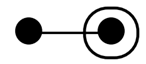 as a component, which is not a legal simple Weyl diagram). Hence we have to encircle node \(1\). Then we must see in the residue of node \(1\) a Weyl diagram of type \(\mathsf{D}_{n-1}\). But since we encircled node \(1\), we either have to encircle node \(3\), or none of nodes \(2,3,4,5\) are encircled while node \(6\) is. The former leads to \(n-1\) being even and to \(\mathsf{D}_{n-1;\frac{n-1}{2}}^2\) in the residue, hence to \(\mathsf{E_{7;4}}\); the latter leads to \(\mathsf{E}_{n;n-4}\).
The remaining cases \(\mathsf{F_4}\) and \(\mathsf{I}_{n}\) are easy.
Now consider a Weyl diagram of class 2. If no orbit of length \(2\) is encircled, then we can only have type \(\mathsf{D}_n\), and this leads to \(\mathsf{D}_{n,i}^1\). If one orbit of length \(2\) is encircled, then all of them are (since there is no simple Weyl diagram of class 2 with uncircled nodes), and all of their neighbours are, and this leads to \(\mathsf{^2A}_{2n+1,n+1}^1\), \(\mathsf{D}_{n,n-1}^1\), \(\mathsf{^2E_{6;4}}\), \(\mathsf{^2F_{4;2}}\) and \(\mathsf{^2I_{2,1}}(2m)\).
This concludes the proof of Main Result 1.4. We will now use this to prove Main Result 1.1. Ovoidal subcomplexes are of class \(1\) if their Weyl diagrams are of class \(1\); otherwise they are said to be of class \(2\).
Proofs of main Results 1.1 and 1.2
We go type by type, clearly indicating under which conditions, weaker than stated in Main Result 1.1, the latter result holds. We also provide the necessary definitions to understand the Weyl substructures. We then discuss the elementwise stabiliser of the Weyl substructure to prove Main Result 1.1. All of this will be done in the appropriate Lie incidence geometry.
Projective spaces: type \(\mathsf{A}_n\)
Buildings of type \(\mathsf{A}_n\) will be approached via their \(1\)-Grassmannian, a geometry of type \(\mathsf{A}_{n,1}\), which is simply a projective space of dimension \(n\), usually denoted \(\mathsf{PG}(n,\mathbb{K})\), if the ground division ring is \(\mathbb{K}\) (see Subsection 2.1).
We begin with Weyl substructures of class \(1\). A line spread \(\mathcal{S}\) of \(\mathsf{PG}(n,K)\) is a partition of the point set into lines. A line spread \(\mathcal{S}\) is a composition spread if it induces a line spread in every subspace generated by an arbitrary number of members of \(\mathcal{S}\). Line spreads that are elementwise fixed under a collineation of \(\mathsf{PG}(n,\mathbb{K})\) are automatically composition. If \(\mathsf{PG}(n,\mathbb{K})\) admits a composition line spread, then it is easy to see that \(n\) has to be odd (indeed, letting \(n\) be the smallest counter example, we may suppose that there is a subspace \(U\) of dimension \(n-1\) in which \(\mathcal{S}\) induces a line spread. Then the line of \(\mathcal{S}\) through a point outside \(U\) intersects \(U\), a contradiction).
A line spread of \(\mathsf{PG}(3,\mathbb{K})\) is called a bi-spread if every plane of \(\mathsf{PG}(3,\mathbb{K})\) contains a line of the spread.
Proposition 4.1. A subcomplex \(\Sigma\) of \(\mathsf{PG}(n,\mathbb{K})\) is ovoidal of class \(1\) if, and only if, it corresponds to all subspaces generated by the elements of a composition line spread of \(\mathsf{PG}(n,\mathbb{K})\) (and \(n\) is necessarily odd), with the additional property that every spread induced in the subspace spanned by two members of the spread, is a bi-spread.
Proof. We proceed by induction on \(n\), the result for \(n=3\) following directly from the definition of ovoid of a polar space of type \(\mathsf{D_3}\) (remember the Weyl diagram of \(\Sigma\) is \(\mathsf{A_{3;1}^2}=\mathsf{D_{3;1}^1}\) in this case).
Let \(n>3\). First suppose \(\Sigma\) is ovoidal of type 1. Then the Weyl diagram of \(\Sigma\) is \(\mathsf{A}_{2m+1;n}^2\), \(n=2m+1\). Let \(L\in \Sigma\) be a line of \(\mathsf{PG}(n,\mathbb{K})\). The induction hypothesis implies that each plane \(\pi\) containing \(L\) is contained in a unique subspace \(S\) of dimension \(3\) belonging to \(\Sigma\). Considering the residue of \(S\) we see that \(\pi\) does not contain any member of \(\Sigma\) except for \(L\), and that every point of \(\pi\) is contained in some line belonging to \(\Sigma\). This shows that the line set of \(\Sigma\) is a line spread of \(\mathsf{PG}(n,\mathbb{K})\).
Consider an arbitrary number of lines of \(\Sigma\). We may assume \(L\) is amongst these. Then, by induction, the subspaces of dimension \(3\) of \(\Sigma\) through \(L\) induce a spread in the residue at \(L\) of the subspace \(U\) generated by all these lines. Since the lines of \(\Sigma\) induce spreads in each of these subspaces of dimension \(3\), we see that the lines of \(\Sigma\) induce a spread in \(U\). Hence the lines of \(\Sigma\) define a composition line spread (with the mentioned additional property) and induction implies that the subspace generated by an arbitrary number of lines of \(\Sigma\) belongs to \(\Sigma\). Clearly, by taking residues, every member of \(\Sigma\) is generated by lines of \(\Sigma\), which completes the proof of the “only if” direction of the proposition.
Next assume that \(\Sigma\) is a composition line spread satisfying the mentioned additional property. First assume \(n=5\). We have to show that the solids (which is short for \(3\)-dimensional subspaces) of \(\Sigma\) through a given line \(L\in\Sigma\) form a bi-spread in the residue of \(L\). Let \(\pi\) be any plane through \(L\) and pick \(x\in\pi\setminus L\). Since \(\Sigma\) is a line spread, there is a line \(M\in\Sigma\) containing \(x\). Since \(\Sigma\) is a composition spread, the solid generated by \(L\) and \(M\) belongs to \(\Sigma\) and clearly contains \(\pi\). Now let \(U\) be a \(4\)-dimensional subspace of \(\mathsf{PG}(n,\mathbb{K})\) containing \(L\). Select two distinct solids \(S_1,S_2\in\Sigma\) containing \(L\). Next, select lines \(L_1\subseteq S_1\) and \(L_2\subseteq S_2\) distinct from \(L\). The property of \(\Sigma\) being a composition line spread implies that the solid \(S\) generated by \(L_1,L_2\) belongs to \(\Sigma\) and is disjoint from \(L\). Hence \(U\cap S\) is a plane, and since the set of lines of \(\Sigma\) in \(S\) defines a bi-spread of lines, the plane \(U\cap S\) contains a member \(N\) of it. Hence \(U\) contains the solid of \(\Sigma\) generated by \(L\) and \(N\). So \(\Sigma\) is an ovoidal subcomplex of class I.
Now assume \(n\geq 7\). We have to show that, given a \((2i-1)\)-dimensional subspace \(U\) belonging to \(\Sigma\), and a \((2i+3)\)-dimensional subspace \(W\in\Sigma\) containing \(U\), \(2i+3\leq n\), the members of dimension \(2i+1\) of \(\Sigma\) containing \(U\) and contained in \(W\) form a bi-spread of the residue of \(U\) in \(W\). If \(2i+3\leq n-2\), then this follows from the induction hypothesis, so assume \(2i+3=n\), that is, \(W\) is the whole space. Select a line \(L\in\Sigma\) in \(U\). Then in the residue of \(L\), the members of \(\Sigma\) define a composition line spread satisfying the additional property thanks to the case \(n=5\) above. The induction hypothesis now implies the assertion. \(\square\)
Now Main Result 1.5(iii) follows immediately from [37, Theorem 1]. Note that, over a non-commutative division ring, one does not know whether the simple spread induced in a \(3\)-space spanned by two lines of a given composition spread is a bi-spread! However, in view of Theorem 4.5 below, if a non-trivial collineation fixes a line spread of a \(3\)-dimensional projective space elementwise, then the line spread is a bi-spread. Hence we might revise the definition of Weyl substructure of class \(1\) in projective spaces so as to include that (geometric) property. This way, Weyl substructures in buildings of type \(\mathsf{A}_n\) will be completely equivalent to ovoidal subcomplexes. Now, this might make one wonder whether the rigid examples from [37] are really bi-spreads. If not, then they would not be counterexamples. But they are, and we will show now. We also show that in the rank 1 case, such a spread is not elementwise fixed under a duality. Clearly, the only possible dualities that can elementwise fix a spread are null polarities as each point lies on a spread line and would hence be isotropic. Note that null polarities, also called symplectic polarities, are the type-interchanging involutory automorphisms associated to non-singular alternating bilinear forms of the underlying vector space.
Lemma 4.2. Let \(\mathcal{S}\) be a composition line spread of some projective space of dimension at least \(5\) defined over a commutative field. Let \(S\) be a solid in which \(\mathcal{S}\) induces a simple line spread \(\mathcal{S}_S\). Then \(\mathcal{S}_S\) is a bi-spread. If \(\mathcal{S}\) is rigid, then \(\mathcal{S}_S\) is not a symplectic spread, that is, it is not elementwise fixed under any symplectic polarity of \(S\).
Proof. All spreads \(\mathcal{S}_S\) are classified in [37, Theorem 1]. There are four classes of examples, two of which are not rigid (the regular spread and the spread emerging from Galois descent). Let us handle only one of the two classes of rigid spreads; the other can be dealt with in a similar fashion.
We use the notation of [37]. Let \(\mathbb{F}\) be a field with \(\mathop{\mathrm{\mathsf{char}}}\mathbb{F}=2\), let \(\mathbb{F}’\) be a subfield of \(\mathbb{F}\) and \(t\in\mathbb{F}\setminus\mathbb{F}’\) such that \(t^2\in\mathbb{F}’\) and assume that \(\mathbb{F}\) is \(2\)-dimensional over \(\mathbb{F}’\), that is, every element \(x\) of \(\mathbb{F}\) can be written as \(x=x_1+x_2t\), with \(x_1,x_2\in\mathbb{F}’\). Let \(F,G\in{\mathbb{F}’}^\times\) be such that the quadratic polynomial \(x^2+Gx+F\) is irreducible over \(\mathbb{F}’\). For each \(a=a_1+a_2t\) and \(b=b_1+b_2t\), \(a,i,b_i\in\mathbb{F}’\), \(i=1,2\), we define the points \(p(a,b)\) and \(q(a,b)\) in standard coordinates as \[p(a,b)=(a,b,1,0)\mbox{ and }q(a,b)=(Ga_2t+Fb,a+Gb_1,0,1).\]
Then \(\mathcal{S}_S=\{\left\langle p(a,b),q(a,b)\right\rangle\mid a,b\in \mathbb{F}\}\cup\{\left\langle (1,0,0,0),(0,1,0,0)\right\rangle\}\), where for clarity, the line generated by two points \(x,y\) is denoted as \(\left\langle x,y\right\rangle\). Now let \(L(a,b)\in\mathcal{S}_S\) denote the line generated by \(p(a,b)\) and \(q(a,b)\), and set \(L(\infty)=\left\langle 1,0,0,0),(0,1,0,0)\right\rangle\). One easily calculates that a set of equations for \(L(a,b)\) is given by (ordering the coordinates as \((X_1,X_2,X_3,X_4)\)) \[\begin{cases} X_1+aX_3+(Ga_2t+Fb)X_4=0,\\
X_2+bX_3+(a+Gb_1)X_4=0.
\end{cases}\]
Hence in the dual projective space, a generic spread line is given in (dual) coordinates by \[\left\langle (1,0,a,Fb+Ga_2t),(0,1,b,a+Gb_1)\right\rangle.\]
Rearranging the order of the coordinates (writing them in opposite order), and replacing \(a_1\) with \(a1+Gb_1\), we obtain the projectively equivalent form \[\left\langle (a,b,1,0), (Fb+Ga_2t,a+Gb_1,0,1)\right\rangle,\] which is exactly a generic member of \(\mathcal{S}_S\) above. Hence \(\mathcal{S}_S\) is self-dual and consequently, it is a bi-spread.
Now suppose for a contradiction that \(\mathcal{S}_S\) is a symplectic spread. A symplectic form is given by \[\sum_{1\leq i<j\leq 4}\lambda_{ij}(X_iY_j+X_jY_i), \ \ \ \lambda_{ij}\in\mathbb{F}.\]
Expressing that \((1,0,0,0)\) and \((0,1,0,0)\) are perpendicular, and similarly for \((0,0,1,0)\) and \((0,0,0,1)\), we deduce \(\lambda_{12}=\lambda_{34}=0\). Now \(p(a,b)\) is perpendicular to \(q(a,b)\) if, and only if, \[\lambda{14}a+\lambda_{24}b+\lambda_{13}(Ga_2t+Fb)+\lambda_{23}(a+Gb_1)=0.\]
Since this must hold for every \(a_1,a_2,b_1,b_2\in\mathbb{F}’\), we easily deduce \[\begin{cases}\lambda_{14}+\lambda_{23}=0,\\
\lambda_{14}+G\lambda_{13}+\lambda_{23}=0,\\
\lambda_{24}+F\lambda_{13}+G\lambda_{23}=0,\\
\lambda_{24}+F\lambda_{13}=0.
\end{cases}\]
We now see \(\lambda_{13}=\lambda_{14}=\lambda_{23}=\lambda_{24}=0\), a contradiction, which proves the lemma. \(\square\)
We now consider Weyl substructures of class \(2\). These will be related to symplectic polarities as defined above. The totally isotropic subspaces (with respect to the alternating form of the symplectic polarity) are the singular subspaces of a polar space, called a symplectic polar space. The points of the polar space are al points of \(\mathsf{PG}(n,\mathbb{K})\) and \(n\) is necessarily odd. By [31, § 8.3.2], a symplectic polarity in \(\mathsf{PG}(n,\mathbb{K})\) is equivalent to a symmetric reflexive relation on the point set of \(\mathsf{PG}(n,\mathbb{K})\) such that the points in relation with a given point form a hyperplane (and then this hyperplane is the image of the given point under the action of the polarity).
The next proposition not only contributes to Main Result 1.1, but also shows Main Result 1.5(ii) for absolute type \(\mathsf{A}_n\).
Proposition 4.3. A subcomplex \(\Sigma\) of \(\mathsf{PG}(n,\mathbb{K})\) is ovoidal of class \(2\) if, and only if, it corresponds to all totally singular subspaces of a non-degenerate alternating form, or, equivalently, to all absolute subspaces of a symplectic polarity \(\theta\). More precisely, the members of \(\Sigma\) are the flags of size \(2\) fixed under the polarity.
Proof. Let first \(\Sigma\) be the complex of all totally singular subspaces of a non-degenerate alternating form in \(\mathsf{PG}(2m+1,\mathbb{K})\). Let \(U\subseteq W\) be two totally singular subspace with \(2+\mathop{\mathrm{\mathsf{dim}}}U=\mathop{\mathrm{\mathsf{dim}}}W\leq m\). Let \(U^\theta\) and \(W^\theta\) be their respective images under the corresponding symplectic polarity. Then we have to show that the set of totally isotropic subspaces \(V\) with \(U\subseteq V\subseteq W\) and \(\mathop{\mathrm{\mathsf{dim}}}V=1+\mathop{\mathrm{\mathsf{dim}}}U\), together with the images \(V^\theta\), forms a simple ovoidal subcomplex. This defines indeed an ovoid-spread pairing of the corresponding generalized digon as every subspace \(V\) with \(U\subseteq V\subseteq W\) and \(\mathop{\mathrm{\mathsf{dim}}}V=1+\mathop{\mathrm{\mathsf{dim}}}U\) is totally isotropic. Likewise, if \(U\) is totally isotropic with \(\mathop{\mathrm{\mathsf{dim}}}U=m-1\), then every subspace \(V\) with \(U\leq V\leq U^\theta\) and \(\mathop{\mathrm{\mathsf{dim}}}V=m\) is totally isotropic and hence defines a simple ovoidal subcomplex of the corresponding residue.
Conversely, let \(\Sigma\) be an ovoidal subcomplex with Weyl diagram \(\mathsf{^2A}_{2m+1;m+1}\). We use induction on \(n\) to prove the assertion. We first claim that every point \(x\) of \(\mathsf{PG}(2m+1,\mathbb{K})\) is contained in a (point-hyperplane) flag of \(\Sigma\). We know that there is at least one point-hyperplane pair \((p,H)\) in \(\Sigma\). Induction implies that every line \(L\) through \(p\) in \(H\) is contained in a line-subhyperplane pair \((L,S)\) of \(\Sigma\) (and we fix such an \(L\)). By the definition of ovoidal subcomplex, every hyperplane \(G\) through \(S\) (in particular one that contains \(x\)) is contained in a unique point-hyperplane pair \((q,G)\) belonging to \(\Sigma\). Replacing \((p,H)\) by\((q,G)\) if necessary, this means that we can assume that \(x\in H\), and we may also assume that \(px=L\). As before, induction implies that \(x\) is contained in a unique point-hyperplane pair \((x,X)\) with \(S\subseteq X\) and \(X\neq H\). This not only proves our claim, but it also shows that, given \(H\), the point \(p\) is unique with \((p,H)\in\Sigma\) (as we may assume for a contradiction that also \((x,H)\in\Sigma\), and this leads, by the above argument, indeed to the contradiction \(X=H\)).
Now noting that in the previous argument \(p\in X\), we see that the relation \(p\sim q\) if \(q\) is contained in the unique hyperplane \(H\) such that \((p,H)\in\Sigma\) is symmetric and reflexive, and has the property that the set of points in relation to a given point is precisely a hyperplane. Hence we obtain a symplectic polarity, and using induction it is now routine to check that \(\Sigma\) consists precisely of the fixed flags of size \(2\). \(\square\)
Now, the following is Theorem 4.2 of [17].
Proposition 4.4 (Theorem 4.2 of [17]). A non-trivial automorphism \(\theta\) of a projective space is uniclass if, and only if, it is either an anisotropic duality, or a symplectic polarity, or it fixes a composition line spread elementwise.
The proof of this proposition also showed that a non-trivial collineation elementwise fixing a line spread does not fix any point. Putting this together with Propositions 4.1, 4.3 and 4.4, we obtain the following result.
Theorem 4.5. An automorphism \(\theta\) of a building of type \(\mathsf{A}_n\) is uniclass if, and only if, it is either an anisotropic duality, or it pointwise fixes an ovoidal subcomplex.
Proof. Suppose first that \(\theta\) is non-trivial and pointwise fixes an ovoidal subcomplex \(\Sigma\). If \(\Sigma\) is of class 1, then this follows from Proposition 4.4. If \(\Sigma\) is of class 2, then it must be a duality since every point belongs to a member of \(\Sigma\) and hence would be fixed, leading to the identity. But then \(\theta\) must coincide with the polarity \(\rho\) associated to \(\Sigma\) by Proposition 4.3, because \(\theta\rho\) is type preserving and fixes \(\Sigma\) pointwise, and we just argued that only the identity can do this.
Next suppose that \(\theta\) is uniclass. If \(\theta\) is a duality, then Proposition 4.4 implies it is a symplectic polarity, and Proposition 4.3 shows that it pointwise fixes an ovoidal subcomplex of type 2. If \(\theta\) is non-trivial and type preserving, then by Proposition 4.4, it elementwise fixes a composition line spread \(\mathcal{S}\). In view of Proposition 4.1, it suffices to show that the spread induced by two members \(L_1,L_2\in\mathcal{S}\) in \(\left\langle L_1,L_2\right\rangle\), is a bi-spread. Let \(\pi\) be any plane i \(\left\langle L_1,L_2\right\rangle\). Pick \(x\in \pi\cap\pi^\theta\) and note that, by the comment following Proposition 4.4, \(x\neq x^\theta\). Since \(\left\langle x,x^\theta\right\rangle\) is fixed, \(x^\theta\) also belongs to \(\pi\cap\pi^\theta\), and so the \(\left\langle x,x^\theta\right\rangle\subseteq\pi\) with obviously \(\left\langle x,x^\theta\right\rangle\in\mathcal{S}\).
Remember that we obtain the identity by considering the Weyl structure consisting of the whole building. The corresponding Weyl diagram is full. \(\square\)
Generalized polygons: type \(\mathsf{I}_2^{(d)}\)
Generalized polygons are the point-line geometries associated to spherical buildings of rank 2. More exactly, a generalized \(d\)-gon \(\Gamma\), \(d\geq 2\), is a point-line geometry for which the incidence graph has diameter \(d\) and girth \(2d\). As we are only concerned with thick buildings, we also assume that each vertex has valency at least \(3\). In generalized polygons \(\Gamma\) it is customary to call chambers just (point-line) flags. We measure the distance between points and lines in the incidence graph and denote that distance function as \(\delta_\Gamma\).
Recall that an ovoid or spread (also called distance-\(d/2\) ovoid or distance-\(d/2\) spread, respectively, in [35]) of a generalized \(d\)-gon, with \(d\) even, is a set of mutually opposite points or lines, respectively, such that every point and line is at distance at most \(d/2\) from at least one member of the ovoid or spread, respectively. An ovoid-spread pairing is a set of flags such that the points of the flags form an ovoid, and the lines of the flags form a spread. Clearly, ovoids and spreads do not exist if \(d\) is odd. Therefore we consider below only generalized \(2d\)-gons.
Since in generalized polygons only simple ovoidal subcomplexes exist, and by definition these are the same as Weyl substructures, there is nothing to prove concerning Main Result 1.1. Concerning Main Result 1.1, we have to show that only the identity or a polarity can pointwise fix an ovoid-spread pairing. We begin with dualities.
Proposition 4.6. A duality \(\theta\) of a generalized \(2d\)-gon \(\Gamma\) elementwise fixes an ovoid-spread pairing if, and only if, it is a polarity.
Proof. From Proposition 7.2.5 and Definitions 7.2.6 of [35], we deduce that the fix structure of a polarity is always an ovoid-spread pairing.
Now let \(\theta\) be a duality of \(\Gamma\) elementwise fixing an ovoid-spread pairing \((\mathcal{O},\mathcal{S})\). Let \(p\) be any point. Then by the definitions of ovoid and spread, \(p\) is at distance at most \(d\) from at least one member of \(\mathcal{O}\cup\mathcal{S}\), and we can make the corresponding shortest path longer so that, without loss of generality, we may assume that there is a unique flag \(\{x,L\}\), with \(x\in\mathcal{O}\) and \(L\in\mathcal{S}\) such that \(p\) has distance \(d-1\) to one of \(x\) or \(L\), and distance \(d\) to the other. Let us, to fix the ideas, assume that \(\delta_\Gamma(p,L)=d=\delta_\Gamma(p,x)+1\) (then \(d\) is odd; the case \(d\) even is handled similarly). Consider an arbitrary line \(M\) through \(p\) distinct from the one at distance \(d-1\) from \(L\). Then there is a unique flag \(\{x’,L’\}\), with \(x’\in\mathcal{O}\) and \(L’\in\mathcal{S}\) with \(\delta_\Gamma(M,L’)=d-1\) and \(\delta_\Gamma(M,x’)=d\). It follows that \(\theta\) interchanges the unique shortest path connecting \(x\) and \(L’\) with the unique shortest path connecting \(L\) and \(x’\). In particular \(\theta\) acts as an involution on the union of these paths, hence \(p^{\theta^2}=p\). The proposition follows. \(\square\)
Now we handle the case of a collineation. This is a consequence of the following more general result.
Proposition 4.7. A collineation \(\theta\) of a generalized \(2d\)-gon \(\Gamma\) elementwise fixing an ovoid \(\mathcal{O}\) does not fix any other point or line, unless it is the identity.
Proof. The statement is trivial for \(d=1\), so we assume \(d\geq 2\).
Suppose that \(\theta\) fixes some point or line, say \(x\), not belonging to the ovoid. Let \(i\) be the minimal distance from \(x\) to some element of \(\mathcal{O}\), say \(\delta_\Gamma(x,p_x)=i\), \(p_x\in\mathcal{O}\). By the definition of ovoid, \(i\leq d\). We claim that \(\theta\) fixes each element \(y\) incident with \(x\). If \(i=d\), then, by parity, \(y\) is at distance \(d-1\) from some member \(p_y\in\mathcal{O}\). By minimality of \(i\), we have \(\delta_\Gamma(p_y,x)=i=d\), implying that the path of length \(d\) joining \(p_y\) with \(x\), which contains \(y\), is unique; hence \(y\) is fixed. Now assume \(1\leq i<d\). If \(\delta_\Gamma(p_x,y)=i-1\), then \(y\) is fixed by uniqueness of such a point with the given distances. Suppose now \(\delta_\Gamma(p_x,y)=i+1\). We select an element \(z\) at distance \(d-i\) from \(y\) and distance \(d+1\) from \(p_x\); then \(\delta_\Gamma(z,x)=d+1-i\). Also, again by parity, \(z\) is at distance at most \(d-1\) from some point \(p_z\in\mathcal{O}\). Then \(\delta_\Gamma(p_z,x)\leq (d-1)+(d+1-i)=2d-i<2d\). This implies that every line or point on a minimal path from \(p_z\) to \(x\) is fixed. In particular \(y\) is fixed and the claim is proved.
We can now interchange the roles of \(x\) and an arbitrary element incident with \(x\). Then all elements at distance \(2\) from \(x\) are fixed. Going on like this, all points and lines are fixed by connectivity, and \(\theta\) is the identity. \(\square\)
We now immediately deduce the following result.
Theorem 4.8. An automorphism \(\theta\) of a building of type \(\mathsf{I}_2(d)\) is uniclass if, and only if, it is either anisotropic or it pointwise fixes an ovoidal subcomplex.
Regarding Main Result 1.5, there is nothing to prove here.
Polar spaces: types \(\mathsf{B}_n\) and \(\mathsf{D}_n\)
Let \(\Gamma\) be a polar space of rank \(n\geq 2\) and let \(U\) be a singular subspace of dimension \(i\leq n-2\). As explained in Subsection 2.1, we denote by \(\mathop{\mathrm{\mathsf{Res}}}_\Gamma(U)\) the polar space obtained from \(\Gamma\) and \(U\) by taking as point set the set of singular subspaces of dimension \(i+1\). The lines, if they exist, are then determined by the singular subspaces of dimension \(i+2\) containing \(U\).
Let \(\Gamma\) be a polar space. An ovoid is a set of points intersecting every maximal singular subspace in exactly one point. A subspace of \(\Gamma\) is called ideal if it induces an ovoid in the residue of each hyperplane of each of its maximal subspaces. A subspace is said to have corank \(i\) if each singular subspace of dimension \(i\) intersects the subspace non-trivially and if there exists a singular subspace of dimension \(i-1\) disjoint from it. Not all subspaces admit a corank. Ideal subspaces of corank \(i\) are themselves polar spaces of rank \(n-i\) by [17, Lemma 4.3]. Recall the following proposition proved in [17].
Proposition 4.9 (Proposition 4.4 in [17]). Let \(\theta\) be an automorphism of a polar space \(\Gamma\) of rank \(r\) admitting at least one fixed point. Then it is uniclass if, and only if, the fixed points form an ideal subspace.
It follows immediately from the very definition that an ideal subspace of corank \(i\) is a convex ovoidal subcomplex (convex since it is a polar space on its own, where the collinearity relations correspond, hence a subbuilding). We now show the converse.. We first treat a special case where the condition (WCC) is not needed. We start by proving a lemma applicable to all cases.
Lemma 4.10. An ovoidal subcomplex \(\Sigma\) of type \(\mathsf{B}_{n;n-i}^1\), or \(\mathsf{D}_{n;n-i}^1\) of the polar space \(\Gamma\) contains at least one member of \(\Sigma\) of dimension \(n-i-1\) in each maximal singular subspace \(M\), and it contains such a member through each point of \(\Sigma\) in \(M\).
Proof. We show this by induction on \(n-i\geq 1\). For \(n-i=1\), this is by definition the case, since \(\Sigma\) is then just a simple ovoidal subcomplex, hence an ovoid. Now assume \(n-i\geq 2\). Let \(M\) be a maximal singular subspace of \(\Gamma\) and pick a point \(p\in\Sigma\). If \(p\in M\), then looking in the residue at \(p\), the elements of \(\Sigma\) containing \(p\) form an ovoidal subcomplex of the residue, and hence the induction hypothesis yields a subspace of dimension \(n-i-1\) in \(M\). If \(p\notin M\), then there is a unique maximal singular subspace \(M’\) containing \(p\) and intersecting \(M\) in a subspace \(H\) of dimension \(n-2\). The previous argument yields a subspace of dimension \(n-i-1\geq 1\) through \(p\) in \(M’\), which necessarily intersects \(H\), and hence \(M\), in at least a point \(p’\). With \(p’\) in the role of \(p\), the previous argument now concludes the proof. \(\square\)
Proposition 4.12. The union \(U(\Sigma)\) of all members of an ovoidal subcomplex \(\Sigma\) of type \(\mathsf{B}_{n;n-1}^1\) or \(\mathsf{D}_{n;n-1}^1\) in a polar space of type \(\mathsf{B}_n\) or \(\mathsf{D}_n\), respectively, with \(n\geq 3\) is an ideal subspace of corank \(1\).
Proof. We first claim that \(U(\Sigma)\) is a subspace. Let \(x_1,x_2\in U(\Sigma)\) be two collinear points. Select a maximal singular subspace \(M\) containing \(x_1\) and \(x_2\). Lemma 4.10 yields singular subspaces \(U_i\ni x_i\) of dimension \(n-2\) contained in \(M\) and belonging to \(\Sigma\). A dimension argument implies that these have a subspace \(U\) of dimension \(n-3\geq 0\) in common. The definition of ovoidal subcomplex requires that \(U_1=U_2\); hence \(x_1\) and \(x_2\) are contained in a common higher dimensional member of \(\Sigma\), showing the claim.
Now by definition of ovoidal subcomplex, \(U(\Sigma)\) is ideal, and it is of corank \(1\) by Lemma 4.10. \(\square\)
Proposition 4.13. If the ovoidal subcomplex \(\Sigma\) of type \(\mathsf{B}_{n;n-i}^1\) or \(\mathsf{D}_{n;n-i}^1\), \(i\geq 1\), of a polar space \(\Gamma\) satisfies condition (WCC), or, slightly weaker, does not contain two of its maximal singular subspaces in the same maximal singular subspace of \(\Gamma\), then its union \(U(\Sigma)\) is an ideal subspace of corank \(i\).
Proof. If \(U(\Sigma)\) is a subspace, then the definition of ovoidal subcomplex implies that \(U(\Sigma)\) is ideal, and it is of corank \(i\) by Lemma 4.10.
Let the Weyl diagram of \(\Sigma\) be \(\mathsf{B}_{n;n-i}^1\) or \(\mathsf{D}_{n;n-i}^1\). If \(U(\Sigma)\) is not a subspace, then arguing as in the first paragraph of the proof of Proposition 4.12, we obtain two distinct singular subspaces \(U_1\) and \(U_2\) of dimension \(n-i-1\) in a maximal singular subspace \(M\). The fact that the span of \(U_1\) and \(U_2\) is contained in the convex closure of \(\Sigma\) contradicts now condition (WCC) and the weaker condition mentioned in the proposition. \(\square\)
We now show Main Result 1.5(v), hence for ideal subspaces of corank at most \(n-1\) in polar spaces of rank \(n\), and also Main Result 1.5(i) for Weyl diagram \(\mathsf{D}_{n;i}^1\), \(2\leq i\leq n-1\), \(n\geq 4\). First a lemma.
Lemma 4.14. Let \(\mathsf{PG}(V)\) be the projective space naturally associated to the (right) vector space \(V\) over some skew field \(\mathbb{K}\). Let \(W\) and \(U\) be subspaces such that \(\mathop{\mathrm{\mathsf{dim}}}U=\mathop{\mathrm{\mathsf{codim}}}W=d\in\mathbb{N}\) and \(\mathop{\mathrm{\mathsf{dim}}}W\geq d\). Let \(A\) and \(B\) be two subspaces of \(V\), both complementary to \(W\) and such that \(U\subseteq \left\langle A,B\right\rangle\) with \(U\) disjoint from both \(A\) and \(B\). Suppose that \(W\cap U\), \(\left\langle W,U\right\rangle\cap A\) and \(\left\langle W,U\right\rangle\cap B\) do not contain respective vectors that are linearly dependent. Then there exists a linear map fixing \(W\) pointwise, stabilising all subspaces containing \(U\), and mapping \(A\) to \(B\).
Proof. We may restrict the vector space \(V\) to \(\left\langle A,B\right\rangle\), and afterwords extend the linear map over \(W\) with the identity on a complementary subspace. Hence we replace \(W\) with \(W\cap\left\langle A,B\right\rangle\).
Set \(\ell=\mathop{\mathrm{\mathsf{dim}}}W\cap U\). Let \(\{e_j\mid 1\leq j\leq\ell\}\) be a basis for \(W\cap U\), and extend this to a basis \(\{e_j\mid 1\leq j\leq d\}\) of \(W\). For each \(j \in\{1,2,\ldots,\ell\}\), there exist unique \(a_j\in A\) and \(b_j\in B\) such that \(e_j=a_j+b_j\) (by complementarity of \(A\) and \(B\) in \(\left\langle A,B\right\rangle\supseteq U\)). Similarly, there exist \(u_j,u’_j\in U\) such that \(e_j=u_j+a_j=u’_j+b_j\), \(\ell+1\leq j\leq d\). We claim that \(\{a_j\mid 1\leq j\leq d\}\) is a basis for \(A\). Indeed, the projection of \(\left\langle e_{\ell+1},\ldots,e_d\right\rangle\) from \(U\) onto \(A\) is a subspace of \(A\) of dimension \(d-\ell\), which coincides precisely with \(\left\langle W,U\right\rangle\cap A\). Also, clearly, since \(A_\ell=:\left\langle a_j\mid 1\leq j\leq \ell\right\rangle\) is the projection of \(W\cap U\) onto \(A\) from \(B\), we deduce that \(\mathop{\mathrm{\mathsf{dim}}}A_\ell=\ell\). If some vector of \(A_\ell\), say \(k_1a_1+\cdots + k_\ell a_\ell\) would belong to \(\left\langle W,U\right\rangle\), then the vectors \(k_1e_1+\cdots k_\ell e_\ell\), \(k_1a_1+\cdots + k_\ell a_\ell\) and \(k_1b_1+\cdots + k_\ell b_\ell\) are linearly dependent vectors in \(\left\langle W,U\right\rangle\), contrary to our assumptions. The claim now follows. Likewise, \(\{b_j\mid 1\leq j\leq d\}\) is a basis for \(B\). Hence, by the complementarity of \(W\) and both \(A\) and \(B\), The sets \(\{a_j,e_j \mid 1\leq j\leq d\}\) and \(\{b_j,e_j \mid 1\leq j\leq d\}\) are bases for \(V\). Then the linear map defined on the basis by \(e_j\mapsto e_j\) and \(a_j\mapsto b_j\), for all \(j\in\{1,2,\ldots,d\}\), fixes \(W\) pointwise and maps \(A\) to \(B\). From our definitions also follows that \(u_j\) is mapped onto \(u’_j\), for all \(j\in\{\ell+1,\ldots,d\}\), hence \(U\) is stabilised. It also easily follows from the definitions of the base vectors that \(\left\langle U,a_j\right\rangle=\left\langle U,b_j\right\rangle\), for \(1\leq j\leq d\). Hence all subspaces containing \(U\) are stabilised and the lemma is proved. \(\square\)
We say that the map in the previous lemma has axis \(W\) and centre \(U\).
Proposition 4.15. An ideal subspace of corank \(i\) at most \(n-2\) of a polar space \(\Gamma\) of rank \(n\) is always the fix structure of a non-trivial collineation, except possibly when \(\Gamma\) is embeddable in projective spaces of different dimensions. In particular, ovoidal subcomplexes with Weyl diagram \(\mathsf{D}_{n;i}^1\), \(2\leq i\leq n-1\), \(n\geq 4\), are never rigid.
Proof. By [23] and [24, Main Result 1], there do not exist ideal subspaces of corank 1 in non-embeddable polar spaces. Hence we may assume that \(\Gamma\) is embeddable, say in the projective space \(\Pi\). Let \(X\) be the point set of \(\Gamma\) and \(Y\) the ideal subspace of corank \(i\) at most \(n-2\). Then our assumption and the main result of [4] yield a subspace \(S\) of \(\Pi\) such that \(S\cap X=Y\). Let \(T=S^\rho\), with \(\rho\) the underlying polarity, which is non-degenerate by uniqueness of the embedding. We claim that \(T\cap X=\varnothing\). Indeed, suppose for a contradiction that \(x\in T\cap X\). Then \(x\in T\setminus S\) as \(Y\) is non-degenerate. Pick a singular subspace \(A\) of \(Y\) of dimension \(n-i-2\). Then \(\mathop{\mathrm{\mathsf{Res}}}_Y(A)\) is an ovoid in \(\mathop{\mathrm{\mathsf{Res}}}_\Gamma(A)\), each point of which is collinear to the point corresponding to \(x\). This contradicts [15, Lemma 3.1.3]. Note that this argument in fact shows that no point of \(\Gamma\) is collinear to all points of \(Y\).
Let \(U\) be a singular subspace of \(\Gamma\) complementary to \(S\) (that is, of dimension \(i-1\)), which exists by the definition of subspace of corank \(i\). Set \(\Pi’=\left\langle T,U\right\rangle\). Then \(\Pi’\) intersects \(X\) in the point set \(X’\) of an induced polar space \(\Gamma’\) of rank at least \(i\) (because it contains \(U\)) and at most \(i\) (since \(T\) does not contain points of \(X\)), hence rank exactly \(i\) (note for the moment we do not know whether \(\Gamma’\) is non-degenerate, that is, whether it contains no point collinear to all others; we will prove this below). We claim that \(X’\cap S=\varnothing\). Indeed, suppose for a contradiction that \(x’\in X’\cap S\). Then \({x’}^{\perp}\) contains a singular subspace of \(\Pi’\) of dimension \(i-1\), necessarily disjoint from \(T\) (as \(T\cap X=\varnothing\)), and \({x’}^\perp\) also contains \(T\), as \(T=S^\rho\) and \(x’\in S\). Hence \({x’}^\rho\) contains \(\Pi’\), and so \(\left\langle x’,U\right\rangle\) is singular. But since \(\mathop{\mathrm{\mathsf{dim}}}\left\langle x’,U\right\rangle=i\), it intersects \(T\) in a point, a contradiction as \(T\cap X=\varnothing\). We can now also prove that \(\Gamma’\) is non-degenerate. Indeed, any point \(x’\) collinear to all points satisfies \(T\subseteq\Pi’\subseteq {x’}^\rho\), which implies \(x\in S\), contradicting the previous claim.
Hence \(\Gamma’\) is a true non-degenerate polar space and we can pick a maximal singular subspace \(U’\) of it disjoint from \(U\). Set \(U_0=\left\langle S,T\right\rangle\cap U\) and \(U_0’=\left\langle S,T\right\rangle\cap U’\). We claim dat \(\left\langle U_0,U_0’\right\rangle\) is disjoint from \(S\cap T\). This is equivalent with \(\left\langle S\cap T,U_0,U_0’\right\rangle=\left\langle S,T\right\rangle\). This, in turn, is equivalent to \[(S\cap T)^\rho\cap U_0^\perp\cap U_{0′}^\perp=\varnothing.\]
Set \(\mathop{\mathrm{\mathsf{dim}}}(S\cap T)=j-1\). Suppose first for a contradiction that \(U_0^\perp\cap U_0’\neq\varnothing\), say \(u_0’\in U_0^\perp\cap U_0’\). Since \(T\) is complementary to \(U_0\) in \(\left\langle T,S\right\rangle\), we find a line \(L\) containing \(u_0’\), a point of \(U_0\) and a point \(t\) of \(T\). Clearly \(L\) is singular, contradicting \(T\cap X=\varnothing\). Hence \(U_0^\perp\cap U_0’=\varnothing\). Similarly, \(U_{0′}^\perp U_0=\varnothing\). Then \(U_0^\perp\cap U’\) is a subspace of dimension \(j\) disjoint from \(\left\langle S,T\right\rangle\). It follows that \(\left\langle S,T\right\rangle\cap U_0^\perp=U_0\). Since \(U_{0′}^\perp\cap U_0=\varnothing\), the claim follows. Now Lemma 4.14 yields a collineation \(\varphi\) fixing \(S\) pointwise, stabilising all subspaces through \(T\) and mapping \(U\) to \(U’\). Since \(S\) is the axis of \(\varphi\), the latter also pointwise fixes \(Y\) and no other point of \(X\). We now show that \(\varphi\) preserves \(\Gamma\), that is, maps \(X\) into \(X\). It will then also follow that \(X\) is mapped onto \(X\) by considering the inverse of \(\varphi\). This will prove the proposition.
We first claim that each point of \(X\) in \(U^\perp\) is mapped into \(X\). Indeed, if \(u\in U^\perp\setminus U\), then \(\left\langle u,U\right\rangle\) has dimension \(i\) and hence contains a (unique) point \(y\) of \(Y\). Then \(\left\langle y,U\right\rangle=\left\langle u,U\right\rangle\) gets mapped onto \(\left\langle y,U’\right\rangle\). But \(y^\perp\) contains \(U\) and \(y^\rho\) contains \(T\), hence \(y^\rho\), which equals \(y^\perp\), contains \(\left\langle T,U\right\rangle\supseteq U’\). It follows that \(\left\langle y,U’\right\rangle\) is singular and so the image of \(u\) under \(\varphi\) belongs to \(X\).
Now let \(w\in X\) be arbitrary, but not contained in \(\left\langle U,U’\right\rangle\). We may suppose it is not collinear to all points of \(U\) and it is not contained in \(Y\). By the latter assumption, and the first paragraph of this proof, there exists a point \(y\in Y\) not collinear to \(w\). We claim that we can choose \(y\) such that \(y\perp U\). Indeed, suppose for a contradiction that \(U^\perp\cap S\subseteq w^\perp\cap T\). Then \[w\in (w^\perp\cap T)^\perp\subseteq (U^\perp\cap S)^\perp=\left\langle U,T\right\rangle=\left\langle U,U’\right\rangle,\] contrary to our assumption. Hence \(w^\perp\cap\left\langle y,U\right\rangle\) is a singular subspace \(U_1\) of dimension \(i-1\) complementary to \(S\). Since it is contained in \(\left\langle y,U\right\rangle\), we know that its image \(U_1’\) lies in \(X\) and naturally is contained in \(\left\langle T,U_1\right\rangle\) as \(\varphi\) has centre \(T\). Hence we can interchange the roles of \((U,U’)\) and \((U_1,U_1′)\). Since \(w\in U_1^\perp\), our previous claim proves that the image of \(w\) under \(\varphi\) belongs to \(X\). Now, if \(w\in\left\langle U,U’\right\rangle\), then we can find a line \(L_w\) of \(\Gamma\) not contained in \(\left\langle U,U’\right\rangle\) and intersecting it in \(w\). All points of \(L^\varphi_w\setminus\{w^\varphi\}\) belong to \(X\), by the foregoing, hence also \(w^\varphi\).
Noting that hyperbolic quadrics in any characteristic have unique embeddings, the proposition is proved. \(\square\)
We now consider Weyl substructures with Weyl diagram \(\mathsf{B}_{2n;n}^2\) and \(\mathsf{D}_{2n,n}^2\).
A composition line spread \(\mathcal{L}\) of a polar space \(\Delta\) is a partition of the point set of \(\Delta\) in lines such that, if a point \(x\) is collinear to a member \(L\in\mathcal{L}\), then the whole unique member of \(\mathcal{L}\) through \(x\) is collinear to \(L\). An equivalent way of saying this is requiring that no pair of members of \(\mathcal{L}\) is special in the line-Grassmannian of the polar space.
Recall the following proposition proved in [17].
Proposition 4.16 (Proposition 4.4 of [17]). Let \(\theta\) be an automorphism of a polar space \(\Gamma\) of rank \(r\) admitting no fixed points. Then it is uniclass if, and only if, it either elementwise fixes a (composition) line spread, or it is anisotropic.
We now show that an ovoidal subcomplex of type \(\mathsf{B}^2_{2n;n}\) or \(\mathsf{D}^2_{2n;n}\) is equivalent to a composition line spread of the corresponding polar space, if both satisfy some mild additional assumption, which we give in several forms. First, we prove some general lemmas.
Lemma 4.17. Let \(\mathcal{L}\) be a composition line spread of the polar space \(\Gamma\) of rank \(n \geq 3\). Then
- (1) In the (singular) solid generated by two collinear members of \(\mathcal{L}\), the spread \(\mathcal{L}\) induces a line spread.
- (2) For all natural numbers \(i\) with \(1\leq 2i-1\leq n-3\), the singular subspaces of \(\Gamma\) of dimension \(2i+1\) spanned by members of \(\mathcal{L}\) and containing a given singular subspace \(U\) of \(\Gamma\) of dimension \(2i-1\) spanned by members of \(\mathcal{L}\) form a composition line spread of \(\mathop{\mathrm{\mathsf{Res}}}_\Gamma(U)\). In particular, \(n\) is even.
Proof. In order to prove (1), we first assume that \(n\in\{3,4\}\). Let \(L\in\mathcal{L}\) be arbitrary. Let \(\pi\) be any plane through \(L\) and pick \(x\in\pi\setminus L\). Then the line \(M\in\mathcal{L}\) through \(x\) is collinear to \(L\), hence \(n=4\) so that \(L\) and \(M\) are contained in a (singular) solid \(S\), which they span. Let \(y\) be an arbitrary point of \(S\) not on \(L\cup M\), and let \(K\in\mathcal{L}\) contain \(y\). Then \(K\) is collinear to \(L\) and \(M\), and hence to \(S\), implying \(K\subseteq S\). Therefore, in this case, (1) is proved.
Now assume \(n\geq 5\). Let \(S\) be a singular solid spanned by two members \(L_1,L_2\in\mathcal{L}\). Let \(p\) be a point collinear to \(L_1\) but not to \(L_2\). Then the member \(L_3\in\mathcal{L}\) through \(p\) is collinear to \(L_1\) but opposite to \(L_2\). Then we consider the polar space \(\Gamma’\) induced in \(L_2^\perp\cap L_3^\perp\). Any member of \(\mathcal{L}\) having a point in \(\Gamma’\) is completely contained in \(\Gamma’\) (since \(\mathcal{L}\) is a composition spread it is collinear to both \(L_2\) and \(L_3\)). Hence \(\mathcal{L}\) induces in \(\Gamma’\) a spread \(\mathcal{S}_{\Gamma’}\). The fact that \(\mathcal{S}\) does not contain special pairs is inherited by \(\mathcal{S}_{\Gamma’}\). Consequently, we can apply the induction hypothesis and obtain that \(\mathcal{S}_{\Gamma’}\) satisfies (1). Since \(\Gamma’\) has rank at least \(3\), and hence at least \(4\) by the previous paragraph, we can find two lines \(L_4,L_5\in\mathcal{L}_{\Gamma’}\) collinear to \(L_1\), but mutually opposite. Hence also the polar space with point set \(L_4^\perp\cap L_5^\perp\) satisfies \((1)\). But this polar space contains both \(L_1\) and \(L_2\), so \((1)\) follows.
Note that the previous argument also shows that \(n\) is even. We now show \((2)\). We again use induction on \(n\). Pick \(L\subseteq U\) with \(L\in\mathcal{L}\). The argument in the previous paragraph easily shows that the singular solids through \(L\) in which \(\mathcal{L}\) induces a line spread form a composition line spread in \(\mathop{\mathrm{\mathsf{Res}}}_\Gamma(L)\). Applying induction to that spread in \(\mathop{\mathrm{\mathsf{Res}}}_\Gamma(L)\) proves (2). \(\square\)
Lemma 4.18. Let \(\Gamma\) be a polar space of type \(\mathsf{B}_{2n}\) or \(\mathsf{D}_{2n}\) and let \(\Sigma\) be an ovoidal subcomplex of type\(\mathsf{B}^2_{2n;n}\) or \(\mathsf{D}^2_{2n;n}\), respectively, of the corresponding building. Then every point of \(\Gamma\) is contained in at least one line belonging to \(\Sigma\).
Proof. Let \(p\) be a point and let \(M\) be a maximal singular subspace belonging to \(\Sigma\). Then, by Proposition 4.1, \(\Sigma\) induces a composition line spread in \(M\), and by dualizing, also in the dual of \(M\). If \(p\in M\), then the assertion is trivial. So we may assume \(p\notin M\). Let \(H\) be the subspace of \(M\), all points of which are collinear to \(p\). Since \(\Sigma\) defines a composition line spread in the dual of \(M\), there is a subspace \(U\) of dimension \(n-3\) of \(H\) contained in \(\Sigma\). Since \(\Sigma\) induces in \(\mathop{\mathrm{\mathsf{Res}}}_\Gamma(U)\) a spread (by definition of ovoidal subcomplex), the singular subspace generated by \(U\) and \(p\) is contained in a maximal singular subspace belonging to \(\Sigma\). The assertion is now clear. \(\square\)
Proposition 4.19. Let \(\Gamma\) be a polar space of type \(\mathsf{B}_{2n}\) or \(\mathsf{D}_{2n}\) and let \(\Sigma\) be a subcomplex of the corresponding building. Then the following are equivalent
- (i) The subcomplex \(\Sigma\) is ovoidal of type \(\mathsf{B}^2_{2n;n}\) or \(\mathsf{D}^2_{2n;n}\), respectively, and satisfies condition (WCC).
- (ii) The subcomplex \(\Sigma\) is ovoidal of type \(\mathsf{B}^2_{2n;n}\) or \(\mathsf{D}^2_{2n;n}\), respectively, and every pair of vertices \(v_2,v_{2n}\) of \(\Sigma\) of type \(2\) and \(2n\), respectively, that are not incident are in general position (that is, every line of \(\Sigma\) and every maximal singular subspace belonging to \(\Sigma\), that are not incident, are disjoint).
- (iii) The subcomplex \(\Sigma\) is ovoidal of type \(\mathsf{B}^2_{2n;n}\) or \(\mathsf{D}^2_{2n;n}\), respectively, and no pair of vertices of type \(2\) is special.
- (iv) The subcomplex \(\Sigma\) defines a composition line spread of \(\Gamma\) such that the line spread in each solid belonging to \(\Sigma\) is a bi-spread.
Proof. We show the implications \((i)\implies(ii)\implies(iii)\implies(iv)\implies (i)\).
That (ii) follows from (i) is immediate as otherwise a point belongs to the convex closure of a line and a maximal singular subspace belongs to \(\Sigma\), contradicting condition (WCC).
Now let \(\Sigma\) be as in (ii) and suppose some pair of lines \(L_1,L_2\in\Sigma\) is special. Then there exists a plane \(\pi\) of \(\Gamma\) containing \(L_1\) and intersecting \(L_2\) in a point \(x\). Applying Lemma 4.18 in \(\mathop{\mathrm{\mathsf{Res}}}_\Gamma(L_1)\), we deduce the existence of a maximal singular subspace \(M\) of \(\Gamma\) containing \(\pi\) and belonging to \(\Sigma\). Since \(L_2\) has points not collinear to points of \(L_1\), the line \(L_2\) is not contained in \(M\), but intersects it in a point, a contradiction.
Now let \(\Sigma\) be as in (iii). In view of Proposition 4.1 and Lemma 4.18 it is sufficient to prove that no point is contained in two distinct lines belonging to \(\Sigma\). Suppose for a contradiction that the distinct lines \(L_1\) and \(L_2\) of \(\Sigma\) have a point \(p\) in common. Select a solid \(S\in\Sigma\) containing \(L_1\). If some point \(x\) of \(S\) is not collinear to \(L_2\), then the line of the spread induced in \(S\) by \(\Sigma\) is special to \(L_2\), a contradiction. Hence there is a \(4\)-space containing \(S\) and \(L_2\). Applying Lemma 4.18 to \(\mathop{\mathrm{\mathsf{Res}}}_\Gamma(S)\) yields a \(5\)-space \(U\in\Sigma\) containing \(S\) and \(L_2\), hence containing \(L_1\) and \(L_2\), contradicting the fact that \(\Sigma\) induces a line spread in \(U\) by Proposition 4.1.
Finally, suppose that \(\Sigma\) is a subcomplex defining a composition line spread of \(\Gamma\) such that the line spread in each solid belonging to \(\Sigma\) is a bi-spread. We show (i). In view of Proposition 4.1 we only need to show that the maximal singular subspaces of \(\Sigma\) containing a given singular subspace \(U\) of dimension \(n-3\) form a spread in \(\mathop{\mathrm{\mathsf{Res}}}_\Gamma(U)\) (in type \(\mathsf{D}_{2n}\) this amounts to all maximal singular subspaces through \(U\) of a given natural system). But this follows immediately from Lemma 4.17(2). \(\square\)
Wrapping everything up, we can now prove:
Theorem 4.20. An automorphism \(\theta\) of a polar space \(\Gamma\) of rank \(r\) is uniclass if, and only if, it is either anisotropic, or the fix structure is an ovoidal subspace satisfying (WCC).
Proof. We may assume that \(\theta\) is non-trivial and not anisotropic. Suppose it is uniclass. Then, by Proposition 4.9 and Proposition 4.16, its fix structure is either an ideal subspace, or a composition line spread. We already noted that an ideal subspace has a corank, and hence is a convex ovoidal subcomplex by definition. Also, a composition spread fixed by a non-trivial automorphism induces a bi-spread in each of the \(3\)-spaces generated by two members of it, as follows from the arguments in the proof of Theorem 4.5. Then Proposition 4.19 implies that it is an ovoidal subspace satisfying (WCC).
Conversely, let \(\theta\) fix an ovoidal subcomplex satisfying (WCC). Then by Proposition 4.13 and Proposition 4.19, it is either an ideal subspace, or a composition line spread. Then the assertion follows from Proposition 4.9 and Proposition 4.16. \(\square\)
We now consider Main Result 1.5(i) for type \(\mathsf{D}_n\), \(n\geq 4\) and composition line spreads. Our approach will involve reguli, which we now define.
Let \(L\) and \(L’\) be two opposite lines of a hyperbolic polar space \(\Delta\) (so, no point of \(L\) is collinear to all points of \(L’\)). Then the smallest subspace containing \(L\) and \(L’\) is a hyperbolic quadric of Witt index \(2\), better known as a grid. Viewing \(\Delta\) as a quadric in projective space, this grid is the intersection of \(\Delta\) with the \(3\)-dimensional subspace spanned by \(L\) and \(L’\). The lines of the grid that are disjoint from \(L\) or \(L’\) (among which \(L\) and \(L’\) themselves) form a regulus \(\mathcal{R}(L,L’)\). It is determined by each pair it contains.
Proposition 4.21. A composition line spread \(\mathcal{S}\) in a hyperbolic polar space \(\Delta\) of rank \(2r\) at least \(4\) is always the fix structure of a non-trivial collineation.
Proof. Let \(\Sigma\) be the ovoidal subcomplex defined by \(\mathcal{S}\). We prove three claims.
Claim 1. We claim that, if \(L,L’\in\mathcal{L}\) with \(L\) and \(L’\) opposite, then \(\mathcal{R}(L,L’)\subseteq\mathcal{S}\).
Indeed, pick \(M\in\Sigma\) and \(M’\in\Sigma\) maximal singular subspaces containing \(L\) and \(L’\), respectively. Let \(K\in\mathcal{R}(L,L’)\setminus\{L,L’\}\) and pick \(p\in K\). Then \(p^\perp\cap M\) is a hyperplane of \(M\) containing a unique subspace \(U\in\Sigma\) of dimension \(2r-3\). The unique member \(L_p\) of \(\mathcal{S}\) containing \(p\) is contained in the unique maximal singular subspace \(W\) containing \(p\) and \(U\) of the same type as \(M\) (or, equivalently, disjoint from \(L\)). Likewise, \(L-p\) is contained in the unique maximal singular subspace \(W’\) containing the subspace \(U’\in\Sigma\) of \(M’\) of dimension \(2r-3\) collinear with \(p\). Now note that \(K\subseteq W\). To see this, let \(x\in L\) and \(x’\in L’\) be the unique points of \(L\) and \(L’\), respectively, collinear to \(p\) (then \(p,x,x’\) are contained in one line). Since \(x\in M\) and hence \(x\perp U\), we also have \(x’\perp U\). The definition of composition spread then implies \(L’\perp U\). Consequently, every point on every line joining a point of \(L’\) with a point of \(L\) is collinear to \(U\), and so, also \(K\) is. This implies \(K\subseteq W\) and, similarly, \(K\subseteq W’\). Now \(W\cap W’\) does not contain a plane, as this plane has to intersect both \(U\) and \(U’\) non-trivially, and so this would imply that \(p\) lies on a line together with points of \(U\) and \(U’\). But then, by uniqueness of that line (see also the comment after Proposition 6.4.2 of [36]), we would have \(x\in U\) and \(x’\in U’\), a contradiction. Hence \(K=W\cap W’=L_p\). This proves Claim 1.
Claim 2. Now we claim that \(\mathcal{S}\) is determined by two opposite maximal singular subspaces \(M,M’\in\Sigma\) and the spread \(\mathcal{S}_M\) induced by \(\mathcal{S}\) in \(M\).
Indeed, by projection, also the spread of \(M’\) induced by \(\mathcal{S}\) is determined. Now let \(W\in\Sigma\) be a maximal singular subspace intersecting \(M\) in a subspace of dimension \(2r-3\). Then \(W\cap M\in\Sigma\) and hence all such \(W\) are determined by \(\mathcal{S}_M\). Suppose first that \(W\cap M’=\varnothing\). Pick \(q\in W\setminus M\). Let \(K_q\) be the unique line through \(q\) intersecting \(M\) and \(M’\) in points \(y\) and \(y’\), respectively. If the unique member \(L_y\in\mathcal{S}\) through \(y\) (and contained in \(M\)) were collinear to the unique member of \(\mathcal{S}\) through \(y’\) (and contained in \(M’\)), then \(q\perp L_y\), implying \(L_y\in W\cap M\), hence \(K_q\in W\), a contradiction since \(W\cap M’=\varnothing\). Hence Claim 1 yields the unique line of \(\mathcal{S}\) through \(q\). If \(W\cap M’\neq\varnothing\), then we replace \(M’\) by another maximal singular subspace belong to \(\Sigma\), which intersects \(M’\) in a subspace of dimension \(2r-3\) of \(\Sigma\) disjoint from \(W\cap M’\) (which is always possible). Then the previous argument shows that also in this case, the spread induced in \(W\) by \(\mathcal{S}\) is determined. Now, by connectivity, the whole of \(\mathcal{S}\) is determined and Claim 2 is proved.
Claim 3. We finally claim that, with previous notation, the spread \(\mathcal{S}_M\) is regular.
Indeed, let \(L,L’\in\mathcal{S}_M\) be two arbitrary but distinct lines. It is easy to find a line \(T\in\mathcal{S}\) opposite both \(L\) and \(L’\). Each point \(t\in T\) defines a line \(K_t\) in \(M\) spanned by \(t^\perp\cap L\) and \(t^\perp\cap L’\). Let \(R\in\mathcal{R}(L,T)\setminus\{L,T\}\) and \(R’\in\mathcal{R}(L’,T)\setminus\{L’,T\}\). Then, by Claim 1, both \(R\) and \(R’\) belong to \(\mathcal{S}\). Let \(s\) and \(s’\) be the unique points on \(R\) and \(R’\), respectively, collinear to \(t\in T\). Then the line \(\left\langle r,r’\right\rangle\) is contained in the plane \(\left\langle t,K_t\right\rangle\) and hence intersects \(K_t\). Since this is the case for each \(t\in T\), the line \(N\) obtained as the union of all points \(\left\langle s,s’\right\rangle\cap M\) belongs to a regulus which also contains \(L\) and \(L’\). If \(R\perp R’\), then \(N\) is the intersection of the solid spanned by \(R\) and \(R’\), hence belonging to \(\Sigma\), with \(M\) and consequently belongs to \(\mathcal{S}_M\). If \(R\) is opposite \(R’\), then \(N\in\mathcal{S}\) be Claim 1. In either case (note that \(R\) and \(R’\) are not special by Proposition 4.19(iii)) we conclude that \(\mathcal{S}_M\) contains a regulus, and hence by its transitivity properties, it is a regular spread.
Now, by the last assertion of [21, Proposition 3.24], each regular spread of any maximal singular subspace embeds in a composition spread of \(\Delta\) elementwise fixed by a non-trivial (point domestic) collineation. Since the automorphism group of \(\Delta\) is transitive on pairs of opposite maximal singular subspaces, Claims 2 and 3 now complete the proof of the proposition. \(\square\)
Exceptional type \(\mathsf{E_6}\)
Here we deal with the case of buildings of type \(\mathsf{E_6}\). By [31], such a building is defined by a(n arbitrary) commutative field \(\mathbb{K}\), and we denote the building by \(\mathsf{E_6}(\mathbb{K})\). With standard Bourbaki labelling of the vertices [19], we will mainly be focusing on the \(1\)-Grassmannian \(\Delta=\mathsf{E_{6,1}}(\mathbb{K})\) and its “dual” the \(6\)-Grassmannian \(\Delta^*:=\mathsf{E_{6,6}}(\mathbb{K})\). Recall from [1] that \(\Delta\) has a standard representation as points and lines in \(\mathsf{PG}(26,\mathbb{K})\), and every collineation of \(\Delta\) is induced by a collineation of \(\mathsf{PG}(26,\mathbb{K})\). Elementary properties that we will us include the following. They were already noted by Tits [29], and can easily be derived from the diagram or a representation of an apartment (which is a weak building of type \(\mathsf{E_6}\) with two points per line).
The symps of \(\Delta\) are hyperbolic polar spaces \(\mathsf{D_{5,1}}(\mathbb{K})\).
Each pair of distinct points is either collinear or symplectic.
Each pair of distinct symps either intersects in a unique point, or in a maximal singular subspace of both symps, referred to simply as a \(4\)-space. In the latter case, we call the symps adjacent.
The opposition relation of \(\mathsf{E_6}(\mathbb{K})\) implies that points are opposite symps. In such a case, the symp \(\xi\), opposite the point \(p\), has no points collinear with \(p\). If \(p\) is not opposite \(\xi\), then it is either contained in it, or it is close, meaning that it is collinear to all points of a maximal singular subspace of \(\xi\), denoted as a \(4’\)-space. The latter generates together with \(p\) a maximal singular subspace of dimension \(5\) (briefly, a \(5\)-space).
The \(4\)-spaces and the \(4’\)-spaces of a symp form its two natural systems of maximal singular subspaces.
The geometry with point set the set of symps and line set the sets of symps containing a given \(4\)-space, coincides with \(\mathsf{E_{6,6}}(\mathbb{K})\) and is isomorphic to \(\mathsf{E_{6,1}}(\mathbb{K})\). We occasionally refer to this as duality.
We now introduce the Weyl substructures in \(\Delta\).
Definition 4.22. Let \(V\) be a set of points of \(\Delta\), no two of which are collinear, and not entirely contained in one symp. Then \(V\) is called an ideal Veronesean if the intersection of \(V\) with the symp \(\xi\) determined by any pair of points of \(V\), is an ovoid of \(\xi\). Such a symp \(\xi\) is called a host space of \(V\).
It is shown in Lemma 5.9 of [18] that the set of host spaces forms an ideal Veronesean in the dual \(\Delta^*\) of \(\Delta\). Hence the set of points and host spaces forms an ovoidal subcomplex of class \(1\) of \(\Delta\). We now prove the converse. Note we do not need any convexity condition.
Proposition 4.23. An ovoidal subcomplex of class \(1\) of \(\Delta\) is necessarily the point set of an ideal Veronesean, together with the set of host space.
Proof. Let \(\Sigma\) be an ovoidal subcomplex of class \(1\). According to Main Result 1.4 it has Weyl diagram \(\mathsf{E_{6;2}}\). Let \(V\) be the set of points of \(\Sigma\). We check the defining properties of an ideal Veronesean for \(V\). Suppose \(x,y\in V\) are collinear. The definition of ovoidal subcomplex yields a symp \(\xi\) of \(\Sigma\) containing \(x\) and containing the line \(xy\). But now \(\xi\) contains two collinear points of \(\Sigma\), a contradiction.
Clearly the points of no ovoidal subcomplex are contained in a single symp, as through each of its points \(x\) there are at least two symps \(\xi_1,\xi_2\) of \(\Sigma\) containing points not collinear to \(x\). Such points are not contained in one symp with \(x\) as that symp otherwise has to coincide with both \(\xi_1\) and \(\xi_2\), a contradiction.
Now let \(x,y\) be two points of \(\Sigma\), necessarily non-collinear. Let \(\xi\) be the unique symp containing \(x\) and \(y\). Suppose for a contradiction that \(\xi\notin \Sigma\). Since \(\Sigma\) is ovoidal, there exist many, and hence at least one symp \(\zeta\) of \(\Sigma\) containing \(x\) and intersecting \(\xi\) in a \(4\)-space \(U\). Since \(y\) is certainly collinear with some points of \(U\), it is close to \(\zeta\) and hence collinear to a \(4’\)-space of \(\zeta\). Since the points of \(\Sigma\) in \(\zeta\) form an ovoid, one is contained in \(U\) and hence collinear to \(y\), contradicting the first paragraph of this proof. \(\square\)
We now prove Main Result 1.5(iv) for Weyl substructures with Weyl diagram \(\mathsf{E_{6;2}}\).
Theorem 4.24. Let \(V\) be an ideal Veronesean of \(\Delta\cong\mathsf{E_{6,1}}(\mathbb{K})\), with \(\mathop{\mathrm{\mathsf{char}}}\mathbb{K}\neq 2\). Then there exists a (necessarily uniclass) collineation of \(\Delta\) whose set of fixed points is precisely \(V\).
Proof. We start by noting that each ovoid \(O\) belonging to \(V\), viewed as a subset of the ambient projective space in the natural representation of the symp \(\xi\) containing \(O\) spans a subspace of dimension at least \(5\). Indeed, suppose for a contradiction that \(O\) is contained in a \(4\)-dimensional subspace \(S\). Let \(W\) be any \(4\)-dimensional singular subspace. Then \(W\cap O=\{x\}\). Let \(p\) be any point of \(\xi\) not collinear to \(x\) and let \(W_p\) be the unique singular \(4\)-space through \(p\) intersecting \(W\) in a \(3\)-space. Since \(O\) is an ovoid, \(W_p\) contains a point of \(O\) and since this point is not contained in \(W\), we find \(p\in\left\langle O,W\right\rangle\). Since every point of \(x^\perp\setminus\{x\}\) lies on a line having at least two points not collinear to \(x\), we conclude that \(\xi\) is contained in \(\left\langle O,W\right\rangle\), which is however at most \(8\)-dimensional, a contradiction.
Note that a similar argument shows that, if, with the notation of the previous paragraph, \(O\) spans a subspace \(S\) of dimension exactly \(5\), then \(Q=S\cap\xi\) (indeed, if not then \(S\) contains a line \(L\) of \(\xi\) through some point of \(O\); consider a maximal singular subspace \(W\) through \(L\), then the argument of the previous paragraph shows \(\xi\subseteq\left\langle S,W\right\rangle\), which is however only \(8\)-dimensional).
Consider the standard \(26\)-dimensional representation of \(\mathsf{E_{6,1}}(\mathbb{K})\) in a projective space \(\mathsf{PG}(26,\mathbb{K})\) over \(\mathbb{K}\). Since in this representation the subspaces spanned by symps that are not adjacent intersect in a unique point (as has been explicitly checked in [26, §7]), it follows from [11, Main Result 4.3] that \(V\) is a Veronese variety spanning a subspace \(U\) of \(\mathsf{PG}(26,\mathbb{K})\) of dimension \(14\) or \(26\) (since the ovoids of that Veronese variety span at least \(5\)-spaces by the first paragraph). Now the second paragraph implies that, if the dimension of \(U\) is \(14\), then each ovoid arises as the intersection of a symp with a subspace of the ambient projective space of the symp. Hence in this case the assertion follows from [18, Remark 5.4].
Hence we may assume that each ovoid of \(V\) spans the entire ambient subspace of the symp it is contained in. Since \(V\) is now an octonion Veronesean, it lives in a projective space \(\mathsf{PG}(26,\mathbb{K}’)\), \(\mathbb{K}’\leq\mathbb{K}\), in which every symp is a quadric. It follows that \(\mathbb{K}’\neq\mathbb{K}\), as non-degenerate quadrics cannot be contained in each other over the same field. It also follows that \(\mathsf{PG}(26,\mathbb{K}’)\) does not contain any point \(p\) of \(\Delta\setminus V\), as each such point is contained in some symp \(\xi\) containing an ovoid \(O\) of \(V\), cp. [18, Lemma 4.11]. Then \(\xi\) intersects \(\mathsf{PG}(26,\mathbb{K}’)\) in a quadric containing \(O\) and \(p\), a contradiction again.
Now we claim that \(\mathbb{K}’\) is a maximal subfield of \(\mathbb{K}\). Indeed, suppose \(\mathbb{K}’\leq\mathbb{K}”\leq\mathbb{K}\), with \(\mathbb{K}’\neq\mathbb{K}”\neq\mathbb{K}\). Let \(\xi\) be a symp containing an ovoid \(O\) of \(V\). Let \(\xi”\) be the (possibly degenerate) subquadric of \(\xi\) induced by \(\mathbb{K}”\) (note that \(\xi”\) is non-empty since it contains \(O\); also, since \(O\) is an ovoid, \(\xi”\) contains lines). Let \(M\) be a maximal singular subspace of \(\xi\) containing a maximal singular subspace \(M”\) of \(\xi”\). Since \(\mathbb{K}”\) is a proper subfield of \(\mathbb{K}\), one can find a hyperplane \(H\) of \(M\), disjoint from \(O\), and intersecting \(M”\) in a subspace \(U”\) of dimension at most \(\dim M”-2\). Let \(M^*\) be the maximal singular subspace of \(\xi\) distinct from \(M\) and containing \(H\). Let \(\{x\}=M^*\cap O\). Then \(x\in \xi”\). But \(x\) is only collinear to all points of \(U”\) of \(M”\) in \(\xi”\), contradicting the fact that \(\xi”\) is a (possibly degenerate) polar space.
Now we claim that, since \(p:=\mathop{\mathrm{\mathsf{char}}}\mathbb{K}\neq 2\), the field extension \(\mathbb{K}/\mathbb{K}’\) is separable. Indeed, suppose it is inseparable. Then, since \(\mathbb{K}’\) is maximal, we have \(\mathbb{K}’=\mathbb{K}^p\), the set of all \(p\)th powers of elements of \(\mathbb{K}\). By [36, Lemma 3.4.2], there is an anisotropic quadratic form over \(\mathbb{K}’\) in eight variables describing \(O\). Since \(p\) is odd, we may diagonalise this form and so we find elements \(k_1,\ldots,k_7\in\mathbb{K}’\) such that the form \(x_0^2+k_1x_1^2+\ldots k_7x_7^2\) in the variables \(x_0,\ldots,x_8\) has only the trivial zero over \(\mathbb{K}’\), but it completely splits over \(\mathbb{K}\) (as \(\xi\) is hyperbolic). Let \((a_0,\ldots,a_7)\) be a zero over \(\mathbb{K}\). Raising to the power \(p\) and dividing by \(k_0^{\frac{p-1}2}\), we obtain that \[k_0+k_1\left(\left(\frac{k_1}{k_0}\right)^{\frac{p-1}2}x_1^p\right)^2+\cdots+k_8\left(\left(\frac{k_8}{k_0}\right)^{\frac{p-1}2}x_8^p\right)^2=0,\] hence producing a zero over \(\mathbb{K}’\) of the above anisotropic form over \(\mathbb{K}’\), a contradiction. The claim is proved.
Consequently, there is a (field) automorphism \(\sigma\) just fixing \(V\); it indeed preserves \(\Delta\) as each symp is preserved by the fact that each ovoid uniquely determines its host symp as they share infinitely many (generating) points and tangent hyperplanes.
The theorem is proved. \(\square\)
We now classify ovoidal subcomplexes of class 2 in \(\Delta\). The following proposition also takes care of Main Result 1.5(ii) in this case.
Proposition 4.25. Let \(\Sigma\) be an ovoidal subcomplex of \(\Delta\) of class \(2\). Then the points, lines, planes and \(5\)-spaces contained in elements of \(\Sigma\) form a metasymplectic space isomorphic to \(\mathsf{F_{4,4}}(\mathbb{K})\) fully embedded in \(\Delta\). Furthermore, there exists a polarity whose fixed minimal flags are precisely the elements of \(\Sigma\).
Proof. Part I: A uniqueness claim.
Let \((x,\xi)\) be a point-symp pair belonging to \(\Sigma\). We claim first that \(x\) is unique with respect to \(\xi\). Indeed, suppose also \((x’,\xi)\in \Sigma\), with \(x’\neq x\). First assume that \(x\perp x’\). The Weyl diagram tells us that there is a maximal \(4\)-space \(U\) contained in \(\xi\) and containing the line \(xx’\) such that \((xx’,U)\in\Sigma\). Then again the Weyl diagram implies that each point of the line \(xx’\) is associated with a unique symp through \(U\) to form a pair of \(\Sigma\). But \((x,\xi)\) and \((x’,\xi)\) are two pairs with \(U\subseteq \xi\), a contradiction.
Note that the preceding argument shows that, whenever \((p,\zeta)\in\Sigma\) and \(\zeta\ni q \perp p\), then there exists a symp \(\zeta_q\) such that \((q,\zeta_q)\in\Sigma\). Moreover, \(p\in\zeta_q\).
Next suppose that \(x\) and \(x’\) are not collinear. We may choose a \(5\)-space \(W\in\Sigma\) through \(x\) intersecting \(\xi\) in a \(4’\)-space \(V\) (this is our notation to make clear the singular subspace of dimension \(4\) is not a maximal subspace). Then there is a unique \(4\)-space \(U\) through \(x’\) intersecting \(V\) in a \(3\)-space. By the Weyl diagram, there is also a unique line \(L\ni x’\) such that \((L,U)\in \Sigma\). Let \(r\perp x\) be such that \(r\in L\). Since \(W\in \Sigma\), the Weyl diagram tells us that the line \(rx\) is contained in a \(4\)-space \(U_r\) inside \(\xi\) intersecting \(V\) in a \(3\)-space, and hence \(U\) in a plane \(\pi\). Then, as before, the point \(r\) is in a symp \(\xi_r\) going through \(U_r\) and \((r,\xi_r)\in\Sigma\); likewise, it is in a symp \(\xi_r’\) containing \(U\) such that \((r,\xi_r’)\in\Sigma\). The symps \(\xi_r\) and \(\xi_r’\) have \(\pi\) in common, hence the dual of the first part of the proof of the claim implies \(\xi_r=\xi_r’\), which must then coincide with \(\xi\), a contradiction to the first part again. The claim follows, hence the map \(x\mapsto x^\theta\) with \((x,x^\theta)\in\Sigma\) is an injective and well-defined map from \(P\) into the set of symps.
Part II: A subspaces claim.
Let \(P\) be the set of points contained in a point-symp flag belonging to \(\Sigma\). We now claim that \(P\) is a subspace of \(\Delta\). Let \(x,y\) be two collinear points in \(P\) and let \((x,\xi)\in\Sigma\), with \(\xi\) a symp, and \((y,\zeta)\in \Sigma\), with \(\zeta\) a symp. Since \(y\) is collinear to at least one point of \(\xi\), it is collinear to all points of a \(4’\)-space \(W\) in \(\xi\). It now also follows from the convexity of symps that \(\zeta\) and \(\xi\) have a(t least one) point \(r\in W\) in common. In view of the Weyl diagram of \(\Sigma\), the line \(xr\) is contained in a pair \((xr,U)\in\Sigma\), with \(U\) a maximal \(4\)-space in \(\xi\) containing \(xr\). Again by that diagram, we see that all points of the line \(xr\) belong to \(P\), and the corresponding symps contain \(U\). In particular, \(r\in P\) and \(xr\) is contained in \(r^\theta\). Likewise \(yr\subseteq r^\theta\). Hence the line \(xy\) is contained in \(r^\theta\). By our remark in the second paragraph of this proof, each point of \(xy\) belongs to \(P\). The claim is proved.
Part III: No deep points in \(P\).
We resume the notation of the previous paragraph and claim that \(U\cap W\) is a \(3\)-space. Indeed, \(U\) lies in \(\xi\) and is contained in \(r^\theta\), which also contains \(y\); hence the point \(y\) is collinear to at least a \(3\)-space of \(U\). This shows the claim. This now implies that \(U\) and \(W\) are incident (adjacent vertices in the underlying building) and so are \(U\) and the \(5\)-space \(A\) generated by \(W\) and \(y\). Hence, by the diagram (looking inside the residue of \((x,\xi)\)), the \(5\)-space \(A\) belongs to \(\Sigma\). This in turn implies that there is a \(4\)-space \(V\) such that \((ry,V)\in\Sigma\), \(V=r^\theta\cap\zeta\) and \(V\cap A\) is a \(3\)-space. It follows that \(\zeta\) and \(\xi\) share a \(4\)-space.
The previous paragraph has a nice consequence: if \(B\) is a \(5\)-space through \(xr\) which does not belong to \(\Sigma\) (and such \(5\)-spaces exist), then no point of \(B\setminus\xi\) belongs to \(P\). So, with standard terminology (see Subsection 2.1), \(P\) does not admit deep points.
Part IV: \(P\) is a geometric hyperplane.
Our next claim is that \(P\) is a geometric hyperplane. Indeed, let \(L\) be an arbitrary line in \(\Delta\). First assume that some point \(p\in P\) is collinear to \(L\). If \(L\) intersects \(p^\theta\), then by the second paragraph, some point of \(L\) belongs to \(P\). So, we may assume that \(L\) and \(p^\theta\) are disjoint. Each point of \(L\) is close to \(p^\theta\), and it is easily seen that the \(5\)-spaces generated by a point \(x\in L\) and \(x^\perp\cap p^\theta\) form the set of all \(5\)-spaces through a plane in \(p^\theta\). That plane corresponds to a line in the residue of \((p,p^\theta)\), and the Weyl diagram tells us now that at least one of these \(5\)-spaces belongs to \(\Sigma\). Hence in view of the Weyl diagram and Proposition 4.3, which yields that \(\Sigma\) induces in each of its \(5\)-spaces a symplectic polar space, the points of which are all points of the \(5\)-space, there is a point of \(L\) collinear to \(p\) in that symplectic polar space and the claim is proved in this case.
Now we reduce the general situation to the situation of the previous paragraph. Let \(p\in P\) be arbitrary. Then some point \(x\in L\) is close to \(p^\theta\), and so, by the second paragraph again, there is a point \(q\in P\) collinear to \(x\). We may assume no point on \(L\) other than \(x\) is collinear to \(q\). Suppose additionally that no point of \(q^\theta\) is collinear to any point of \(L\setminus\{x\}\). Let \(q^\theta\ni r\perp q\). Then there is a \(4\)-space \(U\subseteq q^\theta\) with \((rq,U)\in\Sigma\). Exactly one symp \(\xi^*\) through \(U\) is close to an arbitrarily chosen point \(y\) of \(L\setminus\{x\}\). By the Weyl diagram, we may assume that \(r^\theta=\xi^*\). This already shows that we may drop our additional assumption. Since \(q\in\xi^*\), we see that the line \(L\) is collinear with a plane \(\pi\) in \(\xi^*\) contained in \(x^\perp\cap\xi^*\). Each point of \(\pi\) collinear to \(r\) belongs to \(P\) and is collinear to \(L\). This reduces to the previous paragraph and proves the claim.
Part V: End of the proof.
The analysis of the different kinds of geometric hyperplanes of \(\Delta\) in Section 3.2 of [9], in particular the table given there, shows that only so-called hyperplanes of type \(\mathsf{F_4}\) do not possess deep points. Then Theorem 1 of [7] implies that there exists a polarity \(\sigma\) of \(\Delta\), the absolute points of which are precisely the points of \(P\). Moreover, Lemma 4.20 of [7] implies that \(\sigma\) assigns to each point \(x\in P\) the symp \(x^\theta\). Since this defines \(\sigma\) on the lines and planes through a point \(p\in P\) inside \(p^\theta=p^\sigma\) by intersecting, the elements of types \(1,2,3\) and \(4\) of \(\Delta\) that belong to a pair contained in \(\Sigma\) (types \(1,3\)) or belong itself to \(\Sigma\) (types \(2,4\)) form a metasymplectic space isomorphic to \(\mathsf{F_{4,4}}(\mathbb{K})\) (also by Theorem 1 of [7]).
This completes the proof of the proposition. \(\square\)
In [17], it is proved that non-trivial collineations fixing an ideal Veronesean are uniclass, and conversely. Also, it is shown in [17] that a polarity, whose absolute geometry is as in Proposition 4.25, is uniclass. We complete these results here by showing the following proposition.
Proposition 4.26. An automorphism \(\theta\) of \(\mathsf{E_{6}}(\mathbb{K})\), for some field \(\mathbb{K}\), is uniclass if, and only if, it is either an anisotropic duality, or it pointwise fixes an ovoidal subcomplex.
Proof. As pointed out above, we may assume that \(\theta\) pointwise fixes an ovoidal subcomplex \(\Sigma\) of class \(2\). First suppose that \(\theta\) preserves types. Then the construction in Section 6 of [7] shows that all points of \(\Delta\) are fixed (indeed, a point of \(\Delta\) outside the set \(P\) of points of the metasymplectic space associated to \(\Sigma\) by Proposition 4.25 is collinear to a unique so-called tropics geometry, and this correspondence is bijective). Hence \(\theta\) is the identity. Now suppose that \(\theta\) is a duality. Let \(\sigma\) be a polarity associated to \(\Sigma\) as in Proposition 4.25. Then \(\sigma\theta\) is type preserving and fixes each point of \(P\). The previous argument implies \(\sigma\theta=\mathrm{id}\), hence \(\theta=\sigma\). Now [17, Theorem 4.20]] completes the proof. \(\square\)
Note that the previous proof implies that the symplectic polarity is unique with respect to its set of absolute points. This is not explicitly stated in [7], although it also follows from the results of that paper.
Exceptional type \(\mathsf{F}_4\)
A building of type \(\mathsf{F_4}\) is not determined by a field alone, but by a pair \((\mathbb{K},\mathbb{A})\), where \(\mathbb{A}\) is a quadratic alternative division ring over \(\mathbb{K}\). It is customary to choose the types so that residues of type \(\{1,2\}\) (which are residues of flags of type \(\{3,4\}\)) correspond to projective planes coordinatized by \(\mathbb{K}\), and those of type \(\{3,4\}\) by \(\mathbb{A}\). We denote the corresponding building by \(\mathsf{F_4}(\mathbb{K},\mathbb{A})\). The Lie incidence geometries \(\mathsf{F_{4,1}}(\mathbb{K},\mathbb{A})\) and \(\mathsf{F_{4,4}}(\mathbb{K},\mathbb{A})\) are metasymplectic spaces. The choice of the numbering implies that \(\mathsf{F_{4,1}}(\mathbb{K},\mathbb{A})\) admits non-trivial central elations, that is, type preserving automorphism fixing each point collinear or symplectic to a given point, called the centre. If also \(\mathsf{F_{4,4}}(\mathbb{K},\mathbb{A})\) admits non-trivial central elations, then \(\mathbb{A}\) is a (possibly trivial) inseparable field extension of \(\mathbb{K}\) in characteristic \(2\) We then speak of the inseparable case. The split case corresponds to \(\mathbb{A}=\mathbb{K}\), the trivial one-dimensional algebra over \(\mathbb{A}\). A separable building of type \(\mathsf{F_4}\) is one that is not inseparable.
We are going to use the following basic properties and terminology of metasymplectic spaces, see [5].
They are non-strong parapolar spaces of diameter \(3\), that is, points at distance \(3\) from each other are opposite in the building. For every chain \(p\perp a\perp b\perp q\) joining opposite points \(p\) and \(q\), the pairs \(\{p,b\}\) and \(\{q,a\}\) are special, and conversely, if we have a chain \(p\perp a\perp b\perp q\) with \(\{p,b\}\) and \(\{q,a\}\) special, then \(p\) and \(q\) are opposite. Dual statements hold for the symps (they are “collinear” if they are adjacent, symplectic when they intersect in a unique point, special when they are disjoint but there is a symp adjacent to both. If they are opposite, then they are also disjoint and being symplectic defines an isomorphism of polar spaces from one to the other. A point is either contained in a given symp, collinear to the points of a unique line (we call the point and symp close to each other), or symplectic to a unique point of it (they are far). If the point is collinear to a unique line, it is special to all points of the symp not collinear to all points of that line. If a point is symplectic to a unique point \(x\) of a symp, it is opposite every point of that symp that is not collinear to \(x\). Again, dual statements hold and we leave it to the reader to formulate them.
We first deal with ovoidal subcomplexes of class \(1\).
Let \(\Gamma=(X,\mathcal{L})\) be an embeddable polar space, and let \(O\subseteq X\) be an ovoid of \(\Gamma\). Then we say that \(O\) is flat if it arises as the intersection of \(X\) with a subspace of some ambient projective space in which \(\Gamma\) is represented (by a pseudo-quadratic form as in [31, 36]). Also, we say that \(O\) is linear if for any pair of points \(x,y\) of \(O\), and in any ambient projective space in which \(\Gamma\) is represented, the intersection of the line through \(x\) and \(y\) with \(X\) is fully contained in \(O\). Now, a set of vertices of type \(1\) and \(4\) of a building of type \(\mathsf{F_4}\) will be called an ideal quadrangular Veronesean if it forms a generalised quadrangle with the property that the vertices of type \(1\) or \(4\) of the set incident with a given vertex \(v\) of type \(4\) or \(1\), respectively, form an ovoid in the polar space corresponding to the residue at \(v\). If all ovoids in residues at vertices of type \(1\) are linear, then the ideal quadrangular Veronesean is called linear; similarly, if all ovoids in residues at vertices of type \(4\) are flat, then the ideal quadrangular Veronesean is called flat. This terminology conveniently differs from the one in [17].
On the one hand, the following is shown in [15].
Proposition 4.27. A collineation \(\theta\) of a thick \(\mathsf{F}_4\) building has opposition diagram \(\mathsf{F_{4;2}}\) and fix diagram \(\mathsf{F_{4;2}}\) if, and only if, its fix structure is a linear ideal quadrangular Veronesean. In particular this means that no such collineation exists for \(\mathbb{A}=\mathbb{K}\) and \(\mathbb{A}\) non-associative. Also, a linear ideal quadrangular Veronesean is flat.
On the other hand, the following is shown in [17] (be aware of the difference in terminology however).
Proposition 4.28. A collineation \(\theta\) of a thick \(\mathsf{F}_4\) building is uniclass if, and only if, either it is the identity, or it is anisotropic, or its fix structure is a linear and flat ideal quadrangular Veronesean.
Putting these two results together, we see that a non-trivial non-anisotropic collineation \(\theta\) of a thick \(\mathsf{F}_4\) building is uniclass if, and only if, its fix structure is a linear ideal quadrangular Veronesean. We now show that the class of ideal quadrangular Veroneseans coincides with the class of ovoidal subcomplexes of class \(1\) satisfying condition (WCC) or another weak convexity condition.
Proposition 4.29. Let \(\Delta\) be a building of type \(\mathsf{F_4}\) and let \(\Sigma\) be a subcomplex. Then the following are equivalent
- (i) The subcomplex \(\Sigma\) is ovoidal of class \(1\) and satisfies condition (WCC).
- (ii) The subcomplex \(\Sigma\) is ovoidal of class \(1\) and every pair of vertices \(v_1,v_4\) of \(\Sigma\) of type \(1\) and \(4\), respectively, that do not form a simplex are in general position.
- (iii) The subcomplex \(\Sigma\) is ovoidal of class \(1\) and no pair of vertices of type \(1\) is special.
- (iv) The subcomplex \(\Sigma\) defines an ideal quadrangular Veronesean.
Proof. We show the implications \((i)\implies(ii)\implies(iii)\implies(iv)\implies (i)\).
Recall that an ovoidal subcomplex \(\Sigma\) of class \(1\) has Weyl diagram \(\mathsf{F_{4;2}}\). Let \(\Delta\cong\mathsf{F_{4}}(\mathbb{K},\mathbb{A})\) and identify \(\Delta\) with \(\mathsf{F_{4,1}}(\mathbb{K},\mathbb{A})\). Suppose \(\Sigma\) satisfies condition (WCC) and \((p,\xi)\) is a point-symp pair not in general position, with \(p\notin\xi\). Then the set of points of \(\xi\) collinear to \(p\) forms a line, contradicting condition (WCC).
Now suppose that \(\Sigma\) satisfies (ii). Suppose \(\{p_1,p_2\}\) is a special pair of points. Let \(p_1\perp x\perp p_2\). By the definition of ovoidal subspace, there exists a unique symp \(\xi\in \Sigma\) incident with the line \(p_1x\). Then \(p_2\) and \(\xi\) are neither incident nor in general position, a contradiction.
Now suppose \(\Sigma\) satisfies (iii). We show some claims.
Claim 1. Two points of \(\Sigma\) are never collinear; dually, two symps of \(\Sigma\) are never adjacent. Indeed, if the points \(p_1\) and \(p_2\) of \(\Sigma\) were collinear, then in the unique symp \(\xi\) of \(\Sigma\) through \(p_1\) containing the line \(p_1p_2\), we would find two collinear points of \(\Sigma\), contradicting the fact that the set of points of \(\Sigma\) in \(\xi\) is an ovoid.
Claim 2. If two symps \(\xi_1,\xi_2\) of \(\Sigma\) intersect in a unique point \(x\), then \(x\in\Sigma\). Indeed, suppose not. Select a point \(p_1\in\xi_1\cap\Sigma\cap x^\perp\). Then \(p_1\) is collinear to a line \(L_2\subseteq\xi_2\). Select a point \(p_2\in\xi_2\cap\Sigma\) not collinear to \(L_2\). Then the pair \(\{p_1,p_2\}\) is special, a contradiction.
Claim 3. If two symplectic points \(p_1,p_2\) belong to \(\Sigma\), then the unique symp \(\xi\) containing \(p_1\) and \(p_2\) also belongs to \(\Sigma\). Indeed, suppose not. Let \(L_1\) be any line in \(\xi\) through \(p_1\). Then there is a unique symp \(\xi_1\) of \(\Sigma\) containing \(L\), and it is distinct from \(\xi\). Let \(L_2\) be the unique line through \(p_2\) and not disjoint from \(L_1\). Let \(\xi_2\) be the unique symp of \(\Sigma\) containing \(L_2\). Then \(\xi_1\) and \(\xi_2\) intersect just in \(L_1\cap L_2\), which, by Claim 2, belongs to \(\Sigma\), contradicting Claim 1 as \(L_1\cap L_2\) is collinear to \(p_1\).
Claim 4. If two disjoint symplecta \(\xi_1,\xi_2\) belong to \(\Sigma\), then they are opposite. Indeed, suppose not. Then there is a symp \(\xi\) intersecting \(\xi_i\) in a plane \(\pi_i\), \(i=1,2\). Since the points of \(\Sigma\) in \(\xi_i\) form an ovoid, there is a point \(p_i\) of \(\Sigma\) in \(\pi_i\), \(i=1,2\). Since by Claim 1, \(p_1\) and \(p_2\) are not collinear, they are symplectic and Claim 3 implies that \(\xi\) belongs to \(\Sigma\). Claim 1 contradicts the fact that \(\xi\) and \(\xi_1\) are adjacent.
Now we show that \(\Sigma\) defines a Moufang quadrangle, the points of which are the points of \(\Sigma\) and the lines of which are determined by the symps in \(\Sigma\). Let \(p\) be a point of \(\Sigma\) and \(\xi\) a symp of \(\Sigma\) not containing \(p\). If \(p\) is collinear to a line \(L\) of \(\xi\), then each point of \(\Sigma\) in \(\xi\) not collinear to \(L\) is special to \(p\), contradicting our assumption. Hence there is a unique point \(x\in\xi\) symplectic to \(p\). If \(x\notin\Sigma\), then there is a point \(y\in\Sigma\) collinear to \(x\), and consequently special to \(p\), a contradiction. Therefore \(x\in \Sigma\), and the symp through \(p\) and \(x\) also belongs to \(\Sigma\) (by Claim 3) so that \(\Sigma\) defines a generalized quadrangle. By [28, Main Theorem 1], it is a Moufang quadrangle. \(\square\)
It remains to show that, in the separable case, an ideal quadrangular Veronesean is always linear. For the notion of Moufang quadrangle, we refer to [32, 35].
Proposition 4.30. An ideal quadrangular Veronesean of a separable building of type \(\mathsf{F}_4\) is always linear.
Proof. Let \(\Sigma\) be an ideal quadrangular Veronesean of a separable building \(\Delta\) of type \(\mathsf{F}_4\). We view \(\Delta\) as the corresponding metasymplectic space of type \(\mathsf{F_{4,4}}\). Let \(\xi\) and \(\xi’\) be two non-disjoint symps contained in \(\Sigma\) and let \(O\) and \(O’\) be the respective ovoids induced by the elements of \(\Sigma\) in \(\xi\) and \(\xi’\). Since, by [28], \(\Sigma\) defines a Moufang quadrangle, there is a (short) root elation group \(E\) with root centred at \(\xi’\) acting sharply transitively on \(O\setminus O’\). Since \(O’\) is fixed pointwise, all lines of \(\xi\) through the point \(\infty=O\cap O’\) are stabilized. We now consider the description of \(\xi\) provided in [36, Chapter 5], valid for all cases, in particular for the non-embeddable polar spaces. We will not repeat the whole construction here, but restrict ourselves to recalling that the points opposite a fixed point \(\infty\) can be given coordinates \((x_{-2},x_{-1},x_1,x_2;\ell)\), with \(x_i\in\mathbb{A}\) and \(\ell\in\mathbb{K}\), \(i\in\{-2,-1,1,2\}\), where \(\mathbb{K}\) is the underlying field and \(\mathbb{A}\) is an alternative quadratic division algebra over \(\mathbb{K}\). The fact that we are in the separable case translates to \(\mathbb{K}\) not being of characteristic \(2\) if the standard involution is trivial. Also, the complete short root elation group of \(\Delta\) whose root contains \(\xi’\) in the centre and \(\xi\) in the boundary, acts on \(\xi\) as the group of unipotent collineations fixing \(\infty\) linewise. Exactly that group is displayed on page 78 of [36]. It consists of the following transformations, given by the action on the points described above. For each \(y_i\), \(i\in\{-2,-1,1,2\}\) and each \(k\in \mathbb{K}\) we define \(\rho_{y_{-2},y_{-1},y_1,y_2;k}: (x_{-2},x_{-1},x_1,x_2;\ell)\mapsto\) \[(x_{-2}+y_{-2},x_{-1}+y_{-1},x_1+y_1,x_2+y_2;\ell+k+\overline{y}_2x_{-2}+\overline{y}_1x_{-1}+\overline{x}_{-1}y_1+\overline{x}_{-2}y_2),\] where the standard involution of \(\mathbb{A}\) is denoted by \(x\mapsto \overline{x}\). Let \(E\) be the set of all such transformations stabilising \(O\). Clearly, \((x_{-2},x_{-1},x_1,x_2;\ell)\in O\) if, and only if, \(\rho_{x_{-2},x_{-1},x_1,x_2;\ell}\in E\). Hence it suffices to prove that \(\rho_{0,0,0,0;k}\in E\), for all \(k\in\mathbb{K}\).
It follows from the description of \(\xi\) in [36] that there exist functions \(f\) and \(g\) such that \(O=\{(a,b,f(a,b,k),g(a,b,k);k)\mid a,b\in\mathbb{A}, k\in\mathbb{K}\}\). Hence we have to show that \(f(0,0,k)=g(0,0,k)=0\), for all \(k\in \mathbb{K}\). Suppose, for a contradiction, that for some element \(k\in\mathbb{K}\) this is not true, and we may assume \(f(0,0,k_0)=a_0\neq 0\). Letting \(x\in\mathbb{A}\) be arbitrary, then we calculate the commutator (denoting \(g(0,0,k_0)\) by \(b_0\)) as \[[\rho_{0,0,a_0,b_0;k_0},\rho_{0,x,f(0,x,0),g(0,x,0),0}]=\rho_{0,0,0,0;-\overline{a}_0x-\overline{x}a_0}.\]
If \(x\) runs through \(\mathbb{A}\), then also \(-\overline{a}_0x\) runs through \(\mathbb{A}\). Hence it follows from the commutator above that \((0,0,0,0;\overline{y}+y)\in O\), for all \(y\in\mathbb{A}\). Since the map \(x\mapsto \overline{x}+x\) is linear and not zero (remember that the characteristic of \(\mathbb{K}\) is not \(2\) if \(\overline{x}=x\) for all \(x\in\mathbb{A}\)), it is surjective onto \(\mathbb{K}\) and the proposition follows. \(\square\)
We now look at Main Result 1.5(vi). We will use some terminology of [15], which we do not introduce here as we only need it in this (rather short) proof. For the notion if Tits index, we refer to [30], where these objects are simply called “indices”.
Proposition 4.32. A Weyl substructure of class \(1\) in a separable building of type \(\mathsf{F_4}\) is always the fix structure of a non-trivial type preserving automorphism.
Proof. In [15, Section 6] it is shown that, if a separable thick metasymplectic space \(\mathsf{F_{4,1}}(\mathbb{K},\mathbb{A})\) contains a flat and linear ideal quadrangular Veronesean \(\Sigma\), then \(\mathop{\mathrm{\mathsf{dim}}}_{\mathbb{K}}\mathbb{A}\in\{2,4,8\}\) (recall that \(\mathbb{K}=\mathbb{A}\) is ruled out by the simple fact that a symplectic polar space cannot admit a linear ovoid as each point is collinear to at least one point of a given hyperbolic line). Now [15, Remark 6.4.2] shows the assertion for \(\mathop{\mathrm{\mathsf{dim}}}_{\mathbb{K}}\mathbb{A}\in\{2,4\}\). Finally, let \(\mathbb{A}\) be a Cayley division algebra over \(\mathbb{K}\). Then the same method as in [15, §6.4] shows that the rank 1 residue of the Moufang quadrangle defined by \(\Sigma\) corresponding to the residue of the vertices of type \(4\) has Tits index
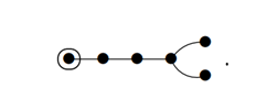
However, the only Tits index of rank \(2\) containing this one is, with the notation of [30], the index \(\mathsf{^2D_{7,2}^{(1)}}\). But the other rank 1 residue is just a projective line over \(\mathbb{K}\), which can never be the case for an ovoid of a polar space of rank 3 over \(\mathbb{K}\) (the arguments in [15, Section 6.4] show that this quadrangle is actually a subquadrangle induced by an extended equator geometry, and hence can never coincide with the complete Moufang quadrangle defined by the ideal Veronesean).
This completes the proof of the proposition. \(\square\)
We now deal with dualities of thick \(\mathsf{F}_4\) buildings, that is, we classify ovoidal subcomplexes of class 2 in \(\Delta\) under a mild additional condition (weaker than condition (WCC)). The result already includes the statement of Main Result 1.5(ii) for class 2 ovoidal subcomplexes with Weyl diagram \(\mathsf{^2F_{4;2}}\).
Theorem 4.33. Let \(\Delta\) be a thick building of type \(\mathsf{F_4}\) and let \(\Sigma\) be a subcomplex of the corresponding building. Then the following are equivalent
- (i) The subcomplex \(\Sigma\) is ovoidal of type \(\mathsf{^2F}_{4;2}\) and satisfies condition (WCC).
- (ii) The subcomplex \(\Sigma\) is ovoidal of type \(\mathsf{^2F}_{4;2}\) and for each pair of simplices \(\{v_1,v_{4}\}\), \(\{v_1′,v_4’\}\) of \(\Sigma\) of type \(\{1,4\}\) (where the index is the type) it holds that, if \(v_1\) and \(v_1’\) are opposite, then so are \(v_4\) and \(v_4’\).
- (iii) The subcomplex \(\Sigma\) defines a Moufang octagon, \(\Delta\) is self dual, and there exists a polarity of \(\Delta\) whose set of fixed simplices is precisely \(\Sigma\).
Proof. It is clear that (ii) follows from (i) and that (i) follows from (iii). Hence it remains to show that (iii) follows from (ii). So assume \(\Sigma\) is ovoidal of type \(\mathsf{^2F_{4;2}}\) satisfying the additional condition mentioned in (ii). Our first principal aim is to show that \(\Sigma\) defines a generalized octagon. The first subgoal is to prove that for each pair of simplices of \(\Sigma\) of type \(\{1,4\}\), the distance between the vertices of type \(1\) is the same as the distance between the vertices of type \(4\). For convenience we will work in the corresponding metasymplectic space of type \(\mathsf{F_{4,1}}\), where \(\Sigma\) is identified with a set of point-symp and line-plane pairs. We denote this space also by \(\Delta\). Note that the corresponding geometry of type \(\mathsf{F_{4,4}}\) is also a metasymplectic space, and we call it the dual of \(\Delta\), denoted by \(\Delta^*\). We will occasionally appeal to dual arguments. Also, we denote opposite object \(S,S’\) in \(\Delta\) as \(S\equiv S’\).
We prove some numbered claims so that we may easily refer to them.
Claim 1. Each pair \((\{p_1,\xi_1\},\{p_2,\xi_2\})\subseteq\Sigma\) of point-symp pairs, \(p_1,p_2\) points and \(\xi_1,\xi_2\) symps of \(\Delta\), has the property that, if \(\xi_1\) and \(\xi_2\) are opposite, then so are \(p_1\) and \(p_2\).
Indeed, choose such pairs with \(\xi_1\) and \(\xi_2\) opposite and suppose \(p_1,p_2\) are not opposite. First suppose that \(p_1\) and \(p_2\) are special. Let \(p_1’\) be the unique point of \(\xi_1\) symplectic to \(p_2\). We can find a line-plane pair \(\{L_1,\pi_1\}\in\Sigma\) incident with \(\{p_1,\xi_1\}\) and such that \(L_1\) is not collinear with \(p_1’\). Then all points of \(L_1\setminus\{p_1\}\) are opposite \(p_2\). There exists a unique symp \(\zeta_1\) through \(\pi_1\) not opposite \(\xi_2\). Since \(\Sigma\) is ovoidal, there exists a point \(x_1\in L_1\) such that \(\{x_1,\zeta_1\}\in\Sigma\). Since \(\zeta_1\neq\xi_1\), we have \(x_1\neq p_1\). Hence \(\{x_1,\zeta_1\}\) and \(\{p_2,\xi_2\}\) are not opposite while \(x_1,p_2\) are. This contradicts the assumption of (ii).
Now suppose \(p_2\) is symplectic to \(p_1\). On any line \(M_1\) through \(p_1\), which belongs to a line-plane pair \(\{M,\alpha_1\}\) in \(\Sigma\), we can find a point \(y_1\) such that the point-symp pair \(\{y_1,\eta_1\}\in\Sigma\) incident with \(\{M_1,\alpha_1\}\) has its symp \(\eta_1\) opposite \(\xi_2\). This contradicts the conclusion in the previous paragraph. We conclude that Claim 1 is proved.
Claim 1 implies that the assumptions are now self-dual. So from now on, we may appeal to the duality principle. We already do so for the next consequence and claim.
Consequence 1. If \(L,L’\) are lines, \(\pi,\pi’\) planes and \(\{L,\pi\},\{L’,\pi’\}\in\Sigma\), then \(L\) is opposite \(L’\) if, and only if, \(\pi\) is opposite \(\pi’\).
Indeed, by our previous remark it is enough to show one direction, since the other direction is the dual. Suppose \(L\equiv L’\) and suppose \(\pi\not\equiv\pi’\). Then some point \(x\in\pi\) is symplectic to some point \(x’\in\pi’\). There is a symplecton \(\zeta\) containing \(\pi\) and a line of \(\xi(x,x’)\). Clearly, \(\zeta\) is not opposite any symp through \(\pi’\), whereas there exists a point \(p\in L\) such that \(\{p,\zeta\}\in\Sigma\), and \(p\) is opposite at least one point of \(L’\), contradicting Claim 1. Consequence 1 is proved.
Claim 2. Each pair \((\{p_1,\xi_1\},\{p_2,\xi_2\})\subseteq\Sigma\) of point-symp pairs, \(p_1,p_2\) points and \(\xi_1,\xi_2\) symps of \(\Delta\), has the property that \(\xi_1\) and \(\xi_2\) are special if, and only if, \(p_1\) and \(p_2\) are special.
Indeed, suppose \(\xi_1\) and \(\xi_2\) are special, with \(\xi\) a symp sharing a plane \(\alpha_i\) with \(\xi_i\), \(i=1,2\). By assumption, \(p_1\) and \(p_2\) are not opposite. If they are special, there is nothing to prove, so suppose now first that they are symplectic. Then we may assume that \(p_1\in\alpha_1\). Suppose \(p_2\notin\alpha_2\). Then \(p_1^\perp\cap\alpha_2=p_2^\perp\cap \alpha_2=:L\). Since \(\Sigma\) is ovoidal, we find a line-plane pair \(\{L_2,\pi_2\}\in\Sigma\) with \(p_2\in L_2\) and \(\pi_2\) disjoint from \(\alpha_2\). Each symp through \(\pi_2\) distinct from \(\xi_2\) is opposite \(\xi_1\), whereas no point on \(L_2\) is opposite \(p_1\), a contradiction to Claim 1. Suppose now \(p_2\in \alpha_2\). Let \(K_i\) be the unique line through \(p_i\) in \(\alpha_i\) contained in a line-plane pair of \(\Sigma\), \(i=1,2\). Since lines contain at least three points, we can select a point \(x_1\in p_2^\perp\cap\alpha_1\) distinct from both \(K_2^\perp\cap\alpha_1\) and \(p_2^\perp\cap L_1\). Set \(M_1=p_1x_1\) and \(M_2=x_1^\perp\cap\alpha_2\). Setting \(i=1,2\), select a plane \(\beta_i\neq\alpha_i\) in \(\xi_i\) through \(M_i\), not belonging to a line-plane pair of \(\Sigma\) incident with \(\{p_i,\xi_i\}\). Then there is a unique line-plane pair \(\{N_i,\gamma_i\}\in\Sigma\) incident with \(\{p_i,\xi_i\}\) such that \(N_i\subseteq \beta_i\). Pick a point \(y_i\in N_i\setminus\{p_i\}\). Let \(\{y_i,\zeta_i\}\in\Sigma\) be incident with \(\{N_i,\gamma_i\}\). Then, since \(\zeta_1\cap\xi=p_1\) is symplectic to \(p_2=\zeta_2\cap\xi\), we find that \(\zeta_1\) is opposite \(\zeta_2\). However, \(y_1\) is collinear to \(x_1\), which is symplectic to \(y_2\), as \(M_2\subseteq x_1^\perp\cap y_2^\perp\). Hence \(y_1\) and \(y_2\) are not opposite, a contradiction to Claim 1 again.
Now suppose \(p_1\perp p_2\). Let \(K_i\) be as in the previous case and suppose first that \(p_i^\perp\cap\alpha_j=K_j\), \(\{i,j\}=\{1,2\}\). Then every point of \(K_1\setminus\{p_1\}\) is symplectic to every point of \(K_2\setminus\{p_2\}\). Define \(\{K_i,\beta_i\}\in\Sigma\) to be incident with \(\{p_i,\xi_i\}\), \(i=1,2\). For a given symp through \(\beta_1\) distinct from \(\xi\) (which is only relevant if \(\beta_1=\alpha_2\)), there is at most one symp through \(\beta_2\) not special to the given symp. Hence we can find points \(z_i\in K_i\setminus\{p_i\}\), \(i=1,2\), such that the unique symps \(\zeta_i\) with \(\{z_i,\zeta_i\}\in\Sigma\) incident with \(\{K_i,\beta_i\}\) are special. Since \(z_1\) and \(z_2\) are symplectic, that contradicts the previous paragraph.
Hence we may assume that \(K_1\neq p_2^\perp\cap\alpha_1:=K_1’\). There are a unique plane \(\gamma_1\) through \(K_1’\) in \(\xi_1\) and a unique line \(M_1\subseteq\gamma_1\) through \(p_1\) such that \(\{M_1,\gamma_1\}\in\Sigma\). Note that every point of \(M_1\setminus\{p_1\}\) is symplectic to \(p_2\), but only one symp through \(\gamma_1\) is symplectic to \(\xi_2\). Hence we can again find a simplex \(\{x_1,\zeta_1\}\in\Sigma\), with \(x_1\in M_1\setminus\{p_1\}\) and \(\gamma_1\subseteq\zeta_1\), and \(x_1\) symplectic to \(p_1\), while \(\zeta_1\) special to \(\xi_2\), again contradicting a previous paragraph.
Hence we have shown that, if \(\{p_1,\xi_1\},\{p_2,\xi_2\}\in\Sigma\) with \(p_1,p_2\) points and \(\xi_1,\xi_2\) symps of \(\Delta\), and \(\xi_1\) and \(\xi_2\) are special, then \(p_1\) and \(p_2\) are special as well. Since the converse is the dual, the proof of Claim 2 is complete.
Claim 3. Each pair \((\{p_1,\xi_1\},\{p_2,\xi_2\})\subseteq\Sigma\) of point-symp pairs, \(p_1,p_2\) points and \(\xi_1,\xi_2\) symps of \(\Delta\), has the property that \(\xi_1\) and \(\xi_2\) are symplectic if, and only if, \(p_1\) and \(p_2\) are symplectic.
Indeed, let \(\xi_1\) and \(\xi_2\) be symplectic, that is, they intersect in a unique point \(p\). If \(p_1=p=p_2\), then by considering an arbitrary point \(q_1\) on a line \(L_1\) such that \(\{L_1,\alpha_1\}\in\Sigma\) and \(p_1\in L_1\subseteq \alpha_1\subseteq\xi_1\), with \(q_1\) distinct from \(p_1\) and such that the unique symp \(\zeta_1\) with \(\{q_1,\zeta_1\}\in\Sigma\) and \(\alpha_1\subseteq\zeta_1\) is not adjacent to \(\xi_2\), we reduce this situation to \(p_1\neq p=p_2\). Then there exists a line-plane pair \(\{M_1,\beta_1\}\in\Sigma\) with \(p_1\in M_1\subseteq\xi_1\) but \(p\notin\beta_1\). Selecting an arbitrary point \(p_1’\in M_1\setminus p_1\), we see that the corresponding symp through \(\beta_1\) is special to \(\xi_2\), whereas \(p_1’\) is symplectic or collinear to \(p_2\), contradicting Claim 2.
So, we may assume that \(p_1\neq p\neq p_2\). We do have \(p_1\perp p\perp p_2\perp p_1\) as otherwise we contradict one of the previous claims. So, we can still choose \(p_1’\) as in the previous paragraph, now taking care that \(p_1’\) is not collinear to \(p\) and we denote the corresponding symp as \(\xi_1’\). We now choose \(\{p_2′,\xi_2’\}\) analogously, but with respect to \(p_2\) and \(\xi_2\). Then \(p_1’\) is opposite \(p_2’\), but the symps \(\xi_1’\) and \(\xi_2’\) contain collinear points \(p_1\) and \(p_2\), respectively, contradicting Claim 1. This proves Claim 3.
Claim 4. Each pair \((\{p_1,\xi_1\},\{p_2,\xi_2\})\subseteq\Sigma\) of point-symp pairs, \(p_1,p_2\) points and \(\xi_1,\xi_2\) symps of \(\Delta\), has the property that \(\xi_1\) and \(\xi_2\) are adjacent if, and only if, \(p_1\) and \(p_2\) are collinear. Moreover, if both conditions are satisfied, then \(p_1p_2\subseteq\xi_1\cap\xi_2\) and \(\{p_1p_2,\xi_1\cap\xi_2\}\in\Sigma\).
Indeed, suppose \(\xi_1\) and \(\xi_2\) are adjacent while \(p_1\) is not collinear to \(p_2\). Then, by the foregoing claims, \(p_1=p_2\). Then there exist a plane \(\alpha_1\) through \(p_1\) inside \(\xi_1\) intersecting \(\xi_1\cap\xi_2\) in exactly \(p_1\), and a line \(L_1\subseteq \alpha_1\) with \(p_1\in L_1\) such that \(\{L_1,\alpha_1\}\in\Sigma\). Let \(\{q_1,\zeta_1\}\in\Sigma\) be such that \(q_1\in L_1\setminus\{p_1\}\) and \(\alpha_1\subseteq \zeta_1\). Then \(\zeta_1\) and \(\xi_2\) intersect in exactly \(p_1=p_2\), but \(q_1\perp p_2\), contradicting Claim 3.
Hence \(p_1\perp p_2\), \(p_1\neq p_2\). Suppose \(p_1\notin\xi_2\). Then clearly \(p_2\in\xi_1\). There exist a plane \(\alpha_1\subseteq\xi_1\) with \(p_1\in\alpha_1\), and a line \(L_1\subseteq\alpha_1\) with again \(p_1\in L_1\), such that \(\{L_1,\alpha_1\}\in\Sigma\) and \(\alpha_1\cap\xi_2\) is empty. It is also easy to see that we can choose \(L_1\) not contained in \(p_2^\perp\). As before this yields \(\{q_1,\zeta_1\}\in\Sigma\) with \(p_1\neq q_1\in L_1\subseteq\alpha_1\subseteq\xi_1\). Then \(q_1\) is symplectic to \(p_2\), but \(\zeta_1\) is special to \(\xi_2\), contradicting Claims 2 and 3. Hence \(p_1p_2=:L\subseteq \alpha:=\xi_1\cap\xi_2\). Set \(i=1,2\). There exist a unique line \(L_i\subseteq\alpha\) and a unique plane \(\beta_i\) with \(p_i\in L_i\subseteq \beta_i\subseteq\xi_i\) and \(\{L_i,\beta_i\}\in\Sigma\). Suppose there exists \(p\in L_1\cap L_2\setminus L\). By the dual of the previous paragraph, there is a unique symp \(\xi\ni p\) with \(\{p,\xi\}\in\Sigma\), and it has to contain \(\beta_1\) and \(\beta_2\). This is only possible if at least one of \(\beta_1,\beta_2\) coincides with \(\xi_1\cap\xi_2\). But then \(\xi\) coincides with either \(\xi_1\) or \(\xi_2\), a contradiction. So we may assume \(L_1=L\). Then \(p_2\in L_1\) and so \(\beta_2\subseteq\xi_1\), implying \(\beta_2=\alpha\). But now, by the Weyl diagram, there exists a unique point \(q\in L_2\setminus\{p_2\}\) with \(\{q,\xi_2\}\in\Sigma\), contradicting the dual of the first paragraph again.
Now it follows that for each point-symp pair \(\{p,\xi\}\in\Sigma\), the symp \(\xi\) is uniquely determined by \(p\) and we write \(\xi=p^\sigma\) and \(p=\xi^\sigma\). A point (symp) in the domain of \(\sigma\) will be called a Ree point (symp). Similarly we define Ree lines and Ree planes, and for a Ree line \(L\), there is a unique plane \(L^\sigma\) such that \(\{L,L^\sigma\}\in\Sigma\). We also write \(L=(L^\sigma)^\sigma\).
Similar results as Claim 4 pinning down the mutual positions of pairs of point-symp pairs of \(\Sigma\) exist. We prove them now, going our way up from close to far. We will briefly call a pair of point-symp pairs of \(\Sigma\) collinear, symplectic, special, opposite, if the points of these pairs are collinear, symplectic, special, opposite, respectively.
Claim 5. If a pair \((\{p_1,\xi_1\},\{p_2,\xi_2\})\subseteq\Sigma\) of point-symp pairs, \(p_1,p_2\) points and \(\xi_1,\xi_2\) symps of \(\Delta\), is symplectic, then, writing \(p:=\xi_1\cap\xi_2\) and letting \(\xi\) be the symp containing \(p_1\) and \(p_2\), the pair \(\{p,\xi\}\) belongs to \(\Sigma\). Moreover, \(p_1\perp p\perp p_2\).
Indeed, assume first for a contradiction that \(p=p_1\). Similar arguments as before yield a Ree point \(q\perp p\) in \(\xi_1\) such that \(q^\sigma\) intersects \(\xi_2\) in exactly \(p\). Since \(q\) is special to \(p_2\) (noting that \(p_1\) and \(p_2\) are not collinear!), this contradicts Claim 2. Hence \(p_1\perp p\perp p_2\), with \(p_1\neq p\neq p_2\). Assume next for a contradiction that the line \(K_1:=pp_1\) is not a Ree line. Set \(L_1:=p_2^\perp\cap \xi_1\). Then, since \(p_1\) is symplectic to \(p_2\), we find \(L_1\subseteq p_1^\perp\). Set \(\beta_1:=\left\langle p_1,L_1\right\rangle\). Let \(\{M_1,\alpha_1\}\in\Sigma\) be incident with \(\{p_1,\xi_1\}\) such that \(M_1\subseteq\beta_1\). Set \(x=M_1\cap L_1\). Then, by Claim 4, \(x\in\xi_2\), a contradiction. Hence \(p\) belongs to a point-symp pair of \(\Sigma\) and, dually, \(p^\sigma=\xi\). Claim 5 is proved.
Claim 6. If a pair \((\{p_1,\xi_1\},\{p_2,\xi_2\})\subseteq\Sigma\) of point-symp pairs, \(p_1,p_2\) points and \(\xi_1,\xi_2\) symps of \(\Delta\), is special, then neither \(p_1\) nor \(p_2\) is contained in the unique symp \(\xi\) adjacent to both \(\xi_1\) and \(\xi_2\) (implying that \(\xi\) is not a Ree symp). Moreover, there exist unique Ree points \(q_1\) and \(q_2\) with \(p_1\perp q_1\perp q_2\perp p_2\).
Indeed, suppose first that \(p_1\in\xi\). Then \(p_2\notin \xi\) and we find a Ree point \(q_2\perp p_2\) in \(\xi\). If \(q_2\perp p_1\), then \(q_2\in p_1^\sigma=\xi_1\) by Claim 4, a contradiction. Hence \(q_2\) is symplectic to \(p_1\). Claim 5 yields a Ree point \(q\in\xi\) with \(q^\sigma=\xi\). Claim 4 again implies \(q\perp \xi_1\cap\xi_2\), a contradiction. Hence \(p_1\) is far from \(\xi_2\) and \(p_2\) is far from \(\xi_1\). We now also see that \(\xi\) is not a Ree symp, as by Claim 4 the point \(\xi^\sigma\) would have to belong to both \(\xi_1\) and \(\xi_2\), a contradiction. Dually, the unique point in \(\Delta\) collinear to both \(p_1\) and \(p_2\) is not a Ree point.
Let \(i=1,2\). Set \(\alpha_i=:\xi_i\cap\xi\) and \(L_i=:p_i^\perp\cap\alpha_i\). Since \(p_1\) is special to \(p_2\), there exists a unique point \(r_i\in L_i\cap L_{3-i}^\perp\). We find a Ree point \(q_i\in L_i\) on the unique Ree line contained in \(\left\langle p_i,L_i\right\rangle\). If \(q_1\) is symplectic to \(q_2\), then \(\xi\) is a Ree symp by Claim 5, contradicting our previous observation. So \(q_1\perp q_2\) and we may assume without loss of generality that \(q_1=r_1\). If \(q_2\neq r_2\), then \(q_2\) is special to \(p_1\), with \(q_2\perp q_1\perp p_1\). This contradicts our earlier observation that the unique point collinear to two special Ree points is not a Ree point. Hence \(r_1\) and \(r_2\) are both Ree points. Clearly, the sequence \((p_1,r_1,r_2,p_2)\) is unique as every other Ree point collinear to \(p_1\) is either special to or opposite \(p_2\), and so only longer sequences can occur. Claim 6 is proved.
Before we prove that we actually have a generalized octagon, we make a couple of observations.
Observation 4.34. Let \(p_1,p_2\) be two Ree points. If \(p_1\perp p_2\), then every Ree point collinear to \(p_2\), but not on the line \(p_1p_2\), is symplectic to \(p_1\).
Indeed , if \(q\perp p_2\) is a Ree point not on \(p_1p_2\), then it lies in \(p_2^\sigma\) and the axioms of an ovoidal subcomplex of type 2 imply the assertion.
Observation 4.35. Let \(p_1,p_2\) be two Ree points. If \(p_1\) is symplectic to \(p_2\), then there is a unique Ree point \(p\) collinear to both \(p_1,p_2\), and every Ree point collinear to \(p_2\), but not lying on the line \(p_2p\), is special to \(p_1\).
Indeed, Claim \(5\) proves the existence of \(p\) and the uniqueness of \((p^\sigma)^\sigma\) proves the uniqueness of \(p\) (if \(q\) would be another Ree point collinear with both \(p_1,p_2\), then \(q^\sigma\) contains \(p_1,p_2\) and hence coincides with \(p^\sigma\)). Now let \(p_3\perp p_2\) be a Ree point not on \(p_2p\). In \(p_2^\sigma\), the point \(p_3\) is not collinear to \(p\), which means that \(p_3^\perp\cap p^\sigma\) is not contained in \(p_1^\perp\). This implies that \(p_3\) is special to \(p_1\).
Observation 4.36. Let \(p_1,p_2\) be two Ree points. If \(p_1\) is special to \(p_2\), then there are unique Ree points \(q_1,q_2\) with \(p_1\perp q_1\perp q_2\perp p_2\), and every Ree point \(p_3\) collinear to \(p_2\), but not on the line \(p_2q_2\), is opposite \(p_1\). Also, \(q_1\) is the unique point of \(p_1^\sigma\) symplectic to \(p_2\).
The first part of this observation is contained in Claim 6. The second part follows from the construction of \(q_1,q_2\) and an argument similar to the one used in the proof of Observation 4.35. The last assertion follows directly from the proof of Claim 6.
We are now ready to prove our first principal goal.
Claim 7. The set of Ree points, furnished with the Ree lines, is a generalized octagon.
We denote the geometry of Ree points and Ree lines as \(O_R\). Observation \(1\) implies that there are no triangles in \(O_R\), and that every pair of points in \(O_R\) at mutual distance 2 are symplectic in \(\Delta\). Observation 4.35 implies that there are no quadrangles in \(O_R\) and, combined with Claim 6, it implies that there are no pentagons in \(O_R\). If also follows that points in \(O_R\) are at mutual distance \(3\) if, and only if, they are special in \(\Delta\). Claim 6 then implies that there are no hexagons in \(O_R\). Observation 4.36 now implies that there are no heptagons in \(O_R\) (as two points at distance 3 in such a heptagon should at the same time be special — considering the path of length 3 connecting them — and opposite — considering the path of length 4 connecting them — in \(\Delta\), a contradiction). It suffices to show that every line contains a point at distance at most \(3\) from a given point. Let \(p\) be a Ree point and \(L\) be a Ree line. Then \(L\) contains at least one (Ree) point not opposite \(p\) in \(\Delta\). Such a point is at distance at most \(3\) from \(p\) by our previous findings. Claim 7 is proved.
Next we want to prove our second principal aim, that is, \(O_R\) is a Ree-Tits octagon. For that, we have to prove the Moufang property for \(O_R\). To do so, it is convenient to first show that \(\Sigma\) is a convex chamber complex of \(\Delta\).
Claim 8. The complex \(\Sigma\) is convex in \(\Delta\).
This is equivalent to showing that \(\Sigma\) is closed under projection. Let \(p_1\) and \(p_2\) be two Ree points and let \(\{p_i,\xi_i\}\), \(i=1,2\), be the corresponding simplices of \(\Sigma\). First suppose that \(p_1\) and \(p_2\) are collinear. Then both those simplices are contained in a chamber of \(\Delta\) together with the simplex \(\{p_1p_2,\xi_1\cap\xi_2\}\), which belongs to \(\Sigma\). Hence the projection of \(\{p_1,\xi_1\}\) onto \(\{p_2,\xi_2\}\) is the chamber \(\{p_1,p_1p_2,\xi_1\cap\xi_2,\xi_2\}\), which also defines a chamber of \(\Sigma\).
Now suppose that \(p_1\) is symplectic to \(p_2\). By Claim 5, the simplex \(\{\xi_1\cap\xi_2,\xi(p_1,p_2)\}\) belongs to \(\Sigma\) and defines a Ree point collinear to both \(p_1,p_2\). Setting \(p:=\xi_1\cap\xi_2\) and \(\xi:=\xi(p_1,p_2)\), we see that the individual projections of \(p_2\) and \(\xi_2\) onto \(\{p_1,\xi_1\}\) in \(\Delta\) are \(\{p_1,\xi_1\cap\xi,\xi_1\}\) and \(\{p_1,p_1p,\xi_1\}\), respectively. Hence the projection of \(\{p_2,\xi_2\}\) onto \(\{p_1,\xi_1\}\) equals \(\{p_1,p_1p,\xi_1\cap\xi,\xi_1\}\). Since \(\{p_1p,\xi_1\cap\xi\}\in\Sigma\), the claim follows in this case.
Now assume \(p_1\Join p_2\). Let \(r_1,r_2\) be the unique Ree points with \(p_1\perp r_1\perp r_2\perp p_2\). The second paragraph of the proof of Claim 6 implies that the projection of \(\xi_2\) onto \(\{p_1,\xi_1\}\) is \(\{p_1,\left\langle p_1,r_2^\perp\cap\xi_1\right\rangle,\xi_1\}\). Similarly, the projection of \(p_2\) onto \(\{p_1,\xi_1\}\) is \(\{p_1,p_1r_1,\xi_1\}\). The claim now again follows.
Now let \(\{L_i,\pi_i\}\in \Sigma\), with \(L_i\) Ree lines and \(L_i^\sigma=\pi_i\), \(i=1,2\). If \(L_1\) and \(L_2\) meet, then \(p:=L_1\cap L_2\) is a Ree point and clearly, by uniqueness of \(p^\sigma\), the latter is the symp containing \(L_1\) and \(L_2\), which also contains \(\pi_1\) and \(\pi_2\). It fiollows that the projection of \(\{L_2,\pi_2\}\) onto \(\{L_1,\pi_1\}\) is equal to \(\{p,L_1,\pi_1,p^\sigma\}\) and the claim follows.
Now suppose \(L_1\) and \(L_2\) do not meet, but there are collinear Ree points \(p_i\in L_i\), \(i=1,2\). Observation 4.34 implies that every point on \(L_1\setminus\{p_1\}\) is symplectic to \(p_2\) and Observation 4.35 then implies that every such point is special to every point of \(L_2\setminus\{p_2\}\). Hence \(p_1\) is the projection of \(L_2\) onto \(\{L_1,\pi_1\}\). Likewise, \(p_1^\sigma\) is the projection of \(\Pi_2\) onto \(\{L_1,\pi_1\}\) and the claim again follows.
The proof for \(L_1\) and \(L_2\) not meeting and not containing collinear points, but a pair of symplectic points is completely similar.
The case where we project a point-symp pair \(\{p,\xi\}\in\Sigma\) onto a line-plane pair \(\{L,\pi\}\) is easy: there is always a unique point \(q\in L\) nearest to \(p\) and, dually, a unique symp \(\zeta\supseteq\pi\) nearest to \(\xi\). It follows from earlier observations that \(\{q,\zeta\}\) belongs to \(\Sigma\), which shows the claim once again.
Finally, if we project a line-plane pair \(\{L,\pi\}\in \Sigma\) onto a point-symp pair \(\{p,\xi\}\in\Sigma\), then that is equivalent to projecting the projection \(\{q,L,\pi,\zeta\}\) of \(\{p,\xi\}\) onto \(\{L,\pi\}\), onto \(\{p,\xi\}\), which coincides with the projection of \(\{q,\zeta\}\) onto \(\{p,\xi\}\) because this projection is a chamber in \(\Delta\), and which was proved to belong to \(\Sigma\) before.
This completes the proof of Claim 8. In the next claim we freely use the terminology of [16].
Claim 9. The generalised octagon \(O_R\) is a Moufang octagons and all elations are induced by unipotent elements of \(\mathsf{Aut}(\Delta)\).
By Claim 8, \(\Sigma\) is a thick twisting of \(\Delta\) in the sense of [16, §3]. Since each incident point-line pair in \(O_R\) defines a unique chamber of \(\Delta\), it is also a thick folding of Type 3 in the sense of [16, §2], which can be seen by considering an apartment through two opposite chambers of \(O_R\). Then by either Proposition 2.8 or 3.1 of [16], \(O_R\) is a Moufang octagon. Also, [16, Lemma 2.7] now shows that elations are induced by unipotent elements of \(\Delta\). Note that Lemma 2.7 of [16] holds for both thick foldings and thick twistings, but it is only explicitly proved in [16] for foldings; the proof for twistings is completely similar, as noted in [16, §3]. This completes the proof of Claim 9.
Our final principal aim is to show that \(\Sigma\) is the fixed complex of a polarity of \(\Delta\). Let \(P:=\{p,\xi\}\in\Sigma\), with \(p\) a Ree point. Then \(\mathop{\mathrm{\mathsf{Res}}}_\Delta(P)\), which is equal to \(\mathop{\mathrm{\mathsf{Res}}}_\xi(p)\), is a generalised quadrangle, which we denote as \(\Gamma\). The simplices of \(\Sigma\) incident with \(P\) define an ovoid-spread pairing \(\beta:\mathcal{O}\to\mathcal{S}\), with \(\mathcal{O}\) an ovoid of \(\Gamma\), \(\mathcal{S}\) a spread, and \(\beta\) a bijection.
Claim 10. Let \(x_i\in\mathcal{O}\), \(i=1,2,3\). Then the unique points on \(x_1^\beta\) collinear to \(x_2\) and \(x_3\), respectively, coincide, if, and only if, the unique lines through \(x_1\) concurrent with \(x_2^\beta\) and \(x_3^\beta\), respectively, coincide.
Let \((x_i,x_i^\beta\}\) be arbitrary, with \(x_i\in\mathcal{O}\), \(i=1,2,3\). Then Claim 9 implies that there exists a unipotent element \(\varphi\) of \(\Gamma\) fixing \(x_1\) and \(x_1^\beta\) and mapping \((x_2,x_2^\beta)\) to \((x_3,x_3^\beta)\). Moreover, varying \(x_3\), the set of all such unipotent elements constitutes a root group \(U\) of a (generalised) Suzuki group \(G\) (see [34]). Note that, if \(\mathbb{K}\) is finite, then the fact that no ovoids exist in generalised quadrangles with \(q+1\) points per line and \(q^2+1\) lines per line pencil, implies that \(\Delta\) is split. We assume that, if \(\Delta\) is finite, it is not defined over \(\mathbb{F}_2\), that is, \(\Gamma\) is not isomorphic to the smallest (thick) generalised quadrangle. Then \(U\) is nilpotent of class 2, and the centre \(Z(U)\) consists precisely of the involutions of \(U\) (plus the identity, of course), and is generated by all commutators (see [34]). Let \(U\) fix the point \(x\) and the line \(L\ni x\), with \(x\in\mathcal{O}\) and \(L=x^\beta\). By the classification of buildings of type \(\mathsf{F_4}\) (see Chapter 9 of [31]), the action of \(U\) induced on \(L\) is isomorphic to the action of the additive group of an alternative division algebra, and the same holds for the action of \(U\) induced on the line pencil of \(\Gamma\) at \(x\). Note that these actions are that of an elementary abelian \(2\)-group. Hence each commutator in \(U\) pointwise fixes \(L\) and linewise fixes \(x\). It follows that each member of \(Z(G)\) pointwise fixes \(L\) and linewise fixes \(x\). Suppose now some member \(u\in U\) linewise fixes \(x\). Then \(u\) induces on each of these lines an involution (for the same reason as before) and so \(u^2\) pointwise fixes \(x^\perp\). Since every member of \(\mathcal{S}\) distinct from \(L\) contains a unique point of \(x^\perp\), each member of \(\mathcal{S}\) is fixed by \(u^2\) and hence \(u^2\) is the identity, showing \(u\in Z(U)\), and hence \(u\) pointwise fixes \(L\). Conversely one shows that, dually, if \(u\in U\) pointwise fixes \(L\), then it linewise fixes \(x\).
Now let \(\{x_2,x_2^\beta\}\) and \(\{x_3,x_3^\beta\}\) be two members of the ovoid-spread pairing, distinct from \(\{x,L\}\) (with \(x_2,x_3\in\mathcal{O}\)). Suppose \(x_2\) and \(x_3\) are collinear to the same point \(p\) on \(L\). Let \(u\in U\) be the unique unipotent element mapping \(\{x_2,x_2^\beta\}\) onto \(\{x_3,x_3^\beta\}\). Then \(u\) fixes \(x\) and \(p\) on \(L\) and hence fixes \(L\) pointwise. It follows that \(u\) fixes \(x\) linewise, and consequently \(x_2^\beta\) intersects the same line through \(x\) as \(x_3^\beta\). The converse is shown dually.
Now suppose that \(\Delta\) is defined over \(\mathbb{F}_2\). Then a straight forward check reveals that the previous property is true for every possible ovoid-spread pairing in the smallest generalised quadrangle (use the fact that three points of an ovoid never occur as the intersection of two point perps and, dually, no three lines of any spread form one regulus of a \(3\times3\) grid. This completes the proof of Claim 10.
Now we define the following map \(\rho\) on \(\Gamma\). Each point \(x\in\mathcal{O}\) is mapped onto \(x^\beta\) and each line\(L\) of \(\mathcal{S}\) is mapped onto the point \(x\) for which \(x^\beta=L\). Now let \(p\) be some point with \(p\notin\mathcal{O}\). Then \(p\) is contained in a unique spread line \(x^\beta\in\mathcal{S}\). Let \(y\in \mathcal{O}\) be collinear to \(p\), but distinct from \(x\). Then there is a unique line through \(x\) intersecting \(y^\beta\). That line is by definition \(p^\rho\). By Claim 10, this is independent of \(y\perp p\), \(y\in\mathcal{O}\). Dually, one defines the image \(L^\rho\) of any line \(L\) of \(\Gamma\).
Claim 11. The map \(\rho\) is a polarity of \(\Gamma\).
Indeed, a moment’s thought reveals that, with the foregoing notation and convention, the image of \(p^\rho\) is precisely \(p\). Hence \(\rho\) is an involution. If \(L\) is an arbitrary line through \(p\), then we can choose the point \(y\in\mathcal{O}\) on \(L\), and we see that \(L^\rho\) is the projection of \(x\) onto \(y^\beta\), which belongs to \(p^\rho\). We conclude that \(\rho\) preserves incidence, and since it is an involution, it also preserves non-incidence. This means that \(\rho\) is a polarity, as we had to show. Claim 11 is proved.
To emphasise the dependence of \(\rho\) from \(x\), we sometimes also denote \(\rho\) as \(\rho_x\). Also, we sometimes view \(\rho_x\) as a map between the lines and planes through \(x\), in the obvious way.
Claim 12. Let \(\{L,\pi\}\in\Sigma\) consist of a line \(L\) and a plane \(\pi\). Then there exists a unique isomorphism \(\psi\) from the projective plane \(\pi\) to the residue \(\mathop{\mathrm{\mathsf{Res}}}_\Delta(L)\) such that, for each line \(K\subseteq \pi\), we have \(K^\psi=K^{\rho_x}\), with \(x=K\cap L\), and for each \(x\in L\), we have \(x^\psi=x^\sigma\).
Indeed, we can define the image \(K^\psi\) of any line \(K\) in \(\pi\) as \(K^\sigma\) if \(K=L\), and as \(K^{\rho_x}\) if \(K\neq L\) and \(x=K\cap L\). We have to show that triples of lines intersecting at a unique point \(p\) are mapped onto triples of planes contained in a common symp \(\xi_p\). If one of these lines is \(L\), then all images are contained in \(p^\sigma\). Assume now that \(p\in\pi\setminus L\) and let \(K_1,K_2,K_3\) be three lines in \(\pi\) through \(p\). Denote their respective intersection points with \(L\) as \(x_1,x_2,x_3\). Select an arbitrary plane \(\alpha_i\) through \(K_i\) in \(x_i^\sigma\), not containing \(L\), and let \(L_i\) be the Ree line in \(\alpha_i\), \(i=1,2\). Let \(y_4\) be a Ree point opposite \(x_2\) but symplectic to some point \(y_2\in L_1\) and let \(x_1\perp y_2\perp y_3\perp y_4\) be the unique path of Ree points joining \(x_1\) and \(y_4\) (cp. Claim 6). Let \(u\) be the automorphism of \(\Delta\) inducing the root elation in \(\Gamma\) that pointwise fixes the lines \(x_1y_2\), \(y_2y_3\) and \(y_3y_4\), that fixes all Ree lines through the points \(x_1, y_2, y_3\) and \(y_4\), and that maps \(\{x_2,x_2^\sigma\}\) to \(\{x_3,x_3^\sigma\}\).
We show that \(p\) is collinear with \(L_2^u\). Equivalently, we show that \(p\) is fixed by \(u\). Since \(\pi\) is stabilised by \(u\), it suffices to show that the line \(y_2p\) (which is indeed a line as \(y_2\in L_1\subseteq\alpha_1\) and \(p\in K_1\subseteq\alpha_1\)) is fixed. Therefore, we determine the action of \(u\) on the residue \(\mathop{\mathrm{\mathsf{Res}}}_\Delta(y_2)\). We view this residue as a polar space \(\Omega\) with point set the set of symps through \(y_2\), line set the set of planes through \(y_2\) and plane set the set of lines through \(y_2\), with natural incidence. The symp \(y_2^\sigma\) is a fixed point \(a\) of \(\Omega\). Moreover, \(u\) elementwise fixes the ovoid-spread pairing of \(\mathop{\mathrm{\mathsf{Res}}}_\Delta(\{y_2,y_2^\sigma\})\) induced by \(\Sigma\), which easily implies that \(u\) acts as the identity on the lines of \(\Omega\) through \(a\). The Ree planes through \(y_2\) correspond to an ovoid \(\mathcal{O}_a\) in \(\mathop{\mathrm{\mathsf{Res}}}_\Omega(a)\) of lines through \(a\). Now, the commutation relation in Ree-Tits octagons numbered (8M7) in Section 5.4.5 of [35] immediately implies that \(u\) fixes all points on each line of \(O_R\) through either \(y_2\) or \(y_3\). This, in turn, implies that each point of each line belonging to \(\mathcal{O}_a\) is fixed. Now, since \(x_1\) and \(y_4\) are fixed, the special pair of symps \(\{x_1^\sigma,y_4^\sigma\}\) is fixed, and hence so is the unique symp \(\zeta\) adjacent to both of these symps. Noticing that \(\zeta\) is not a Ree symp by Claim 6, this induces an additional fixed point in \(\Omega\) collinear to \(a\), but not on one of the pointwise fixed ovoid lines. This implies that all points of \(\Omega\) collinear to \(a\) are fixed. Finally, since all Ree lines through \(y_4\) and \(y_3\) are stabilised, the plane \((y_3y_4)^\sigma\) is pointwise fixed (project the aforementioned Ree lines onto it to see this quickly). Hence every line through \(y_2\) meeting that plane is stabilised, implying in \(\Omega\) that some planes not through \(a\) are stabilized. Consequently \(\mathop{\mathrm{\mathsf{Res}}}_\Delta(y_2)\) is elementwise fixed, implying that the line \(y_2p\) is fixed, and so, \(p\) is fixed, which we wanted to show.
Noticing that \(p\) is the unique point collinear to both \(y_2\) and some arbitrarily chosen \(z_2\in L_2\setminus\{x_2\}\), the dual token shows that the unique symp \(\xi^*\) adjacent to both \(y^2\) and \(z_2\) is stabilised by \(u\). But \(\xi^*\) contains \(K_1^\psi\) and \(K_2^\psi\). Hence it also contains \((K_2^\psi)^u=K_3^\psi\).
Now Claim 12 follows.
We are finally in a position to prove that there exists a polarity with fixed structure \(\Sigma\). To that aim, consider two opposite flags of \(O_R\), that is, two chambers \(C:=\{x,L,\pi,\xi\}\) and \(C’:=\{x’,L’,\pi’,\xi’\}\) with \(\{x,\xi\},\{x’,\xi’\},\{L,\pi\},\{L’,\pi’\}\in\Sigma\) and \(x\) opposite \(x’\) and \(L\) opposite \(L’\). Then \(C\) is opposite \(C’\) by Claim 1 and Consequence 1. Hence they determine a unique apartment \(\mathcal{A}\). The map \(\rho_x\) is a duality of \(\mathop{\mathrm{\mathsf{Res}}}_\Delta(\{x,\xi\}\). Furthermore, by Claim 12, there exists an isomorphism \(\psi\) from \(\mathop{\mathrm{\mathsf{Res}}}_\Delta(\{\pi,\xi\}\) to \(\mathop{\mathrm{\mathsf{Res}}}_\Delta(\{p,L\})\) compatible with \(\rho_x\) and such that elements of \(\mathcal{A}\) are mapped onto elements of \(\mathcal{A}\). The inverse of that isomorphism has the dual properties. The fact that elements of \(\mathcal{A}\) are mapped onto elements of \(\mathcal{A}\) means that both \(\rho_x\) and \(\psi\) (and also \(\psi^{-1}\)) are compatible with the duality of \(\mathcal{A}\) induced by the involution \[p\leftrightarrow\xi, \ \ \ p’\leftrightarrow\xi’, \ \ \ L\leftrightarrow \pi, \ \ \ L’\leftrightarrow\pi’.\]
We can now apply Tits’ extension theorem [31, Theorem 4.16] to obtain a polarity \(\theta\) of \(\Delta\) fixing all members of \(\Sigma\) incident with either \(\{p,\xi\}\) or \(\{L,\pi\}\), and fixing \(\{p’,\xi’\}\) and \(\{L’,\pi’\}\). The convexity of \(\Sigma\) readily implies that \(\Sigma\) is fixed elementwise. Since the fix structure of a polarity, hence also of \(\theta\), defines a generalised octagon \(O_\theta\), and clearly \(O_R\) is a subpolygon of \(O_\theta\), which is full by considering \(L\), and ideal by considering \(p\), [35, Theorem 1.8.2] yields \(O_R=O_\theta\).
The theorem is proved. \(\square\)
We now prove Proposition 1.3, which we recall first.
Proposition 4.37. Let \(A\) be the set of absolute points of a polarity \(\rho\) of a metasymplectic space \(\mathsf{F_{4,1}}(\mathbb{K},\mathbb{K}’)\). Then every duality for which every point of \(A\) is absolute coincides with \(\rho\). Also, every collineation of \(\mathsf{F_{4,1}}(\mathbb{K},\mathbb{K}’)\) pointwise fixing \(A\) is the identity.
Proof. We begin with the last assertion. Let \(\theta\) be a collineation of \(\mathsf{F_{4,1}}(\mathbb{K},\mathbb{K}’)\) fixing \(A\) pointwise. Let \(x\) be an arbitrary point of \(A\). Then the symp \(\xi=x^\rho\) intersects \(A\) in the lines through \(x\) of an ovoid \(O\) of \(\mathop{\mathrm{\mathsf{Res}}}_\xi(x)\), a so-called Suzuki-Tits ovoid (see Lemma 2 of Section 2.5 in [35]). We now claim that \(\theta\) pointwise fixes \(\mathop{\mathrm{\mathsf{Res}}}_\xi(x)\). If \(|\mathbb{K}|=|\mathbb{K}’|=2\), this is immediate. Otherwise [35, Theorem 7.6.10] implies that \(\theta\) fixes all lines of the corresponding spread \(\mathcal{S}\) of \(\mathop{\mathrm{\mathsf{Res}}}_\xi(x)\). Since each point of each member of \(\mathcal{S}\) is collinear to some member of \(O\), each member of \(\mathcal{S}\) is fixed pointwise by \(\theta\). Since \(\mathcal{S}\) is a spread, the claim follows.
Now select a point \(y\in A\) opposite \(x\); then the unique point \(y_0\in\xi\) symplectic to \(y\) is fixed by \(\theta\). As \(y_0\) is opposite \(x\) in \(\xi\), the previous claim then shows that \(x^\perp\cap y_0^\perp\) is fixed pointwise, and hence every line through \(y_0\) in \(\xi\) is stabilised. Since each line of \(\xi\) through \(y_0\) is opposite (opposition in the polar space \(\xi\)) at least one member of \(O\) in \(\xi\), the set \(y_0^\perp\cap\xi\) is fixed pointwise. Likewise, \(x^\perp\cap\xi\) is fixed pointwise and this readily implies that \(\xi\) is fixed pointwise. Dually, all lines through \(x\) are fixed. Similarly, all lines through \(y\) are fixed. This, in turn, implies that the equator geometry \(E(x,y)\) is fixed pointwise. It is easy to see that \(E(x,y)\) contains two opposite points \(a,b\in A\). Since also \(E(a,b)\) is fixed pointwise, [15, Lemma 5.1.5(iii)] concludes the proof of the last assertion of the statement.
Now let \(\rho’\) be a duality with the property that each point of \(A\) is absolute. We first claim that, if \(x,x’\in A\) are collinear, then \(\zeta:=x^{\rho’}\) or \(\zeta’:={x’}^{\rho’}\) contains the line \(xx’\). Indeed, suppose not, then, since \(\zeta\cap\zeta’\) is a plane, the point \(x\) is collinear to a line of that plane and to \(x’\), a contradiction. The claim follows.
Now let \(L\) be a line, all points of which belong to \(A\). We may assume \(x,x’,x”\in L\). If \(x^{\rho’}\) does not contain \(L\), then both \({x’}^{\rho’}\) and \({x”}^{\rho’}\) do by the previous claim. Since \(\rho’\) is a duality, \(x^{\rho’}\) also contains \(L\).
Now it follows easily that \(x^{\rho’}=x^\rho\), since both are apparently determined by the lines contained in \(A\) and containing \(x\). Since \(x\in A\) was arbitrary, it follows that \(a^{\rho’}=a^\rho\) for all \(a\in A\) so that \(a^{\rho’\rho}=a\) for all \(a’ \in A\). From the last assertion, proved above, we now deduce \(\rho’\rho=\mathrm{id}\), implying \(\rho=\rho’\). The proposition is proved. \(\square\)
Exceptional type \(\mathsf{E_7}\)
Here we deal with the case of buildings of type \(\mathsf{E_7}\). Such a building is, by [31], defined by a(n arbitrary) commutative field \(\mathbb{K}\), and we denote the building by \(\Delta=\mathsf{E_7}(\mathbb{K})\). With standard Bourbaki labelling of the vertices [19], we will mainly be focusing on the \(1\)-Grassmannian \(\mathsf{E_{7,1}}(\mathbb{K})\), which is the long root subgroups geometry and which we will also denote by \(\Delta\) (without causing confusion), and to a lesser extent the \(7\)-Grassmannian \(\mathsf{E_{7,7}}(\mathbb{K})\), also sometimes referred to as the “minuscule” geometry of type \(\mathsf{E_7}\). Since \(\Delta\) is a long root subgroup geometry, it shares many properties with metasymplectic spaces. However, there are also important differences. Here is a list of some basic properties that we will use. Again these can be read off the diagram if no reference is given.
The symps of \(\Delta\) are hyperbolic polar spaces \(\mathsf{D_{5,1}}(\mathbb{K})\) and correspond to vertices of type \(6\) of the building.
Each pair of distinct points is either collinear, symplectic, special or opposite.
Given a point \(p\) and a symp \(\xi\), there are the following possibilities: \(p\in\xi\), \(p\) collinear to (all points of) a line of \(\xi\), \(p\) collinear to a \(4’\)-space (using the same convention as in the \(\mathsf{E_6}\) case), \(p\) symplectic to all points of a unique \(4\)-space of \(\xi\), \(p\) symplectic to a unique point of \(\xi\).
The vertices of type \(7\) of the corresponding building define convex subspaces isomorphic to the geometry \(\mathsf{E_{6,1}}(\mathbb{K})\). We call them paras.
The \(4\)-spaces and the \(4’\)-spaces of a symp form its two natural systems of maximal singular subspaces.
We have the following point-para relation: if \(p\) is a point and \(\Pi\) a para, then either \(p\in\Pi\), \(p\) is collinear to a \(5\)-space of \(\Pi\), or there exists a unique para \(\Pi’\) through \(p\) intersecting \(\Pi\) in a symp (see e.g. [8, Fact 3.13(i)]).
We now introduce the Weyl substructures in \(\Delta\). There are two kinds.
- (1) An ideal fully embedded metasymplectic space. This is a metasymplectic space \(\Gamma\) whose point set is a subset of the point set of \(\Delta=\mathsf{E_{7,1}}(\mathbb{K})\) such that the point set of each line of \(\Gamma\) coincides with the point set of some line of \(\Delta\), and with the following two properties.
- (i) Isometricity. Points of \(\Gamma\) are opposite in \(\Gamma\) if, and only if, they are opposite in \(\Delta\).
- (ii) Ideality. The symps through a given plane \(\alpha\) form a line spread in the component of \(\mathop{\mathrm{\mathsf{Res}}}_\Delta(\alpha)\) isomorphic to a projective space.
- (2) An ideal dual polar Veronesean. This is a polar space \(\Gamma\) whose points are certain points of \(\Delta\), whose planes are ideal Veroneseans of paras, such that the lines (which define unique symps) and planes (which define unique paras) of \(\Gamma\) through a given point \(p\) define an ideal subspace of corank 4 in \(\mathop{\mathrm{\mathsf{Res}}}_\Delta(p)\), viewed as polar space of type \(\mathsf{D_{6,1}}\)
The name “dual polar Veronesean” stems from the fact that, viewed in \(\mathsf{E_{7,7}}(\mathbb{K})\), this structure is a dual polar space, and, viewed in the ambient projective space \(\mathsf{PG}(55,\mathbb{K})\) of the standard representation of \(\mathsf{E_{7,7}}(\mathbb{K})\), it is a dual polar Veronese variety, as defined in [10]. For our purposes, it is more convenient to see it as a point set of \(\mathsf{E_{7,1}}(\mathbb{K})\), but of course, these approaches are equivalent.
The following theorem is proved in [17].
Proposition 4.38. Let \(\theta\) be a non-trivial automorphism of \(\mathsf{E_{7}}(\mathbb{K})\), for some field \(\mathbb{K}\). Then \(\theta\) is uniclass if, and only if, it is either anisotropic, or the fixed point structure of \(\theta\) induced in \(\mathsf{E_{7,1}}(\mathbb{K})\) is an ideal fully embedded metasymplectic space \(\mathsf{F_{4,1}}(\mathbb{K},\mathbb{L})\), with \(\mathbb{L}\) a quadratic extension of \(\mathbb{K}\), isometrically embedded as a long root subgroup geometry, or the fixed point structure of \(\theta\) induced in \(\mathsf{E_{7,1}}(\mathbb{K})\) is an ideal dual polar Veronesean.
Note that the two examples correspond to the opposition diagram \(\mathsf{E_{7;3}}\) and \(\mathsf{E_{7;4}}\), respectively, and to the fix diagrams \(\mathsf{E_{7;4}}\) and \(\mathsf{E_{7;3}}\), respectively. In the latter case, the projective plane determined by the ideal Veronesean is a quaternion plane, or a plane over an inseparable extension of degree 4 of \(\mathbb{K}\), in characteristic \(2\). We will call such a dual polar space briefly quaternion. Quaternion Veroneseans are characterized by the property that the ovoids of the host spaces are obtained by intersecting the corresponding quadrics with subspaces of the ambient projective spaces, see [18].
We now prove the equivalence of these Weyl substructures with the ovoidal subcomplexes satisfying (WCC) or another seemingly weaker condition. We begin with the ideal dual polar Veroneseans and ovoidal subcomplexes with Weyl diagram \(\mathsf{E_{7;3}}\). .
Proposition 4.39. Let \(\Delta\) be a building of type \(\mathsf{E_7}\) and let \(\Sigma\) be a subcomplex. Then the following are equivalent
- (i) The subcomplex \(\Sigma\) is ovoidal of class \(1\) with Weyl diagram \(\mathsf{E_{7;3}}\) and satisfies condition (WCC).
- (ii) The subcomplex \(\Sigma\) is ovoidal of class \(1\) with Weyl diagram \(\mathsf{E_{7;3}}\) and every pair of vertices \(v_1,v_6\) of \(\Sigma\) of type \(1\) and \(6\), respectively, that are not incident with a common vertex of type \(7\) are in general position (that is, the vertex of type \(6\) is incident with a vertex of type \(1\) opposite \(v_1\)).
- (iii) The subcomplex \(\Sigma\) is ovoidal of class \(1\) with Weyl diagram \(\mathsf{E_{7;3}}\) and no pair of vertices of type \(1\) is special.
- (iv) The subcomplex \(\Sigma\) defines an ideal dual polar Veronesean, which is quaternion.
Proof. We show the implications \((i)\implies(ii)\implies(iii)\implies(iv)\implies (i)\), the latter being immediate.
If a pair of vertices \(v_1,v_6\) of \(\Sigma\) of type \(1\) and \(6\), respectively, that are not incident with a common vertex of type \(7\), are not in general position, then there is either a type 2 or a type 3 vertex in the convex closure, a contradiction. This shows that (ii) follows from (i).
Now suppose the subcomplex \(\Sigma\) is ovoidal of class \(1\) with Weyl diagram \(\mathsf{E_{7;3}}\) and some pair of vertices \(p,q\) of type \(1\) is special. We argue in \(\mathsf{E_{7,1}}(\mathbb{K})\). Let \(L\) be the unique line through \(q\) containing a point collinear to \(p\). Lemma 4.10 yields a symp \(\xi\in\Sigma\) containing \(L\). Since \(\{p,q\}\) is special, \(\xi\) and \(p\) are not contained in a common para; since \(p\) is collinear to some point of \(L\), and hence of \(\xi\), the pair \(\{p,\xi\}\) is not in general position. This shows that (iii) follows from (ii).
Now let \(\Sigma\) be an ovoidal subcomplex with Weyl diagram \(\mathsf{E_{7;3}}\) such that no pair of vertices of type \(1\) of \(\Sigma\) is special. We again reason in the long root subgroup geometry \(\Delta:=\mathsf{E_{7,1}}(\mathbb{K})\).
We first claim that, for each point \(p\in\Sigma\), the residue \(\mathop{\mathrm{\mathsf{Res}}}_{\Sigma}(p)\) is an ideal subspace of corank 4 of \(\mathop{\mathrm{\mathsf{Res}}}_\Delta(p)\). Suppose this is not the case for some point \(p\). Then, by the weaker condition in Proposition 4.13, we find two symps \(\xi\) and \(\zeta\) through \(p\) belonging to \(\Sigma\), not contained in a common para, and having a plane \(\pi\) in common. Then points \(x\in\xi\) and \(y\in\zeta\) with \(|x^\perp\cap\pi\cap y^\perp|=1\) form a special pair, a contradiction. The claim is proved.
Next we claim that two points of \(\Sigma\) are never collinear. Indeed, suppose \(p\perp q\), with \(p,q\in\Sigma\). In \(\mathop{\mathrm{\mathsf{Res}}}_\Delta(p)\), the line \(pq\) represents a maximal singular subspace of the polar space with point set the paras through \(p\). Lemma 4.10 yields a para \(\Pi\in\Sigma\) containing \(p\) and \(q\). This contradicts the fact that the elements of \(\Sigma\) in \(\Pi\) constitute an ideal Veronesean. The claim is proved. In particular, the foregoing ideal Veronesean is quaternion since, looking in the residue of a point, we recover the elements of \(\Sigma\) as a subspace, hence as the intersection of the corresponding polar space with a subspace of the ambient projective space.
In view of Proposition 4.23 and the definition above, it remains to show that \(\Sigma\) defines a polar space, with point set the points of \(\Sigma\), and line set the point sets of \(\Sigma\) determined by the symps in \(\Sigma\). The non-degeneracy axioms of a polar space can easily be proved by the reader; we content ourselves with proving the main axiom, namely, the one-or-all axiom. Let \(p,\xi\in\Sigma\) be a point and symp, respectively. If \(p,\xi\) are contained in a common para, then every point \(q\in\Sigma\) contained in \(\xi\) is symplectic to \(p\) (remember it cannot be collinear). We claim that the symp \(\zeta\) defined by \(p\) and \(q\) belongs to \(\Sigma\). We prove this claim for arbitrary symplectic points \(p,q\in\Sigma\).
Suppose for a contradiction that \(\zeta\) does not belong to \(\Sigma\). Then Lemma 4.10 yields a para \(\Pi\) through \(p\) intersecting \(\zeta\) in a \(4\)-space. By the point-para relations, \(q\) is collinear to all points of a \(5\)-space \(W\) of \(\Pi\), and all points of \(\Sigma\) in \(\Pi\) are collinear to a \(3\)-space of \(W\). Since no point of \(W\) belongs to \(\Sigma\) (it would otherwise be collinear to \(q\)), no symp of \(\Sigma\) in \(\Pi\) intersects \(W\) in a \(4’\)-space. If a symp of \(\Sigma\) in \(\Pi\) were disjoint from \(W\), then it would be incident with a \(5\)-space opposite \(W\) in \(\Pi\), yielding a point of \(\Sigma\) in that symp collinear to only one point of \(W\), a contradiction. Hence there is a symp \(\xi^*\in\Sigma\) in \(\Pi\) intersecting \(W\) in a line \(L\). A point of \(\Sigma\) contained in a \(4\)-space of \(\xi^*\) that intersects \(L\) in just one point is only collinear to the latter point of \(W\), again a contradiction. We conclude that the claim holds. It follows that the one-or-all axiom holds for \(p\) and \(\xi\) contained in a common para.
Next, suppose \(p\) and \(\xi\) are not contained in a common para. Then \(\xi\) contains points special to \(x\) and there are three possibilities (point-symp relations):
- (1) The point \(p\) is collinear to a line \(M\) of \(\xi\). As before, the points of \(\Sigma\) contained in a \(4\)-space of \(\xi\) intersecting \(M\) in just a point are special to \(p\), a contradiction.
- (2) The point \(p\) is symplectic to the points of a unique \(4\)-space of \(\xi\) and special to all other points of \(\xi\). Then \(p\) is special to te point of \(\Sigma\) contained in a \(4’\)-space of \(\xi\) disjoint from the aforementioned \(4\)-space. This is again a contradiction.
- (3) The point \(p\) is symplectic to a unique point \(x\in\xi\), special to all points of \(\xi\) collinear to \(x\) and opposite the other points of \(\xi\). If \(x\) was not contained in \(\Sigma\), then \(p\) is special to the unique point of \(\Sigma\) contained in an arbitrary \(4\)-space of \(\xi\) through \(x\), a contradiction. Hence \(x\in\Sigma\) and one of our previous claims implies that \(op\) and \(x\) are contained in a common symp of \(\Sigma\).
This shows the one-or-all axiom and we conclude that \(\Sigma\) defines a quaternion ideal dual polar Veronesean. \(\square\)
Now we treat the case of ovoidal subcomplexes with Weyl diagram \(\mathsf{E_{7;4}}\).
Proposition 4.40. Let \(\Delta\) be a building of type \(\mathsf{E_7}\) and let \(\Sigma\) be a subcomplex. Then the following are equivalent
- (i) The subcomplex \(\Sigma\) is ovoidal of type \(\mathsf{E_{7;4}}\) and satisfies condition (WCC).
- (ii) The subcomplex \(\Sigma\) is ovoidal of type \(\mathsf{E_{7;4}}\) and every pair of vertices \(v_1,v_6\) of \(\Sigma\) of type \(1\) and \(6\), respectively, such that no vertex of type \(1\) adjacent to \(v_1\) is incident with \(v_6\), are in general position (that is, the vertex of type \(6\) is incident with a vertex of type \(1\) opposite \(v_1\)).
- (iii) The subcomplex \(\Sigma\) defines a full and isometric embedding of a metasymplectic space \(\mathsf{F_{4,1}}(\mathbb{K},\mathbb{L})\), for some quadratic extension \(\mathbb{L}\) of \(\mathbb{K}\), into the long root subgroup geometry \(\mathsf{E_{7,1}}(\mathbb{K})\) related to \(\Delta\) such that the elements of type \(6\) of \(\Sigma\) incident with an element \(v\) of type \(4\) define an ovoid \(O\) of the polar space of type \(\mathsf{D_3}\) obtained from the residue of \(v\) in \(\Delta\). The ovoid \(O\) arises as the intersection of that polar space with a subspace of dimension \(3\) in an ambient projective space.
Proof. We again show the implications \((i)\implies(ii)\implies(iii)\implies (i)\), the first implication being immediate.
Suppose \(\Sigma\) is as in (ii) and assume for a contradiction that, in \(\mathsf{E_{7,1}}(\mathbb{K})\), two symps \(\xi_1\) and \(\xi_2\) of \(\Sigma\) intersect in a point \(p\in\Sigma\) and there exists a symp \(\zeta\) intersecting \(\xi_i\) in a \(4\)-space \(U_i\), \(i=1,2\). Note that \(\{p\}=U_1\cap U_2\). We claim that we can find a point \(x\in\Sigma\) in \(\xi_1\) symplectic to \(p\). Indeed, since \(\Sigma\) is a chamber complex, we can find a plane \(\pi_1\) through \(p\) in \(\xi_1\) belonging to \(\Sigma\). By the Weyl diagram, all lines of \(\pi_1\) through \(p\), all points of these lines, and finally all lines of \(\pi_1\) belong to \(\Sigma\). let \(K_1\) be a line of \(\pi_1\) not through \(x\). Pick \(u_1\in K_1\). Then \(\mathop{\mathrm{\mathsf{Res}}}_\Sigma(\{u_1,K_1,\xi_1\})\) is an ovoid in \(\mathop{\mathrm{\mathsf{Res}}}_{\xi_1}(K_1)\). Hence we find a plane \(\pi_1’\) through \(K_1\) not collinear to \(\pi_1\). We infer that each point \(x\) of \(\pi_1’\setminus K_1\) belongs to \(\Sigma\) and is symplectic to \(p\). The claim follows. If \(x\) were collinear to a point \(x_2\in\xi_2\), then it would be collinear to at least all points of a line, which would yield a point \(y_2\) collinear to \(p\), implying by convexity of symps that \(y_2\in\xi_1\), contradictory to the fact that then \(y_2=p\) and so \(p\perp x\). Hence the condition in (ii) now says that \(x\) and \(\xi_2\) are in general position, implying that there is a point \(z_2\in\xi_2\) opposite \(x\). But any point \(u_1\) of \(U_1\) collinear to \(x\) is collinear (in \(\zeta\)) to a \(3\)-space in \(U_2\), which certainly contains a line collinear to \(z_2\). This implies that \(z_2\) is symplectic to \(u_1\perp x\), contradicting the opposition of \(x\) and \(z_2\). This shows that no pair of vertices of \(\Sigma\) of type \(6\) is special in a residue of a vertex of \(\Sigma\) of type \(1\). Proposition 4.19 now implies that the elements of \(\Sigma\) incident with a given point \(p\) of \(\Sigma\) form a Weyl substructure, in other words, they form a composition spread in \(\mathop{\mathrm{\mathsf{Res}}}_\Delta(p)\), viewed as a polar space (hence with point set the set of paras containing \(p\)).
Let \(X\) be the set of points in \(\Sigma\) and let \(\mathcal{L}\) be the set of lines in \(\Sigma\). We use Definition 2.1 to show that \(\Gamma=(X,\mathcal{L})\) is a metasymplectic space with thick symps. First we have to show that \(\Gamma\) is a parapolar space. To that aim, it is convenient to show the claim that, if two points of \(X\) are symplectic in \(\Delta\), then the unique symp they are contained in belongs to \(\Sigma\).
So let \(p,q\in X\) be symplectic in \(\Delta\). Suppose for a contradiction that the symp \(\xi\) through \(p\) and \(q\) does not belong to \(\Sigma\). Then, in the residue of \(q\), viewed as polar space \(\mathsf{D_{6,1}}(\mathbb{K})\), \(\xi\) is a line not belonging to the Weyl complex induced by \(\Sigma\) in \(\mathop{\mathrm{\mathsf{Res}}}_\Delta(q)\). Hence we can select a symp \(\zeta\) through \(q\) belonging to \(\Sigma\) and which, viewed as a line in \(\mathsf{D_{6,1}}(\mathbb{K})\), is special to \(\xi\). It then follows that \(p\) and \(\zeta\) are not in general position, and that \(p^\perp\cap\zeta\) is empty, a contradiction to (ii). Hence \(\xi\in\Sigma\). The claim is proved.
We now show that \(\Gamma\) is connected. To that aim, let \(x,y\) be two arbitrary points of \(\Sigma\). If \(x\) and \(y\) are opposite in \(\Delta\), then we can find a point on any line of \(\Sigma\) through \(y\) special to \(x\). Hence we may assume that \(x\) and \(y\) are not opposite. If they are collinear, then likewise we can find a line of \(\Sigma\) through \(y\) locally opposite the line \(xy\), and hence this line contains a point of \(\Sigma\) special to \(x\). So we may assume that \(x\) and \(y\) are special (if they are symplectic, they are connected by the unique symp through them, which belongs to \(\Sigma\) as shown above). Looking in \(\mathop{\mathrm{\mathsf{Res}}}_\Delta(y)\), it is easy to see now that there exists a symp \(\xi\in\Sigma\) through \(y\) not in general position with \(x\). Hence, by our assumption in (ii), \(x\) is collinear to a line \(L\) of \(\xi\), and it is symplectic to all points of \(\Sigma\) contained in \(\xi\) and in a maximal singular subspace containing \(L\). The connectivity of \(\Gamma\) is proved.
Now let \(x,y\) be two points of \(X\) at distance \(2\) from each other, joined by at least two paths of length \(2\) contained in \(\Sigma\). Consider one of these paths and let \(p\) be its middle point. Since \(\Sigma\) induces in \(\mathop{\mathrm{\mathsf{Res}}}_\Delta(p)\) a Weyl complex, which is convex, it follows that, if \(x\) and \(y\) were collinear in \(\Delta\), then they would also be collinear in \(\Gamma\). Hence they are symplectic and the unique symp \(\xi\) containing both belongs to \(\Sigma\), by a previous claim we proved. Since \(\xi\) is convex in \(\Delta\), the convex closure of \(x,y\) in \(\Gamma\) is contained in \(\xi\). Since the points and lines of \(\Gamma\) form a polar space \(\Gamma_\xi\) of rank 3 in \(\xi\), that polar space is the convex closure. Note that \(\Gamma_\xi\) is thick. This verifies (i) of Definition 2.1. Now assume that two symps of \(\Sigma\) have at least one point \(x\) in common. In \(\mathop{\mathrm{\mathsf{Res}}}_\Delta(x)\), viewed as a half-spin geometry, the two symps are either disjoint, or intersect in a line, which belongs to \(\Sigma\). Hence (ii) holds. Now the residue of a point of \(\Sigma\) is a Weyl complex of type \(\mathsf{D_{6;3}^2}\). This defines a thick polar space of rank 3, completing the proof that \(\Gamma\) is a metasymplectic space. Since a Weyl complex of type \(\mathsf{D_{6;3}^2}\) in \(\mathsf{D_{6}}(\mathbb{K})\) defines a polar space with planes over a quadratic extension \(\mathbb{L}\) of \(\mathbb{K}\), \(\Sigma\) defines a metasymplectic space isomorphic to \(\mathsf{F_{4,1}}(\mathbb{K},\mathbb{L})\), fully embedded in \(\mathsf{E_{7,1}}(\mathbb{K})\).
Now (iii) follows straight from [8, Main Result]
Also the implication \((iii)\implies(i)\) follows as \(\Sigma\) is, under the assumptions in (iii), the fixed point structure of a non-trivial collineation by [8, Main Result]. The proof is complete. \(\square\)
The main results of [18] and those of the present section now imply immediately the following parts for type \(\mathsf{E_7}\) of Main Result 1.1 and Main Result 1.5(i).
Theorem 4.41. The pointwise stabiliser of any ovoidal subcomplex of \(\mathsf{E_7}(\mathbb{K})\) satisfying (WCC) is non-trivial, and every non-trivial member is uniclass. Conversely, every non-trivial uniclass automorphism that is not anisotropic arises this way.
Exceptional type \(\mathsf{E}_8\)
We use similar notation as in the previous section, in particular, \(\mathsf{E_8}(\mathbb{K})\) is a building of type \(\mathsf{E_8}\) over the commutative field \(\mathbb{K}\), and \(\mathsf{E_{8,8}}(\mathbb{K})\) it its \(8\)-Grassmannian parapolar space which is a long root subgroup geometry. It has similar properties as \(\mathsf{E_{7,1}}\), except that it has no proper convex subgeometry (para). Its symps are hyperbolic polar spaces isomorphic to \(\mathsf{D_{7,1}}(\mathbb{K})\). For a point \(p\), denoting by \(\Delta\) the parapolar space \(\mathsf{E_{8,8}}(\mathbb{K})\), the point residual \(\mathop{\mathrm{\mathsf{Res}}}_\Delta(p)\) is isomorphic to \(\mathsf{E_{7,7}}(\mathbb{K})\) and the residue of a line is isomorphic to \(\mathsf{E_{6,1}}(\mathbb{K})\).
We now introduce the Weyl substructures in \(\Delta\). There is only one kind, and type \(\mathsf{E_8}\) is unique with that behaviour. An ideal fully embedded metasymplectic space is a metasymplectic space \(\Gamma\) whose point set is a subset of the point set of \(\Delta=\mathsf{E_{8,8}}(\mathbb{K})\) such that the point set of each line of \(\Gamma\) coincides with the point set of some line of \(\Delta\), and with the following three properties.
- (i) Isometricity. Points of \(\Gamma\) are opposite in \(\Gamma\) if, and only if, they are opposite in \(\Delta\).
- (ii) Ideality. The lines, planes and symps of \(\Gamma\) through a given point of \(\Gamma\) form an ideal dual polar Veronesean.
- (iii) Subspace. The points, lines and planes of \(\Gamma\) in a given common symp form an ideal subspace of corank \(4\).
The following result is proved in [22].
Proposition 4.42. An automorphism \(\theta\) of \(\Delta:=\mathsf{E_{8}}(\mathbb{K})\), for some field \(\mathbb{K}\), is uniclass if, and only if, it is either an anisotropic collineation or pointwise fixes a fully (and automatically isometrically) embedded metasymplectic space \(\mathsf{F_{4,1}}(\mathbb{K},\mathbb{H})\), with \(\mathbb{H}\) a quaternion algebra over \(\mathbb{K}\) or an inseparable quadratic field extension of degree \(4\), in the associated long root geometry \(\mathsf{E_{8,8}}(\mathbb{K})\).
We now prove the equivalence of the Weyl substructure with Weyl diagram \(\mathsf{E_{8;4}}\) with the ovoidal subcomplexes satisfying (WCC) or another seemingly weaker condition.
Proposition 4.43. Let \(\Delta\) be a building of type \(\mathsf{E_8}\) and let \(\Sigma\) be a subcomplex. Then the following are equivalent
- (i) The subcomplex \(\Sigma\) is ovoidal of type \(\mathsf{E_{8;4}}\) and satisfies condition (WCC).
- (ii) The subcomplex \(\Sigma\) is ovoidal of type \(\mathsf{E_{8;4}}\) and every pair of vertices \(v_1,v_8\) of \(\Sigma\) of type \(1\) and \(8\), respectively, such that no vertex of type \(8\) adjacent to \(v_8\) is incident with \(v_1\), are in general position (that is, the vertex of type \(1\) is incident with a vertex of type \(8\) opposite \(v_8\)).
- (iii) The subcomplex \(\Sigma\) defines a full and isometric embedding of a metasymplectic space \(\mathsf{F_{4,1}}(\mathbb{K},\mathbb{H})\), for some quaternion division algebra \(\mathbb{H}\) over \(\mathbb{K}\), into the long root subgroup geometry \(\mathsf{E_{8,8}}(\mathbb{K})\) related to \(\Delta\), pointwise fixed by a non-trivial collineation of \(\mathsf{E_{8,8}}(\mathbb{K})\).
Proof. We again show the implications \((i)\implies(ii)\implies(iii)\implies (i)\), the first implication being immediate.
The proof of the implication \((ii)\implies(iii)\) is very similar to that in Proposition 4.40. We first claim that \(\Sigma\) defines, in \(\mathsf{E_{8,8}}(\mathbb{K})\), an embedded metasymplectic space isomorphic to \(\mathsf{F_{4,1}}(\mathbb{K},\mathbb{H})\), with \(\mathbb{H}\) some quaternion division algebra over \(\mathbb{K}\), possibly inseparable (meaning, \(\mathbb{H}\) is an inseparable quadratic extension of degree 4 of \(\mathbb{K}\) in characteristic \(2\), so \(\mathbb{H}^2\leq\mathbb{K}\)). We argue in \(\mathsf{E_{8,8}}(\mathbb{K})\).
First we note that (ii) implies that no two symps of \(\Sigma\) containing a common point \(p\) of \(\Sigma\) are special to each other in \(\mathop{\mathrm{\mathsf{Res}}}_\Delta(p)\). The proof of this is the same as in Proposition 4.40. Now Proposition 4.39 implies that for each point \(x\in\Sigma\), \(\mathop{\mathrm{\mathsf{Res}}}_\Sigma(x)\) is a quaternion polar space of rank 3.
Furthermore, the same proof as above for Proposition 4.40 shows that, if \(x,y\in\Sigma\) are symplectic points, then the unique symp containing \(x,y\) belongs to \(\Sigma\).
Now let \(\xi\in\Sigma\) be a symp. Suppose for a contradiction that two planes \(\pi_1,\pi_2\) of \(\Sigma\) are contained in the same maximal singular subspace of \(\xi\). Select a line \(L_1\subseteq\pi_1\). In \(\mathop{\mathrm{\mathsf{Res}}}_\Delta(L_1)\), the complex \(\Sigma\) induces an ovoidal subcomplex of type \(\mathsf{E_{6;2}}\), and so we can find a symp \(\zeta_1\in\Sigma\) containing \(\pi_1\) and intersecting \(\xi\) precisely in \(\pi_1\). There are now two ways to see a contradiction: (1) defining \(\zeta_2\) analogously to \(\zeta_1\), but now with respect to \(\pi_2\), we see that each point of \(\Sigma\) in \(\zeta_1\), not collinear to \(\pi_1\), is symplectic to each point of \(\pi_2\), but not collinear to any point of \(\zeta_2\); hence no such point is in general position with \(\zeta_2\), contradictory to (ii). More directly, (2) let \(x_1\in\Sigma\) be a point of \(\zeta_1\) such that \(x_1^\perp\cap\pi_1=L_1\). Pick \(x_2\in\pi_2\) arbitrarily. Then \(x_1\) and \(x_2\) are not collinear, and so the symp \(\zeta\) containing them belongs to \(\Sigma\). But in \(\mathop{\mathrm{\mathsf{Res}}}_\Delta(L_1)\) the symps \(\zeta\) and \(\zeta_1\) intersect \(\xi\) in collinear points, a contradiction to the fact that \(\Sigma\) defines a Weyl complex of type \(\mathsf{E_{6;2}}\) in \(\mathop{\mathrm{\mathsf{Res}}}_\Delta(L_1)\).
Now it follows from Proposition 4.13 that \(\Sigma\) induces in each of its symps an ovoidal subspace of corank 4, which is a thick polar space of rank 3.
The rest of the proof of the claim is now the same as in the proof of Proposition 4.40. Also, the implication \((iii)\implies(i)\) follows straight from [22, Theorem 4.1]. \(\square\)
All this now proves the final case for Main Result 1.1. In the \(\mathsf{E_8}\) case we have a similar conclusion as in the \(\mathsf{E_7}\) case, due to the main result of [22], taking care of both Main Result 1.1 and Main Result 1.5(i) in the \(\mathsf{E_8}\) case.
Theorem 4.44. The pointwise stabiliser of any ovoidal subcomplex of \(\mathsf{E_8}(\mathbb{K})\) satisfying (WCC) is non-trivial, and every non-trivial member is uniclass. Conversely, every non-trivial uniclass automorphism that is not anisotropic arises this way.
Dimensions
We now comment on the effective largeness of the Weyl substructures inside their ambient building. Since this section has a purely explanatory character, we freely use the terminology of the references [30, 31, 35, 37]. One way to measure this largeness is to consider the dimensions of the various natural varieties related to the parabolic subgroups, as algebraic varieties defined from algebraic groups, and compare these numbers with the dimensions of the corresponding varieties in the ambient building. As an example, consider the Cayley projective plane \(\mathsf{PG}(2,\mathbb{O})\) (a projective plane over an octonion division algebra \(\mathbb{O}\)). It arises as Weyl substructure in a building \(\mathsf{E_{6}}(\mathbb{K})\), where \(\mathbb{K}\subseteq\mathbb{O}\) is a field of algebraic dimension \(2\) over the centre of \(\mathbb{O}\) (and note that \(\mathbb{O}\) itself is \(8\)-dimensional over its centre \(\mathbb{F}\)). The points of \(\mathsf{PG}(2,\mathbb{O})\) are certain elements of type \(1\) in \(\mathsf{E_{6}}(\mathbb{K})\), and its lines are certain elements of type \(6\) in \(\mathsf{E_6}(\mathbb{K})\). It is well known that the dimension of \(\mathsf{E_{6,1}}(\mathbb{K})\cong\mathsf{E_{6,6}}(\mathbb{K})\) as an algebraic variety is \(16\) (over \(\mathbb{K}\); hence 32 over \(\mathbb{F}\)). Obviously, the dimension of the point set of \(\mathsf{PG}(2,\mathbb{O})\) over \(\mathbb{F}\) is \(16\). This is precisely half of \(32\). This is not a coincidence, as \(\mathsf{PG}(2,\mathbb{O})\) arises from \(\mathsf{E_{6}}(\mathbb{K})\) by Galois descent. The descent group here has order \(2\) and this is responsible for \(\mathsf{PG}(2,\mathbb{O})\) having half of the dimension of \(\mathsf{E_{6,1}}(\mathbb{K})\) as an algebraic variety. Now, we observe:
Observation 5.1. The dimension of the algebraic variety \(\mathcal{V}_j\) (in the broad sense) associated to a set of vertices of type \(j\) of a Weyl substructure is at least half of the dimension of the corresponding variety \(\mathcal{V}_{t(j)}\) of the ambient building.
Proof. This follows from Table 3. We explain below the notation and how Table 3 is constructed. \(\square\)
Table 3. Dimensions of absolute and relative varieties| Symbol | Abs. building | Relat. building | \(\mathsf{dim}\,\mathcal{V}_{j}\) | \(\mathsf{dim}\,\mathcal{V}_{t(j)}\) | \(2\mathsf{dim}\,\mathcal{V}_{j}-\mathsf{dim}\,\mathcal{V}_{t(j)}\) |
|---|
| \({}^2\mathsf{A}_{2n-1;n}^{1}\) | \(\mathsf{A}_{2n-1}(\mathbb{F})\) | \(\mathsf{B}_{n}(\mathbb{F},\mathbb{F})\) | \(\frac12j(4n-3j+1)\) | \(j(4n-3j)\) | \(j\) |
| \(\mathsf{A}_{2n+1;n}^{2}\) | \(\mathsf{A}_{2n+1}(\mathbb{F})\) | \(\mathsf{A}_{n}(\mathbb{F}^{(2)})\) | \(2j(n-j+1)\) | \(4j(n-j+1)\) | \(0\) |
| \(\mathsf{B}_{m;n}^{1}\) | \(\mathsf{B}_{m}(\mathbb{F}^{(k)},\mathbb{F}^{(\ell)})\) | \(\mathsf{B}_{n}(\mathbb{F}^{(k)},\mathbb{F}^{(\ell+k(m-n))})\) | \(j\ell+\frac12jk(2m+2n-3j-1)\) | \(j\ell+\frac12jk(4m-3j-1)\) | \(j\ell+\frac12jk(4n-3j-1)\) |
| \(\mathsf{B}_{2n;n}^{2}\) | \(\mathsf{B}_{2n}(\mathbb{F}^{(k)},\mathbb{F}^{(\ell)})\) | \(\mathsf{B}_{n}(\mathbb{F}^{(2k)},\mathbb{F}^{(\ell+k)})\) | \(j\ell+jk(4n-3j)\) | \(2j\ell+2jk(4n-3j)-jk\) | \(jk\) |
| \(\mathsf{D}_{m;n}^{1}\) | \(\mathsf{D}_{m}(\mathbb{F})\) | \(\mathsf{B}_{n}(\mathbb{F},\mathbb{F}^{(m-n)})\) | \(\frac12j(2m+2n-3j-1)\) | \(\frac12j(4m-3j-1)\) | \(\frac12j(4n-3j-1)\) |
| \(\mathsf{D}_{2n;n}^{2}\) | \(\mathsf{D}_{2n}(\mathbb{F})\) | \(\mathsf{B}_{n}(\mathbb{F}^{(2)},\mathbb{F})\) | \(j(4n-3j)\) | \(2j(4n-3j)-j\) | \(j\) |
| \({}^2\mathsf{E}_{6;4}\) | \(\mathsf{E}_{6}(\mathbb{F})\) | \(\mathsf{F}_{4}(\mathbb{F},\mathbb{F})\) | 15,20,20,15 | 21,29,31,24 | 9,11,9,6 |
| \(\mathsf{E}_{6;2}\) | \(\mathsf{E}_{6}(\mathbb{F})\) | \(\mathsf{A}_{2}(\mathbb{F}^{(4)})\) | 8,8 | 16,16 | 0,0 |
| \(\mathsf{E}_{7;4}\) | \(\mathsf{E}_{7}(\mathbb{F})\) | \(\mathsf{F}_{4}(\mathbb{F},\mathbb{F}^{(2)})\) | 21,29,31,24 | 33,47,53,42 | 9,11,9,6 |
| \(\mathsf{E}_{7;3}\) | \(\mathsf{E}_{7}(\mathbb{F})\) | \(\mathsf{B}_{3}(\mathbb{F}^{(4)},\mathbb{F})\) | 17,22,15 | 33,42,27 | 1,2,3 |
| \(\mathsf{E}_{8;4}\) | \(\mathsf{E}_{8}(\mathbb{F})\) | \(\mathsf{F}_{4}(\mathbb{F},\mathbb{F}^{(4)})\) | 33,47,53,42 | 57,83,97,78 | 9,11,9,6 |
| \({}^2\mathsf{F}_{4;2}\) | \(\mathsf{F}_{4}(\mathbb{F},\mathbb{F})\) | \(\mathsf{I}_{2}^{(8)}(\mathbb{F},\mathbb{F}^{(2)})\) | 10,11 | 20,22 | 0,0 |
| \(\mathsf{F}_{4;2}\) | \(\mathsf{F}_{4}(\mathbb{F},\mathbb{F}^{(d)})\) | \(\mathsf{B}_{2}(\mathbb{F}^{(2+d)},\mathbb{F}^{1+2d})\) | \(5+4d,4+5d\) | \(9+6d,6+9d\) | \(1+2d,2+d\) |
| \(\mathsf{I}_{2;1}^{1}(4\delta+2\epsilon)\) | \(\mathsf{I}_{2}^{(2m)}(\mathbb{F}^{(k)},\mathbb{F}^{(\ell)})\) | \(\mathsf{A}_{1}(\mathbb{F}^{(k(\delta+\epsilon)+\ell\delta)})\) | \(k\delta+k\epsilon+\ell\delta\) | \(k(2\delta+\epsilon)+\ell(2\delta+\epsilon-1)\) | \(k\epsilon+\ell(1-\epsilon)\) |
| \({}^2\mathsf{I}_{2;1}(2m)\) | \(\mathsf{I}_{2}^{(2m)}(\mathbb{F},\mathbb{F})\) | \(\mathsf{A}_{1}(\mathbb{F}^{(m)})\) | \(m\) | \(2m\) | \(0\) |
Let \(\Delta\) be the spherical building naturally associated to a simple algebraic group \(G\) over the field \(\mathbb{K}\). With Bourbaki labelling [19] of the vertices of the corresponding Dynkin diagram, let \(P_j\) be the standard (maximal) parabolic subgroup of type \(j\). Then we denote by \(\mathcal{V}_j\) the homogeneous space \(G/P_j\). It is a variety over \(\mathbb{K}\) and hence has some dimension over \(\mathbb{K}\).
That dimension can also be defined as follows. Let \(U_j\) be the Levi subgroup of \(P_j\), then \(U_j\) is nilpotent, and each of its irreducible composition factors is isomorphic to the additive group of a vector space over \(\mathbb{K}\). Adding the dimensions of all composition factors of \(U_j\) provides the dimension of \(\mathcal{V}_j\), since \(U_j\) acts sharply transitively on the big cell corresponding to \(P_j\). In fact, with this method, one only has to know the dimensions of the root subgroups. In the simply laced case, this is always 1 over the field of definition. In the non-simply laced case, the dimension of a long root subgroup may differ from that of a short root.
There are a number of ways to obtain these dimensions in a more or less elementary way. Indeed, in almost all cases there is a standard well-known variety associated with a spherical building, in particular a projective space for type \(\mathsf{A}_n\) and vertices of type 1 or \(n\), an embedded polar space in case of \(\mathsf{B}_n,\mathsf{C}_n\) and \(\mathsf{D}_n\) and vertices of type \(1\), an embedded so-called minuscule geometry for types \(\mathsf{E_6}\) and \(\mathsf{E_7}\) for vertices of type \(1\) and \(7\), respectively, and an embedded metasymplectic space in relative low dimensions for type \(\mathsf{F_4}\) and vertices of type \(4\), except if the latter is associated with a Cayley division algebra. The dimensions of these varieties follow by the dimension of their tangent spaces, which are easy to determine. From there, one can calculate the dimensions of the varieties related to the other vertices by a double count, using an inductive process. Indeed, let \(\mathcal{V}_{i,j}\) be the variety \(G/P_{ij}\), where \(P_{ij}\) is the standard parabolic of type \(\{i,j\}\), then \(\mathop{\mathrm{\mathsf{dim}}}\mathcal{V}_{i,j}=\mathop{\mathrm{\mathsf{dim}}}\mathcal{V}_j+\mathop{\mathrm{\mathsf{dim}}}\mathcal{V}_i^j\), where \(\mathcal{V}_i^j\) is the homogeneous space associated to node \(i\) in the residue of \(\Delta\) at a vertex of type \(j\). Likewise, \(\mathop{\mathrm{\mathsf{dim}}}\mathcal{V}_{i,j}=\mathop{\mathrm{\mathsf{dim}}}\mathcal{V}_i+\mathop{\mathrm{\mathsf{dim}}}\mathcal{V}_j^i\), and since we may assume to know \(\mathop{\mathrm{\mathsf{dim}}}\mathcal{V}_i^j\) and \(\mathop{\mathrm{\mathsf{dim}}}\mathcal{V}_j^i\) by induction, we can calculate \(\mathop{\mathrm{\mathsf{dim}}}\mathcal{V}_j\) easily. This only excludes type \(\mathsf{E_8}\) in fact, but there we can use the dimension of the long root subgroup geometry, which is \(57\).
Sometimes one has to think about these dimensions as “degrees of freedom”, especially when there is no algebraic structure around, which might happen in rank 2, and certainly in rank 1. We will come back to that, because we will now, after some generalities, review the table row by row and make comments. In particular we will mention restrictions on the displayed parameters and explain notation.
Generalities—The columns
In the first column, we display the symbol of the Weyl substructure as introduced in Table 1. The second column then displays the type of the ambient building in which the Weyl substructure is defined, and generically the dimensions of the root groups, in general over the field \(\mathbb{F}\), which in principle should determine the dimension of each homogeneous space. Typically, \(\mathbb{F}{(k)}\) denotes a division algebra, or at least a vector space, of dimension \(k\) over \(\mathbb{F}\). We refer to the comments on each specific row for more details. We content ourselves here to mention that in the simply laced case there is only one parameter, whereas in the non-simply laced case there are always two — one for the long roots and one for the short roots. The third column gives similar information for the building defined by the Weyl substructure itself (and which is always a fixed point building). We have called it the relative building. The fourth column considers the natural Dynkin diagram \(D(\Sigma)\) for the relative building \(\Sigma\) (see below what this means in case of \(\mathsf{F_4}\), where in principle two choices can be made in the non-split case) and displays the dimension \(\mathop{\mathrm{\mathsf{dim}}}\mathcal{V}_j\) of the variety \(\mathcal{V}_j=G(\Sigma)/P_j(\Sigma)\), where \(G(\Sigma)\) is the algebraic group corresponding to \(\Sigma\) and \(P_j(\Sigma)\) its standard \(j\)-parabolic according to the Bourbaki labelling of the diagram \(D(\Sigma)\). This node \(j\) then corresponds to an orbit \(t(j)\) of nodes in the Dynkin diagram of \(\Delta\) since the vertices of the Weyl substructure are simplices of \(\Delta\). The fifth column then displays the dimension of the corresponding variety of \(\Delta\). Finally, the last column provides the difference between twice the dimension of \(G(\Sigma)/P_j(\Sigma)\) and the dimension of \(G/P_{t(j)}\). The claim of Observation 5.1 is that this number is always non-negative, and it appears so. Still, the numbers in that column do not seem so extremely random, and that is why we display the explicitly. We comment on them below.
One more general comment on the use of \(\mathsf{B/C}\). We will generically always write type \(\mathsf{B}_n\) because for the Bourbaki labelling it has no importance, and also for the dimensions only the dimension of each root group is important. Hence by no means does our notation for the absolute and relative building determine the isomorphism type of that building itself. For instance, \(\mathsf{B}_n(\mathbb{F},\mathbb{F})\) in the table could mean both the split building of Dynkin type \(\mathsf{C}_n\) (corresponding to a symplectic polar space naturally embedded in \(\mathsf{PG}(2n-1,\mathbb{F})\)) and the split building of a parabolic quadric in \(\mathsf{PG}(2n,\mathbb{F})\) and Dynkin type \(\mathsf{B}_n\).
Classical absolute type \(\mathsf{A}_n\)
The first row corresponds to symplectic polar spaces inside projective spaces over a field \(\mathbb{K}\). Here, the dimensions are straightforward. Note that \(t(j)=\{j,2n-j\}\). Note the arithmetic progression of the row in Dynkin types in the last column. It gives an extra motivation for the choice of labelling the Dynkin diagrams as Bourbaki did, although for types \(\mathsf{A}_n\) and \(\mathsf{B}_n\), there is essentially only one choice to do it in a natural way. Note also we may assume \(n\geq 2\) because \(n=1\) is a trivial case.
In the second row, \(\mathbb{F}\) can be a skew field and \(n\geq 1\). Then \(\mathbb{F}^{(2)}\) denotes a skew field that contains \(\mathbb{F}\) and which is \(2\)-dimensional over \(\mathbb{F}\). The displayed dimensions are all over \(\mathbb{F}\) and have to be multiplied with a common constant if one considers the dimensions, for instance, over its centre, or over the centre of \(\mathbb{F}^{(2)}\) (which might be different). For noncommutative \(\mathbb{F}\), there are no standard examples in the literature. But one may take for \(\mathbb{F}\) the standard quaternion field over the rationals \(\mathbb{Q}\), consider the map \(x_{-i}\mapsto 2x_i\) and \(x_i\mapsto x_{-i}\) on the coordinates \((x_{-n-1},\ldots,x_{-1},x_1,x_2,\ldots,x_{n+1})\) of \(\mathsf{PG}(2n+1,\mathbb{F})\), and obtain as fix structure a composition spread defining a projective space of dimension \(n\) over the standard quaternion field over \(\mathbb{Q}(\sqrt{2})\), which is indeed clearly \(2\)-dimensional over the quaternion field over \(\mathbb{Q}\).
Here, \(t(j)=2j\). Also, note the \(0\) sequence in the last column. This might not be surprising in light of the fact that this case includes quadratic Galois descent (where dimensions are automatically halved since the Galois group has order \(2\)).
Classical absolute type \(\mathsf{B}_n\).
Here \(n\geq 2\). The first row, where \(t(j)=j\), concerns Weyl diagrams that are not complete in the following sense. Call a Weyl diagram complete if no extension with one isotropic orbit is a valid Weyl diagram. Only the Weyl diagrams belonging to the symbols \(\mathsf{B}_{m;n}^1\) and \(\mathsf{D}_{m;n}^1\) are not complete. As such, it is reasonably expected that the more isotropic orbits there are, the higher the dimensions will be. Heuristically, we have two independent parameters that forces the dimensions to go up. The first one is the type of the vertex for which we consider the variety; the second is the number of isotropic orbits. And this shows in the last column, which is roughly proportional to the product \(jn\), where \(j\) is the type of the node at which we compute the dimension of the corresponding variety, and \(n\) is the number of isotropic orbits. The number in the last column can never be \(0\), which reflects the fact that no case of Galois descent will appear here. In other words, Galois descent in algebraic groups of type \(\mathsf{B}_n\) never produces ideal subspaces, in particular, never produces ovoids of the corresponding polar space.
The Weyl diagram in the second row is always complete, and the sequence in the last column is arithmetic progression. Also, \(t(j)=2j\). Let us also mention the overlap between these rows and the second last row of the table for the type \(\mathsf{I_2^{(4)}}\). Also, the first row is dual to the second row for \(m=2\) and \(n=1\) (and then also \(j=1\)).
Now we comment on the algebraic structures. Without going into too much detail of the classification of polar spaces, we mention that there are polar spaces which are essentially non-degenerate quadrics (corresponding to quadratic forms), another class essentially comprises non-degenerate Hermitian varieties (corresponding to Hermitian forms), and there is also a class of non-embeddable polar spaces (of rank 3) whose planes are non-Desarguesian Moufang planes, see [31]. For the first kind (quadrics), \(k\) is typically \(1\) in which case \(\mathbb{F}^{(1)}\) is simply the field of the ambient projective space. Then \(\ell\) is the dimension of the so-called anisotropic part of the quadratic form. For example, over the real numbers the quadric with equation \(x_{-3}x_3+x_{-2}x_2+x_{-3}x_3=x_{0,1}^2+x_{0,2}^2+x_{0,3}^2\) represents a polar space of rank 3 with \(3\)-dimensional anisotropic kernel and so would be written as \(\mathsf{B_3}(\mathbb{R},\mathbb{R}^{(3)})\). For the second kind, the Hermitian forms, \(k\) is typically equal to \(2\), since it is more convenient to see everything over the fixed field of the companion involution of the form. Indeed, \(\ell\) is typically an odd number, and over the large field this would not be an integer (of course for our formulae, this does not really matter, as we are only interested in the last column being non-negative, but not necessarily integer). If we have a Hermitian form over a non-commutative field, then a canonical choice for “ground field” is its centre, and so \(k\) is the dimension of the field over its centre. For the non-embeddable polar spaces mentioned above, \(k=8\) and \(\ell=1\). However, it follows immediately from [24, Main Result 1] that no collineation of a non-embeddable polar space pointwise fixes an ovoidal subspace of rank 2 since the only subspaces containing non-degenerate quadrangles are the point perps and the intersection of two (opposite) point perps. In contract, we are not aware of the existence of a non-rigid ovoid of any thick non-embeddable polar space. Furthermore, if \(\mathbb{F}^{(k)}\) is a commutative field, then \(\mathbb{F}^{(2k)}\) is typically a quadratic extension of \(\mathbb{F}^{(k)}\), or a quaternion algebra over a subfield of \(\mathbb{F}^{(k)}\).
Many explicit examples for the second row can be found in [21, §3.3].
Absolute type \(\mathsf{D}_n\)
Formally, these rows are obtained from the two previous rows by setting \(k=1\) and \(\ell=0\) (which is not allowed for the previous rows in type \(\mathsf{B}_n\)). Hence also \(t(j)=j\) in the first row, and \(t(j)=2j\) in the second row.
A building of type \(\mathsf{D}_n\), \(n\geq 4\), is always defined over a commutative field, here denoted \(\mathbb{F}\). The first row contains again non-complete Weyl diagrams, whereas the second row contains complete ones. The last column witnesses this since for the second row it is an arithmetic progression, whereas this is not the case for the first row. However, the number in the first row last column can be made \(0\), and this happens precisely when \(n=j=1\), the case where the Weyl substructure is an ovoid. And indeed, also Galois descent in this case gives rise to uniclass collineations. That this disappears for \(n>1\) is due to the fact that in higher rank also lines of the polar space are fully fixed, which forces the collineation to be linear.
The composition spreads in the second row give rise to a Hermitian polar space. This is explained in more detail in [21, Proposition 3.24].
Exceptional absolute types \(\mathsf{E_6,E_7,E_8}\)
As is often the case, the exceptional types comprise all phenomena. To start with, here again, the building \(\Delta\) is defined over a commutative field, which we call \(\mathbb{F}\). Each of the types has a Weyl substructure isomorphic, as point-line geometry, to a metasymplectic space, but \(\mathsf{E_6}\) has on top also one of type \(\mathsf{A_2}\), a projective plane, and \(\mathsf{E_7}\) a polar space, type \(\mathsf{B_3}\). When a projective space is a Weyl substructure, then the last column only produces zeros, as showcased by the second row here. Just like everywhere else in these five rows under consideration, \(\mathbb{F}^{(4)}\) can be a quaternion division algebra with centre \(\mathbb{F}\), or an inseparable field extension of degree 4 in characteristic \(2\) (which can be considered to have dimension \(4\) over \(\mathbb{F}\), although in the inseparable case the notion of dimension becomes very vulnerable), but unlike in the other situations, in the second row it can also be a Cayley division algebra with centre contained in \(\mathbb{F}\) and such that \(\mathbb{F}\) is quadratic over the centre (note that this time, no inseparable field extension works). In this case we have Galois descent, which also explains the zeros in the last column. Note that \(t(1)=1\) and \(t(2)=6\).
The next noteworthy observation is the small arithmetic progression in the last column, fourth row. This happens again with a relative building of type \(\mathsf{B}_n\). That building has projective planes over quaternion fields (possibly inseparable of degree 4). The non-embeddable polar spaces, which are Galois forms of \(\mathsf{E_7}\) do not arise here, hence their fixators are not uniclass. Note that in this row we have \(t(1)=1\), \(t(2)=6\) and \(t(3)=7\).
All other relative buildings have type \(\mathsf{F_4}\) and arise as metasymplectic spaces of increasing complexity as we increase the rank of the absolute building. However, in all three cases the sequence of numbers in the last column seems rather remarkably similar; they coincide! That this is not a coincidence shall be explained now. Refer to the building \(\mathsf{F_{4}}(\mathbb{F},\mathbb{F}^{(2^e)})\) briefly as MS\((e)\) and call their level \(e\), \(e=0,1,2,3\). Then the dimensions of the respective varieties corresponding to types 1,2,3,4 of the \(\mathsf{F_4}\) diagram are, as for instance found by Freudenthal in [14, §25.3], \[9+6\cdot2^e, \ \ \ 11+9\cdot2^e, \ \ \ 9+11\cdot2^e, \ \ \ 6+9\cdot2^e.\]
Note the twisted symmetry. Now, the MS\((e)\) produced by the uniclass collineations have just one level less than the ones produced by Galois descent, the latter being MS\((e+1)\). But those produced by Galois descent have half the dimension of the corresponding varieties in the ambient building of type \(\mathsf{E}_{e+6}\). However, for uniclass collineations, the field of the ambient building is the one over which the division algebra of the MS\((e)\) is defined, whereas in the case of Galois descent, it is a quadratic extension thereof. So we have to divide by \(2\) again and conclude that the dimensions belonging to the ambient building of type \(\mathsf{E}_{e+6}\) are the same as those of MS\((e+1)\). That means that the values in the last column are equal to \[2\cdot(a+b\cdot2^e)-(a+b\cdot2^{e+1})=a, \ \ \ \mbox{ for }(a,b)=(9,6),(11,9),(9,11),(6,9),\] which is exactly equal to the sequences in the last column.
In fact, a similar explanation is valid for the arithmetic progression in the fourth row, as the subsequent dimensions of the varieties of \(\mathsf{B_3}(\mathbb{F}^{(2^e)},\mathbb{F})\) are equal to \[1+4\cdot2^e, \ \ \ 2+5\cdot2^e, \ \ \ 3+3\cdot2^e,\] as also noted down by Freudenthal in [14, §25.1].
Finally we mention, for completeness, the action of the map \(t\) in the odd numbered rows: \[\begin{cases} \mbox{ Row 1. } \ t(1)=2, \ \ t(2)=4, \ \ t(3)=\{2,5\}, \ \ t(4)=\{1,6\},\\ \mbox{ Row 3. } \ t(1)=1, \ \ t(2)=3, \ \ t(3)=4, \ \ t(4)=6,\\ \mbox{ Row 5.dd } \ t(1)=8, \ \ t(2)=7, \ \ t(3)=6, \ \ t(4)=1. \end{cases}\]
Exceptional absolute type \(\mathsf{F_4}\)
Here are two totally different cases. Let’s start with the example of class 2, the one related to a polarity and the Ree-Tits octagons. Here, the field can be imperfect, in which case it is pointless to speak of dimensions. Indeed, the fields \(\mathbb{K},\mathbb{K}’\) over which the projective planes belonging to the residues of types \(\{1,2\}\) and \(\{3,4\}\), respectively, are related by \(\mathbb{K}={\mathbb{K}’}^\sigma\), with \(\sigma\) a square root of the Frobenius \(x\mapsto x^2\). Hence, if anything general, we could only say that \(\mathbb{K}’\) has dimension \(\sqrt2\) over \(\mathbb{K}\). But in the perfect case, everything works out fine. Then \(\mathbb{F}\) is a (perfect) field in characteristic \(2\), and \(\mathbb{F}^{(2)}\) is the group on \(\mathbb{F}\times\mathbb{F}\) with operation \((a,b)\cdot(c,d)=(a+c,b+d+a^\sigma c)\), where \(\sigma:\mathbb{F}\to\mathbb{F}\) is again a square root of the Frobenius, that is \((x^\sigma)^\sigma=x^2\). The sequence in the last column is the zero sequence, which can be explained by the fact that we have here the analogue of Galois descent. Not really with a semi-linear map, but with its “mixed” equivalence, where “mixed” refers to the terminology used by Tits to describe these groups: groups of mixed type, see [32, §2.5]. By using the notation \(\mathsf{I^{(8)}_2}(\mathbb{F},\mathbb{F}^{(2)})\), we indicate that we assume that the type \(1\) elements incident with a common type \(2\) element are parametrised by the field \(\mathbb{F}\), hence constitute a projective line \(\mathsf{PG}(1,\mathbb{F})\), while the type \(2\) elements incident with a common given type 1 element form a Suzuki-Tits ovoid over \(\mathbb{F}\). Finally, from this, it follow that \(t(1)=\{1,4\}\) and \(t(2)=\{2,3\}\). And if we think of dimensions as degrees of freedom, then certainly the same numbers make sense in the imperfect case.
The uniclass collineations of the second row are only recently discovered in [15]. They only exist in the cases \(d=2,4\), besides the inseparable case (again in the “mixed groups of type \(\mathsf{F_4}\)”). But for \(d=2,4\), we can calculate true dimensions. In fact, the case \(d=4\) leads to a Weyl structure isomorphic to the exceptional Moufang quadrangles of type \(\mathsf{E_6}\), where it is known that the dimensions of the root groups are \(6\) and \(9\), respectively, and hence the dimensions of the point set and line set are \(6+6+9=21\) and \(6+9+9=24\), respectively. These are not coincidentally the same as the first and last entry of the fifth column in the row of \({^2\mathsf{E_{6;4}}}\), since they arise from Galois descent of a building of type \(\mathsf{E_6}\) with corresponding pictorial Tits index
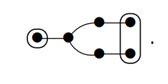
In the case \(d=2\), the Moufang quadrangles have Tits index \(\mathsf{^2D_{5,2}^{(2)}}\), with notation as in [30], which pictorially looks like
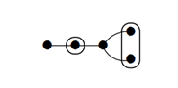
Hence, the dimensions of the varieties \(\mathcal{V}_1\) and \(\mathcal{V}_2\) related to this Moufang quadrangle are the numbers \(\frac12j(4m-3j-1)\) for \(m=5\) and \(j=2\) and \(4\), respectively, which is \(13\) and \(14\), respectively, which is \(5+4d\) and \(4+5d\), respectively, for \(d=2\). Of course, this can also be calculated from the dimensions of the root groups, which are \(2+d=4\) and \(1+2d=5\). All of this also shows \(t(1)=1\) and \(t(2)=4\).
It is shown in [15] that no domestic collineation, and hence no uniclass automorphism, exists for the case \(d=1\). The associated Weyl substructure would have to be a Moufang quadrangle of dimension \(9\) (both point and line space); hence the root groups would have to have dimension 3. However, no such Moufang quadrangle is known. This provides an alternative proof. Likewise, for the case \(d=8\), we would have a Moufang quadrangle with \(\mathop{\mathrm{\mathsf{dim}}}\mathcal{V}_1=37\) and \(\mathop{\mathrm{\mathsf{dim}}}\mathcal{V}_2=44\), implying that the root groups have dimensions \(10\) and \(17\). Also such a Moufang quadrangle does not exist; the closest come the exceptional Moufang quadrangle of type \(\mathsf{E_7}\), who has root group dimensions \(8\) and \(17\). Since \(8<10\), it is conceivable, and we conjecture, that there is a group of automorphisms of \(\mathsf{F_4}(\mathbb{F},\mathbb{F}^{(8)})\), with \(\mathbb{F}^{(8)}\) a Cayley division algebra over \(\mathbb{F}\) fixing an exceptional Moufang quadrangle of type \(\mathsf{E_7}\). However, no such automorphism is uniclass or domestic. But it would still be interesting to know whether such inclusion exists.
Simple Weyl substructures in generalised polygons
The last two rows of Table 3 are devoted to describing the dimensions of putative ovoids and ovoid-spread pairings in generalised polygons. There are only a few cases in which there is indeed a field around. We mention the quadrangles, where certainly also some non-Moufang quadrangles admit uniclass automorphisms with fixed point set an ovoid or an ovoid-spread pairing (for instance some finite non-classical quadrangles of order \(s\) admit polarities, see [25, Theorem 12.5.2]). In these cases, the dimensions must be read as degrees of freedom, where, in the finite case, single degrees correspond to \(s\) or \(s+1\), or \(t\) or \(t+1\) choices, with \(s+1\) the number of points on a line and \(t+1\) the number of lines through a point.
One notes that ovoid-spread pairings have exactly half of the dimension of the complete variety of point-line flags. Again this is explained by the fact that, in the Moufang case, such a polarity is the “mixed” analogue of Galois descent. Such polarities are known for generalised quadrangles (the so-called Suzuki quadrangles, see [35, §3.4.6]) and for the Moufang hexagons (split Cayley hexagons in characteristic \(3\) over a perfect field, or certain hexagons of mixed type, see [35, §7.7]). The uniclass automorphisms of Moufang hexagons are classified in [20], and besides the mentioned polarities, there are no more cases where an ovoid, spread or ovoid-spread pairing is fixed, except for one conjugacy class fixing an ovoid in the dual split Cayley hexagons over a field \(\mathbb{K}\) with characteristic different from \(3\) admitting no non-trivial cubic roots of the identity.
For other values of \(m\), very little is known. We do know, for instance, that no Moufang octagon admits a polarity. But it is not known in general whether there exist uniclass collineations of Moufang octagons fixing ovoids or spreads. For other values of \(m\), there exist self polar examples constructed freely. For instance, the ordinary free construction of a generalised \(2m\)-gon starting from an ordinary \((2m+1)\)-gon yields a self-polar generalised \(2m\)-gon. For more background on this free construction process, see [33].
Concerning notation, we note that in the second column, we have put the algebraic structure between parentheses behind the Coxeter symbol of the diagram, where the “gonality” of the rank 2 building appears in the superscript. The symbol in the first column has the gonality between parentheses, and not as superscript because of our general rule that the superscript indicates the place of the encircled nodes.
Observation 5.1 implies that all varieties of the Weyl substructures have a large dimension, at least half of the dimension of the corresponding variety of the ambient buildings. But this is not a sufficient condition. Indeed, Galois descent with a Galois group of order \(2\) provides many counter examples. Another prominent one is the following. Consider the metasymplectic space \(\mathsf{F_{4,1}}(\mathbb{K},\mathbb{A})\), with \(\mathbb{A}\) a separable quadratic division algebra, and select a subalgebra \(\mathbb{B}\) fixed under a non-trivial automorphism \(\sigma\) of \(\mathbb{A}\). Then \(\sigma\) can be extended to the whole metasymplectic space \(\mathsf{F_{4,1}}(\mathbb{K},\mathbb{A})\) and yields a non-trivial automorphism pointwise fixing a subspace isomorphic to \(\mathsf{F_{4,1}}(\mathbb{K},\mathbb{B})\). Typically, one can construct such automorphisms for \(\mathop{\mathrm{\mathsf{dim}}}_{\mathbb{K}}\mathbb{A}=2\mathop{\mathrm{\mathsf{dim}}}_{\mathbb{K}}\mathbb{B}\). Then for corresponding varieties \(\mathcal{V}_j(\mathbb{A})\) and \(\mathcal{V}_j(\mathbb{B})\) holds, with obvious notation that \[2\mathop{\mathrm{\mathsf{dim}}}\mathcal{V}_j(\mathbb{B})-\mathop{\mathrm{\mathsf{dim}}}\mathcal{V}_j(\mathbb{A})\in\{6,9,11\}, \mbox{ for all }j\in\{1,2,3,4\}.\]
These examples are domestic for \(\mathbb{A}\) associative, but none is uniclass as they fix chambers and act type-preserving while opposition on types is trivial.
However, in the opposite direction, Observation 5.1 explains why certain other automorphisms are not uniclass. We provide three simple examples.
Example 5.2. Line spreads in \(3\)-dimensional spaces are simple Weyl substructures. One could ask why elementwise stabilisers of plane spreads in \(5\)-dimensional projective spaces are not uniclass. We simply calculate its dimension over the ground field of the projective space, which is \(3\), whereas the dimension of the Grassmann variety of planes in a \(5\)-space is \(9\). Clearly \(2\cdot3<9\). Similar results hold for all other simple spreads.
Example 5.3. Since spreads of maximal singular subspaces of a polar space have the same dimension as an ovoid, one would expect elementwise stabilisers of a spread also to be uniclass. However, besides the fact that, if a collineation fixed elementwise a spread, then it would be point-domestic and hence by [21, Proposition 3.1] it would also stabilise lines, we calculate the dimension of the corresponding varieties and obtain, with the notation of the third row of Table 3, \[\begin{cases}
\mbox{Dimension spread}=\ell+k(m-1),\\
\mbox{Dimension variety of maximal singular subspaces}=m\ell+\frac12m(m-1)k,\\
\end{cases}\] which implies clearly that for \(m\geq 4\), the dimension of the spread is less than half the dimension of the variety of maximal singular subspaces. For \(m=3\), this is only the case when \(k<\ell\). For \(k\geq \ell\), a spread of a polar space of rank 3 satisfies the necessary condition of Observation 5.1 to be a Weyl substructure (but it is not, of course).
Likewise, for type \(\mathsf{D}_n\), one only obtains at least half the dimension (and then exactly half of the dimension) when \(d=4\), but that was expected since by triality, this is equivalent to fixing an ovoid. (However, note that in this case the collineation has class 2 and so, if one want to have as fixed structure just a spread, then we need an automorphism not preserving types.)
Example 5.4. Finally we consider the split Cayley hexagon as a substructure of the polar space \(\Gamma\) of type \(\mathsf{D_4}\), viewed as the fix structure of a triality, and we calculate again the relevant dimensions. Clearly the dimensions of the point space and the line space of the hexagon are both equal to \(5\). Now the dimension of the line space of \(\Gamma\) is \(9\), whereas the dimension of the flag space of type \(\{1,3,4\}\) is equal to \(6+3+2=11\). Hence the dimension of the point variety of the hexagon is less than half the dimension of the corresponding flag variety of \(\Gamma\), whereas the dimension of the line variety of the hexagon is more than half of the dimension of the line variety of \(\Gamma\).
Funding
Daan Rijpert is supported by Ghent University Special Research Fund, grant BOF.24Y. 2021.0029.01. and Hendrik Van Maldeghem is partially supported by Senior Fundamental Research Project G023121N of the Fund for Scientific Research—Flanders.
