The triplication method for constructing strong starters

1. Introduction

1.1. Background and motivation

The theoretical impetus for this study is Horton’s conjecture on the existence of strong starters. To make this Introduction independent of the main part of the paper, we recall the basic definitions.

A starter \(S\) in an additive abelian group \(G\) of order \(n=2k+1\geq 3\) is a set of \(k\) pairs \(\{\{x_i,\ y_i\}\}_{i=1}^k\) that partitions the set \(G^*=G\setminus \{0\}\), such that \(\{\pm(x_i-y_i)\mid \{x_i,\ y_i\}\in S\}= G^*\).

If all sums \(x_i + y_i\) for the pairs \(\{x_i, y_i\}\in S\) are distinct and nonzero modulo \(n\), then the starter \(S\) is called strong.

Starters are useful in the construction of various types of combinatorial designs, such as the one-factorization of complete graphs and round-robin tournaments. Strong starters, introduced in 1968 by Stanton and Mullin [12] to construct Room squares, have become used in constructing many other designs: Room cubes, Kotzig factorizations, Howell designs, Kirkman triple systems, Kirkman squares and cubes. (See [2] and the references therein).

For any \(G\) of odd order \(\geq 3\), the set of pairs \(\{\{x,\ -x\}\mid x\in G^*\}\) forms a starter in \(G\) called the canonical or patterned starter. The existence of strong starters is a much trickier problem. Based on theoretical results obtained between 1968 and 1989 and computations by Dinitz and Stinson [3], Horton [6] proposed the conjecture:

Conjecture 1.1 (Horton, 1989). All non-trivial finite abelian groups of odd order, except \(\mathbb{Z}_3\), \(\mathbb{Z}_5\), \(\mathbb{Z}_9\) and \(\mathbb{Z}_3\oplus \mathbb{Z}_3\), admit a strong starter.

We will be concerned with cyclic groups \(\mathbb{Z}_n\). The version of the above Conjecture restricted to this case was articulated much earlier [4, p. 170]. The results cited in [6] cover all admissible \(n\leq 999\), as well as all \(n\) such that \(3\nmid n\).

All known existence proofs (besides computational results for particular orders) use explicit algebraic constructions, either immediate (e.g. for prime orders \(>5\)) or inductive. In the latter approach, strong starters in \(\mathbb{Z}_\ell\) and in \(\mathbb{Z}_m\) are taken and a strong starter in \(\mathbb{Z}_{\ell m}\), where \(3\nmid \ell m\), is exhibited. The excepted case \(\ell = 5\) (quintuplication) is treated in [5]. No analytical triplication (\(\ell = 3\)) is known. The existence of strong starters in \(\mathbb{Z}_n\) of arbitrarily large orders divisible by 3 remains an open problem [13].

Oleg Ogandzhanyants, the first author, in his PhD thesis defended at Memorial University in 2025, addressed the problem of constructing strong starters of orders \(3m\) from strong starters of order \(m\) (triplicating) by introducing a triplication table as an intermediate combinatorial structure defined explicitly by the given strong starter of order \(m\). The triplication problem had thus been reduced to solving a modular Sudoku problem. Although this approach has not as of yet led to the settlement of Horton’s conjecture in the case of cyclic groups, its viability for practical construction of strong starters of orders \(3m\) has been demonstrated and some theory around the triplication process has emerged.

1.2. Our previous work and outline of this paper

This paper is a sequel to our previous work [11], which will be referred to frequently.

The triplication method aims to construct a strong starter in \(G = \mathbb{Z}_n\) of order divisible by 3, \(n = 3m\). In [11] we described triplication as a multi-part process. First, one constructs a triplication table (TT) given a strong starter of order \(m\) not divisible by 3. Then one sets up a Modular Sudoku Problem (MSP), which is a system of certain arithmetical equations and inequalities. These stages are fully formalized and readily programmed in a computer. Next, one must solve the resulting MSP. This is the most computationally demanding part of the process. While small cases can be attempted manually, we generally rely on a third-party SAT/SMT solver, z3 [8]. The final part, short and simple, serves to recover the final result (a strong starter of order \(n\)) from the original TT and the found solution of MSP by means of the Chinese Remainder Theorem (CRT).

This paper offers a broader look at triplication, with arithmetic, conceptual, and constructive advances, supporting examples and empirical observations.

An important limitation of the triplication method as given in [11] was the requirement that \(m\) be not divisible by 3. Here we remove this limitation (the arithmetic advance).

The conceptual advances include, first, an extended definition of the TT in Section 2, and second, a more general and flexible framework in Section 3 to set up an MSP and construct a strong starter of order \(3m\) based on the given TT and a contingent solution of the MSP. Theorem 3.7 solidifies this framework, ensuring that a TT and a solution of the MSP yield a strong starter.

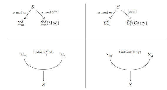
The general framework arose from an effort to unify two concrete scenarios of triplication shown in Figure 1 in the left and right columns respectively. We label them “Mod” and “Carry” and discuss their specifics in Sections 5 and 6. The top row in Figure 1 depicts analysis. We start with our objective, a strong starter \(S\) of order \(3m\), and work backward in order to identify properties of the objects corresponding to \(S\) involved in the triplication process: the TT \(\Sigma_m^S\) and a solution \(\tilde{\Sigma}_r^S\) of the MSP. Constraints described in Section 3.3 (necessary conditions of MSP’s solvability) are based on that analysis.

The bottom row depicts synthesis — what triplication is designed for. More precisely, it shows the flow chart of the algorithm to build a strong starter from a triplication table. The horizontal arrow symbolizes solution of an MSP to get a suitable (“congruous”) \(\tilde{\Sigma}\)-table. Finally, the two tables are combined to obtain a strong starter.

Due to Theorem 3.9, the sets of strong starters obtainable from the same triplication table in the two scenarios Mod and Carry are the same.

The constructive advances significantly extend an explicit construction of TT given in [11]. In Section 4.1, we introduce the notions of a triplication template and an admissible key that together give rise to a valid TT. In further subsections of Section 4, we analyze constructions that employ specific triplication templates based either on one starter of order \(m\) (like in [11] — but with nontrivial novelties in the case of a non-strong starter) or on three starters or on a starter and two algebraically constructed pseudostarters.

Constructive details of the Mod and Carry scenarios are elaborated upon in Sections 5 and 6, with examples.

Let \(m = 3^{\nu}p\), where \(p\) is odd and not divisible by 3. In Section 5.1 we assume that \(\nu = 0\) and recall the details of our approach as presented in [11]. In Section 5.2 we show how to set up a Sudoku-type problem modulo \(r = 3^{\nu +1}\), \(\nu \geq 1\), whose solution yields a strong starter of order \(3m\). This variant of triplication uses an extension of CRT where the moduli are not coprime (Appendix 2). The content of Section 5 was developed in part in the PhD thesis of OO but not reflected in our previous joint publication [11].

From a computational perspective, in a naive approach, solving a Sudoku problem modulo 9, 27, etc. is significantly more costly than solving one modulo 3. Furthermore, the necessity to use an extended CRT appears to be an undesirable complication. Although both of these apparent difficulties proved minor in the end, they prompted a search for alternatives.

It is possible to modify the method in such a way as to obtain an MSP modulo 3 regardless whether 3 is coprime with \(m\) or not. This is the content of Section 6. A crucial novelty lies in the simplest final step: instead of using CRT, we recover numbers from their quotients and remainders of division by \(m\) in a straightforward way.

In the proposed scheme, under any scenario the construction of a strong starter is contingent on solving an MSP. In Section 7, we discuss the MSP solvability and give more examples of strong starters constructed by our method. In Section 7.2 we put forward a conjecture regarding the MSP solvability, extending our conjecture in [11] to include all constructions of TTs described in Section 4. In Section 7.3, we discuss more general TTs found numerically.

Overall, our exposition here does not stress numerical work. However, all the presented theoretical schemes have been implemented in Python and extensively tested. A code for the Carry scenario is presented in Appendix 3. The results included in order to illustrate theory constitute a small fraction of all that have been computed. Some details of computations, less systematic than in Section 8 of [11] for reasons explained, are given in Appendix 4.

The paper concludes with a brief summary (Section 8).

It is important in this work to thoroughly distinguish between the notions of set, multiset, and tuple. Particularly important when working with starters is the notion of pairing (a set or a tuple of pairs). In Appendix 1 we review the definitions applicable in our context.

2. The triplication table

2.1. Definition of the triplication table \(\Sigma_m\)

Let \(n = 2k + 1\geq 3\) be an odd integer. Let \(S = \{\{x_i,y_i\} \mid i = 1,\ldots ,k\}\) be a strong starter in \(\mathbb{Z}_{n} = \{0,1,\ldots ,n – 1\}\). This means that the (unordered) pairing \(S\) has the following properties:

(i) The pairs of \(S\) form a partition of \(\mathbb{Z}_{n}^{*} = \mathbb{Z}_{n}\setminus \{0\}\).

(ii) The set of differences \(\{\pm (x_{i} – y_{i})\}_{i = 1}^{k}\) is exactly \(\mathbb{Z}_{n}^{*}\).

(iii) Each pair of \(S\) makes a unique nonzero sum modulo \(n\): if \(\operatorname {Sums}(S) = \{x_{i}+y_{i}|\{x_{i},y_{i}\} \in S\}\) then \(\operatorname {Sums}(S)\subset \mathbb{Z}_{n}^{*}\) and \(|\operatorname {Sums}(S)| = k\). (In (ii) and (iii), addition and subtraction of elements in \(\mathbb{Z}_{n}\) are performed modulo \(n\).)

Suppose now that \(n = 3m\). Let us explore the left arrow in the scheme Figure 1, top row (either column).

Consider the multiset \(S_{m}\) of pairs of \(S\) reduced modulo \(m\). Each of the properties of \(S\) implies the corresponding property of \(S_{m}\).

Denote by \(\mathfrak{w}S_{m}\) the multiset union of the elements of all pairs of \(S_{m}\).

Theorem 2.1. Let \(S\) be a strong starter in \(\mathbb{Z}_{3m}\), \(m = 2q + 1\), \(q \geq 1\). Let \[S_{m} = \{\{x \mod m, y \mod m\} \mid \{x, y\} \in S\}\]. Then (i) for \(x \in \mathbb{Z}_{m}\), the multiplicity of \(x\) in \(\mathfrak{w}S_{m}\) equals 3 if \(x \neq 0\) and 2 if \(x = 0\); (ii) \(S_{m}\) contains exactly one pair of the form \(\{t, t\}\), \(t \in \mathbb{Z}_{m}^{*}\), and for every \(d = 1, \ldots , q\) there are exactly three pairs whose difference are \(\pm d\) (mod \(m\)); (iii) at most three pairs in \(S_{m}\) yield the same nonzero sum modulo \(m\) and at most two pairs in \(S_{m}\) yield a sum of zero modulo \(m\); (iv) No two pairs in \(S_{m}\) are identical.

Proof. (i) Since the elements of \(\mathbb{Z}_{3m}^{*}\) reduced modulo \(m\) form a multiset containing exactly three copies of each element of \(\mathbb{Z}_{m}^{*}\) and exactly two \(0\)’s, the same distribution of elements appears in \(\mathfrak{w}S_{m}\). (ii) follows from property (ii) of the strong starter \(S\). Here \(t \neq 0\) because neither of the pairs \(\{m, m\}\), \(\{2m, 2m\}\), \(\{m, 2m\}\) belongs to the strong starter \(S\). (iii) follows from property (iii) of the strong starter \(S\). (iv) The proof is an adaptation of end of proof of Theorem 7.2 in [11]. Suppose there are pairs \(\{x, y\}\) and \(\{x’, y’\}\) in \(S\) such that \(x \mod m = x’ \mod m = u\) and \(y \mod m = y’ \mod m = v\). We have \(x = mU + u\), \(y = mV + v\), \(x’ = mU’ + u\), \(y’ = mV’ + v\) for some \(U,V,U’,V’\in \{0,1,2\}\). By property (ii) of a strong starter, \(x – y\not\equiv x’ – y’\) (mod \(3m\)), hence \(U – V\not\equiv U’ – V’\) (mod 3). By property (iii) of a strong starter, \(x + y\not\equiv x’ + y’\) (mod \(3m\)), hence \(U + V\not\equiv U’ + V’\) (mod 3). Therefore \(U – U’\not\equiv \pm (V – V’)\) (mod 3). Since the only nonzero residues modulo 3 are \(\pm 1\), this implies \(U – U’\equiv 0\) (mod 3) or \(V – V’\equiv 0\) (mod 3). In either case we obtain a contradiction with property (i) of a strong starter. For instance, if \(U – U’\equiv 0\) (mod 3), then \(x – x’ = m(U – U’)\equiv 0\) (mod \(3m\)), so \(x\equiv x’\) (mod \(3m\)), a contradiction. \(\square\)

Definition 2.2. A triplication table of order \(m = 2q + 1\) is a pairing \(\Sigma_m = [(u_0,v_0),(u_1,v_1), \ldots ,(u_{3q},v_{3q})]\) with components in \(\mathbb{Z}_{m}\) satisfying the properties (i) an element \(x\in \mathbb{Z}_{m}\) is contained in \(\Sigma_m\) three times if \(x\neq 0\) and two times if \(x = 0\) (ii) \(\Sigma_m\) contains exactly one pair of the form \((t,t)\), namely \(u_0 = v_0 = t\) with \(t\neq 0\). For every \(d = 1,\ldots ,q\), there are exactly three pairs with directed difference \(\hat{d}\) modulo \(m\) namely \[v_{3d – 2} – u_{3d – 2} = v_{3d – 1} – u_{3d – 1} = v_{3d} – u_{3d} = \hat{d},\tag{1}\] where \(\hat{d}\) is either \(d\) or \(- d\), and it must be the same for all 3 such pairs. (iii) For \(s\in \mathbb{Z}_{m}\), there are at most three pairs in \(\Sigma_m\) that make the sum \(s\) modulo \(m\) if \(s\neq 0\), and at most two such pairs if \(s = 0\). (iv) No two pairs in \(\Sigma_m\) are identical.

Given an ordered pair \((u,v)\), we define the directed difference as \(v-u\).

The conditions in Definition 2.2 essentially mirror the properties of the modulo-\(m\) reduced starter \(S\) from Theorem 2.1, but with the pairs ordered in a specific way.

While \(\Sigma_m\) is mathematically defined as an ordered pairing, it is convenient to display it as a table using the layout introduced in [11], governed by the following rules. The table contains \(q + 1\) rows and 3 columns. The rows are indexed by \(0,1,\ldots ,q\) the columns are indexed by \(0,1,2\) The top row, called also the special row, is incomplete. It contains a single pair of type \((t, t)\), \(t\in \mathbb{Z}_{m}^{*}\). By convention, we place this pair in column 1 (central). The value \(t\) is called the key (of the table). The rows indexed 1 to \(q\) are called regular. The \(i\)-th row (for \(i = 1,\ldots ,q\)) contains pairs whose directed differences have common value \(\pm i\), cf. (1). The regular part of the triplication table consists of the \(3q\) pairs in the \(q\) regular rows.

Definition 2.3. Let \(S\) be a strong starter in \(\mathbb{Z}_{3m}\) and let \(S_{m}\) be its reduction modulo \(m\) as in Theorem 2.1. Suppose the pairs in \(S_{m}\) and elements in the pairs are ordered so as to satisfy the conditions \(v_{0} – u_{0} = 0\) and (1). The obtained pairing is a triplication table denoted \(\Sigma_{m}^{S}\). We say that \(\Sigma_{m}^{S}\) is induced by \(S\).

There is a preferred order where \(\hat d=d\) for \(d=1,\ldots,q\), but in general we allow different signs of each \(\hat d\) for compatibility with [11].

Remark 2.4. Theorem 2.1 guarantees that the ordering required in Definition 2.3 is always possible and the obtained pairing satisfies the requirements of Definition 2.2. However there is a certain freedom in pair ordering. Indeed, while the row index for every pair is fixed by Eq. (1) (the unique pair \((t,t)\) is placed in the special row), the column index of the pair is not specified. So there are \(3! = 6\) possibilities to arrange pairs within every row, thus a total of \(6^{q}\) possible arrangements for \(\Sigma_{m}^{S}\). Also, there are \(2^{q}\) choices of signs for the directed differences \(\hat{d}\).

In view of the latter Remark, we introduce an equivalence relation on the set of triplication tables.

Definition 2.5. Two TTs of the same order are equivalent if one can be obtained from the other by (i) some permutation of pairs (necessarily within the same row) and (ii) simultaneously reversing the order of components in all 3 pairs in certain rows.

We denote the equivalence class of a given triplication table \(\Sigma_{m}\) by \([\Sigma_{m}]\).

Returning to Definition 2.3 and Remark 2.4, we observe that to every strong starter \(S\) in \(\mathbb{Z}_{3m}\) there corresponds a unique equivalence class \([\Sigma_{m}^{S}]\) of TTs.

Remark 2.6. If \(S\) and \(Q\) are two strong starters of order \(3m\), the equality \([\Sigma_{m}^{S}] = [\Sigma_{m}^{Q}]\) does not imply \(S = Q\). In general, the correspondence \(S \leftrightarrow [\Sigma_{m}^{S}]\) is of the type many-to-one.

An approach to building a TT has been proposed in [11]; it will be further developed and generalized in Section 4. Constructions to be described involve special columnar arrangements of pairs in TTs, not shared by different tables of the same equivalent class. Some terminology related to columnar arrangements will be helpful in the sequel.

Definition 2.7. A pseudostarter in \(\mathbb{Z}_{m}\), \(m = 2q + 1\), is a pairing \(\{\{x_{i},y_{i}\}, i = 1,\ldots ,q\}\) such that \(x_{i},y_{i}\in \mathbb{Z}_{m}\) and the differences \(\pm (y_{i} – x_{i})\) (mod \(m\)) comprise \(\mathbb{Z}_{m}^{*}\). An ordered pseudostarter is a pairing \([(x_{1},y_{1}),\ldots ,(x_{q},y_{q})]\) where \(y_{i} – x_{i}\equiv \pm i\) (mod \(m\)), \(i = 1,\ldots ,q\).

Every starter is a pseudostarter, but the converse is not true. In a pseudostarter, it is not required that the pairs \(\{x_{i},y_{i}\}\) form a partition of \(\mathbb{Z}_{m}^{*}\). Some elements may appear more than once, some may be missing, and the value 0 is permitted.

Definition 2.8. A triple of pseudostarters \(T_{1}\), \(T_{2}\), \(T_{3}\) in \(\mathbb{Z}_{m}\) is balanced if the multiset union \(T_{1} \uplus T_{2} \uplus T_{3}\) contains 0 exactly twice, one nonzero element once, and every other element of \(\mathbb{Z}_{m}^{*}\) exactly three times.

Proposition 2.9. The three columns of the regular part of a triplication table \(\Sigma_m\) form a balanced triple of pseudostarters in \(\mathbb{Z}_{m}\).

Proof. The statement follows from comparison of Definitions 2.2, 2.7, and 2.8. The key value \(t\) is contained twice in the special row. By item (i) of Definition 2.2, it must occur exactly once in the regular part of the table. \(\square\)

2.2. Objects associated with a triplication table \(\Sigma_m\)

Let us introduce some notation and auxiliary objects associated with \(\Sigma_m\). In the sequel we label the pairs and their entries in \(\Sigma_m\) as follows: the pair in the special 0-th row is \((u_0,v_0)\) (so \(u_0 = v_0 = t\)); the pairs in a regular \(k\)-th row ( \(k = 1,\ldots ,q\)) are: \((u_{3k – 2},v_{3k – 2})\), \((u_{3k – 1},v_{3k – 1})\), \((u_{3k},v_{3k})\).

We will use two-index notation \(\langle i,\ell \rangle\) to indicate positions of the entries (components) in \(\Sigma_m\). Here \(i\in \{0,\ldots ,3q\}\) is the index of the pair containing the entry, and \(\ell \in \{0,1\}\) indicates the position within the pair: \(\ell = 0\) points to \(u_{i}\) and \(\ell = 1\) points to \(v_{i}\).

We treat residues modulo \(m\) as colors. A monochrome set is the set of positions of entries in the triplication table that share the same value (color).

Definition 2.10. The monochrome set \(M_{c}\) of color \(c\in \{0,\ldots ,m – 1\}\) is the set of double indices \(\langle i,\ell \rangle\) such that the corresponding entry of the table \(\Sigma_m\) has value \(c\).

Proposition 2.11. In a triplication table, the sizes of the monochrome sets satisfy: \(|M_{0}| = 2\) and \(|M_{c}| = 3\) if \(c\neq 0\).

Proof. This is due to item (i) of Definition 2.2. \(\square\)

For \(s\in \{0,\ldots ,m – 1\}\), denote by \(W_{s}\) the set of indices \(i\) of pairs \((u_{i},v_{i})\) in \(\Sigma_m\) such that \(u_{i} + v_{i}\equiv s\) (mod \(m\)).

Proposition 2.12. In a triplication table, the sizes of sets \(W_{s}\) satisfy: \(|W_{0}|\leq 2\) and \(|W_{s}|\leq 3\) if \(s\neq 0\).

Proof. This is due to item (iii) of Definition 2.2. \(\square\)

Definition 2.13. The set \(W_{s}\) is called a weak set (with sum \(s\)) if either \(s = 0\) or \(|W_{s}| > 1\). For a weak set \(W_{s}\), the set \(W P_{s} = \{(u_{i},v_{i}) \mid i\in W_{s}\}\) is called a weak pair sets with sum \(s\). Pairs that are not weak are called strong. In other words, a pair is strong if its sum is unique and nonzero.

3. The modular Sudoku problem

This section is concerned with tables denoted \(\tilde{\Sigma}_{r}\) and \(\tilde{\Sigma}_{3}\) in Figure 1.

3.1. Discriminating 3-to-1 modular reduction \(\mathbb{Z}_{3m} \to \mathbb{Z}_{m}\)

The map \(x\mapsto x\bmod m\), \(\mathbb{Z}_{3m}\to\mathbb{Z}_{m}\), is 3-to-1. Hence, knowing \(u = x\) (mod \(m\)), in order to recover \(x\in \mathbb{Z}_{3m}\), we need a way to make a choice between 3 candidate values of \(x\). This can be done uniquely if, for every \(x\in \mathbb{Z}_{3m}\), we associate not just \(u\) but a pair \((u,U)\) where \(u = x\) (mod \(m\)) and \(U\) is a discriminator — a numerical parameter that takes different values for \(x = u\), \(x = u + m\), and \(x = u + 2m\).

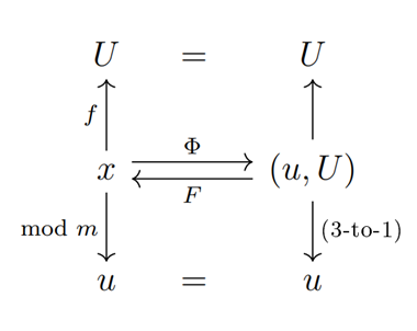
Let us encode a number \(x\in \mathbb{Z}_{3m}\) by a pair \((u,U)\in \mathbb{Z}_{m}\times \mathcal{Z}\), where \[u = x\mod m\text{ and }U = f(x)\tag{2}\], \(\mathcal{Z}\) is a finite set of cardinality \(\geq 3\). Here, \(f:\mathbb{Z}_{3m}\to \mathcal{Z}\) is the discriminating function, such that the map \(\Phi :x\mapsto (u,U)\) is one-to-one.

Let \(\Omega \subset \mathbb{Z}_{m}\times \mathcal{Z}\) be the range of the map \(\Phi\). Since \(\Phi\) is one-to-one, there exists the inverse (decoding) map \(F:\Omega \to \mathbb{Z}_{3m}\), which recovers \(x\) given \((u,U)\).

This abstract scheme, visualized in Figure 2, will be called a discrimination scenario (or just “scenario” for short).

For reference, let us summarize the discriminating property of the correspondence \(x\leftrightarrow(u,U)\) in a formal proposition, which is in fact a tautology.

Proposition 3.1. Let \(x,y\in \mathbb{Z}_{3m}\) and \(\Phi (x) = (u,U)\), \(\Phi (y) = (u,V)\), where \(\Phi :\mathbb{Z}_{3m}\to \mathbb{Z}_{m}\times \mathcal{Z}\) is one-to-one. Then \(x\neq y\) iff \(U\neq V\).

In practice, we will use two particular scenarios, which we label “Mod” and “Carry”, and we subscript the functions \(f\), \(\Phi\), and \(F\) accordingly.

Mod scenario: assuming \(m = 3^{\nu}p\), \(\nu \geq 0\), and \(3\nmid p\), \[f_{\mathrm{Mod}}(x) = x\mod 3^{\nu +1}.\tag{3})\] Here \(\mathcal{Z} = \mathbb{Z}_{3^{\nu +1}}\), \(\Omega = \{(u,U)\in \mathbb{Z}_{m}\times \mathcal{Z}:U\in \{u,u + 3^{\nu},u + 2\cdot 3^{\nu}\}\}\) (with addition modulo \(3^{\nu +1}\)).

Carry scenario: regardless of whether \(m\) is divisible by 3, \[f_{\mathrm{Carry}}(x) = \lfloor x / m\rfloor.\tag{4}\] Here \(\mathcal{Z} = \mathbb{Z}_{3}\) and \(\Omega = \mathbb{Z}_{m}\times \mathcal{Z}\).

In either scenario, given \(x\in \mathbb{Z}_{3m}\), the pair \((u,U)\) (2) is found by one of the formulas (3) or (4). Further details, in particular, the inverse maps \(F:(u,U)\to x\), are treated in Sections 5 and 6 (where the nickname “Carry” is clarified), respectively.

Example 3.2. Table 1 illustrates discrimination in the Mod scenario. It displays, for each \(u\in \mathbb{Z}_{m}\), the corresponding values of \(x\in \mathbb{Z}_{3m}\) and the discriminators \(U = f_{\mathrm{Mod}}(x)\), see Eq. (3), in the cases \(m = 7 = 3^{0}\cdot 7\) (left) and \(m = 15 = 3^{1}\cdot 5\) (right). In the Carry scenario, each cell in the “\(U\)” column of both tables, calculated according to Eq. (4), would consist of values 0, 1, 2 in that order.

Table 1. Correspondences \(x\leftrightarrow (u,U)\) in Mod scenario for \(m = 7\) (left) and \(m = 15\) (right)

\(u\)	\(x\in\mathbb{Z}_{21}\)	\(U\)
0	0, 7, 14	0, 1, 2
1	1, 8, 15	1, 2, 0
2	2, 9, 16	2, 0, 1
3	3, 10, 17	0, 1, 2
4	4, 11, 18	1, 2, 0
5	5, 12, 19	2, 0, 1
6	6, 13, 20	0, 1, 2

\(u\)	\(x\in\mathbb{Z}_{45}\)	\(U\)
0	0, 15, 30	0, 6, 3
1	1, 16, 31	1, 7, 4
2	2, 17, 32	2, 8, 5
3	3, 18, 33	3, 0, 6
4	4, 19, 34	4, 1, 7
…	…	…
14	14, 29, 44	5, 2, 8

3.2. “Arithmetic” on discriminators

In the general setting described in Section 3.1 let us introduce symbolic notation for “difference” \(V\boxminus U\) and “sum” \(U\boxplus V\) in \(\mathcal{Z}\) induced from the difference and sum of two elements in \(\mathbb{Z}_{3m}\) as follows: \(f(y)\boxminus f(x) = f(y – x), \qquad f(x)\boxplus f(y) = f(x + y),\) where \(+\) and \(-\) in the right-hand sides are the usual arithmetic operations modulo \(3m\). Suppose \((u,U)\) and \((v,V)\) are in \(\Omega\). The above equations can be written as \[V\boxminus U = f(F(v,V) – F(u,U)), \quad U\boxplus V = f(F(u,U) + F(v,V)).\tag{5}\] The right-hand sides depend also on \(u\) and \(v\). Hence the formulas (5) do not, in general, define two-argument functions from a Cartesian square of a certain set (say, \(\mathcal{Z}\)) into itself. This is why we put the word “arithmetic” in the heading of this subsection in quotation marks. Informally speaking, we want the left-hand sides in (5) to be understood just as abbreviations of the right-hand sides. For a rigorous definition, we should use the symbols \(\boxminus_{u,v}\), \(\boxplus_{u,v}\) in the left sides of (5) to define a family of two-argument partial functions parametrized by pairs \((u,v)\in \mathbb{Z}_{m}\times \mathbb{Z}_{m}\). The admissible pairs \((U,V)\) for every such function are those for which \((u,U)\in \Omega\) and \((v,V)\in \Omega\).

Returning to the indexless notation, every time the “operations” \(\boxplus\) and \(\boxminus\) are encountered, the values \(u\) and \(v\) are to be given (in general) along with \(U\) and \(V\). With this understanding, as we will see in the next subsection, the unencumbered notation will be very helpful.

In the Mod scenario, with \(U = f_{\mathrm{Mod}}(x)\), \(V = f_{\mathrm{Mod}}(y)\), formulas (5) become \[V\boxminus U = (V – U)\mod 3^{\nu +1}\text{ and }U\boxplus V = (U + V)\mod 3^{\nu +1}. \tag{6}\] They agree with usual arithmetic operations modulo \(3^{\nu +1}\). In this case \(\boxplus\) and \(\boxminus\) unambiguously represent the standard binary operations in \(\mathcal{Z} = \mathbb{Z}_{3^{\nu +1}}\).

In the Carry scenario, the situation is more complicated: in order to calculate \(V\boxminus U\) and \(U\boxplus V\) by (5) we must know their counterparts \(u\) and \(v\) in the pairs that belong to \(\Omega\). The explicit formulas are derived in Section 6, see Eq. (23).

The following proposition is an extension of Proposition 3.1. It will be used to discriminate the results of arithmetic operations modulo \(3m\) when the results modulo \(m\) coincide.

Proposition 3.3. Suppose, for \(i = 1,2\), \(x_{i},y_{i}\in \mathbb{Z}_{3m}\), \(\Phi (x_{i}) = (u_{i},U_{i})\), and \(\Phi (y_{i}) = (v_{i},V_{i})\). (a) Suppose that \(u_{1} + v_{1}\equiv u_{2} + v_{2}\) (mod \(m\)). Then \(x_{1} + y_{1}\neq x_{2} + y_{2}\) in \(\mathbb{Z}_{3m}\) iff \(U_{1}\boxplus V_{1}\neq U_{2}\boxplus V_{2}\) in \(\mathcal{Z}\). (b) Suppose that \(v_{1} – u_{1}\equiv v_{2} – u_{2}\) (mod \(m\)). Then \(y_{1} – x_{1}\neq y_{2} – x_{2}\) in \(\mathbb{Z}_{3m}\) iff \(V_{1}\boxminus U_{1}\neq V_{2}\boxminus U_{2}\) in \(\mathcal{Z}\).

Proof. (a) Introduce \(z_i=x_i+y_i\), \(w_i=u_i+v_i\), \(W_i=U_i\boxplus V_i\), for \(i=1,2\). The claim becomes: “Let \(w_1=w_2\). Then \(z_1\neq z_2\) iff \(W_1\neq W_2\).” Since \(\Phi(z_i)=(w_i,W_i)\) by (5), the claim is true by Proposition 3.1.

(b) We use the same argument as in (a) with \(z_i=y_i-x_i\), \(w_i=v_i-u_i\), \(W_i=V_i\boxminus U_i\), for \(i=1,2\). \(\square\)

3.3. A table \(\tilde{\Sigma}^{S}\) consisting of discriminating values

In Section 2.1 we explained the left arrow in the schemes shown in the top row of Fig 1 (in either column). Here we will similarly explain the right arrow and its target, the table \(\tilde{\Sigma}_{*}^{S}\).

Let \(S\) be a strong starter of order \(3m\), \(m = 2q + 1\). In an abstract discrimination scenario, along with the table \(\Sigma_{m}^{S} = \{(u_{i},v_{i})\}_{i = 0}^{3q}\), let us consider a table \(\tilde{\Sigma}^{S} = \{(U_{i},V_{i})\}_{i = 0}^{3q}\) of the same layout and filled with ordered pairs of elements of \(\mathcal{Z}\), the target set of the function \(f\) in (2).

Thus, the pairs \((U,V)\) of \(\tilde{\Sigma}^{S}\), obtained from the pairs \((x,y)\) of a strong starter \(S\), are aligned with the pairs \((u,v)\) of \(\Sigma_{m}^{S}\) in the following way (for \(0\leq i\leq 3q\)):

This fixed alignment makes the values \(V_i\boxminus U_i\), \(U_i\boxplus V_i\) unambiguously defined by Eqs. (5) with \(u=u_i\), \(v=v_i\).

Keeping the description still abstract, but having our two concrete scenarios in mind, we identify \(\mathcal{Z}\) with number set \(\mathbb{Z}_r=\{0,1,\ldots,r-1\}\). In the Mod scenario with \(m=3^\nu p\), \(3\nmid p\), we have \(r=3^{\nu+1}\), while in the Carry scenario \(r=3\) for any \(m\).

The additional condition, where \(0_a\) denotes zero element of \(\mathbb{Z}_a\),

will be henceforth assumed. It implies that \(\Phi(0_{3m})=(0_m,0_r)\) and \(F(0_m,0_r)=0_{3m}\). In particular, the condition (8) is fulfilled in the scenarios Mod and Carry.

As the set \(\mathcal{Z}\) is agreed upon, from now on we will write \(\tilde{\Sigma}_r^S\) instead of \(\tilde{\Sigma}^S\). By construction, the table \(\tilde{\Sigma}_r^S\) has the following properties, or, as we prefer to say, obeys the following constraints. (Double parentheses are used to distinguish between constraints and equation numbers in references.)

((0)) Range Constraints. Variables \(U_i,V_i\) take values in the set \(\{0,1,\ldots,r-1\}\).

((1)) Row Constraints. The “differences” \(D_i=V_i\boxminus U_i\) in each regular row of the table are distinct. The “difference” \(D_0=V_0\boxminus U_0\) is nonzero (i.e. \(D_0\in\{1,\ldots,r-1\}\)).

((2)) Weak Set Constraints.

Recall that weak sets associated with table \(\Sigma_m^S\) are defined in Definition 2.13.

For every weak set \(W_s\):

(a) In the case \(s\neq 0\), the “sums” \(\{U_i\boxplus V_i,\ i\in W_s\}\) are distinct.

(b) In the case \(s=0\), the “sums” \(\{U_i\boxplus V_i,\ i\in W_0\}\) are distinct and nonzero.

((3)) Color Constraints.

Recall that monochrome sets \(M_c\) associated with table \(\Sigma_m^S\) are defined in Definition 2.10.

(a) In the case \(c\neq 0\), the values of \(U_i\) or \(V_i\) at the positions corresponding to the double indices \(\langle i,\ell\rangle\in M_c\) are distinct.

(b) In the case \(c=0\), the values of \(U_i\) or \(V_i\) at the positions corresponding to the double indices \(\langle i,\ell\rangle\in M_c\) are distinct and nonzero.

((4)) Consistency Constraints. The pairs \((u_i,U_i)\) and \((v_i,V_i)\) lie in the range \(\Omega\) of the map \(\Phi\) defining the discrimination scenario currently in use.

The constraints ((0))–((3)) directly correspond to the constraints 1–4 in [11, Sec. 6], where, in our present terminology, the Mod scenario was used in the case \(\nu=0\) (i.e. \(m\) coprime with 3). In that case, the constraints ((4)) are vacuous. They will also be vacuous in the Carry scenario.

In the Mod scenario with \(\nu>0\) the constraints ((4)) take the form of Modular Compatibility Conditions: \(U_i\equiv u_i\pmod{3^\nu}\) and \(V_i\equiv v_i\pmod{3^\nu}\) for \(i\in\{0,1,\ldots,3q\}\), cf. the description of the set \(\Omega\) next to Eq. (3).

Since the map \(\Phi\) is invertible, and due to the Consistency Constraints, the strong starter \(S\) used to construct the tables \(\Sigma_m^S\) and \(\tilde{\Sigma}_r^S\) can be uniquely recovered from these two tables: \(x_i=F(u_i,U_i)\), \(y_i=F(v_i,V_i)\), \(i\in\{0,1,\ldots,3q\}\).

3.4. Congruous table, Modular Sudoku Problem, and the recovery of a strong starter

While the departure point of the preceding discussion was a strong starter \(S\) in \(\mathbb{Z}_{3m}\), the properties (constraints) ((0))–((4)) did not mention \(S\) explicitly; implicitly \(S\) was still present via the TT \(\Sigma_m^S\). Now we want to completely eliminate \(S\) from the picture. The new point of departure will be a triplication table per se, regardless of its origin.

Definition 3.4. Let the following be given: (i) a triplication table \(\Sigma_{m}\) of order \(m\), see Definition 2.2, (ii) a discrimination scenario defined by a set \(\mathcal{Z} = \mathbb{Z}_{r}\) and a function \(f:\mathbb{Z}_{3m}\to \mathcal{Z}\) such that the map \(\Phi :x\mapsto (u,U)\) defined by Eq. (2) is one-to-one. Let \(\{W_{s}\}\) and \(\{M_{c}\}\) be the collections of weak, resp., monochrome sets associated with \(\Sigma_{m}\) as defined in Section 2.2 and operations \(\boxplus\) \(\boxminus\) be defined by (5) in the chosen scenario. A table \(\tilde{\Sigma}_{r}\) satisfying the constraints ((0)) – ((4)) stated above is said to be congruous with TT \(\Sigma_{m}\) (in the given scenario). The following problem is called the Modular Sudoku Problem (related to \(\Sigma_{m}\) in the given scenario): Find a table \(\tilde{\Sigma}_{r}\) congruous with \(\Sigma_{m}\).

Definition 3.5. Suppose \(\Sigma_{m}\) is a TT of order \(m = 2q + 1\) and \(\tilde{\Sigma}_{r}\) is a table congruous with \(\Sigma_{m}\) in the given discrimination scenario with mutually inverse maps \(\Phi\) and \(F\). For aligned pairs \((u_{i},v_{i})\) of \(\Sigma_{m}\) and \((U_{i},V_{i})\) of \(\tilde{\Sigma}_{r}\) put \[x_{i} = F(u_{i},U_{i}),\quad y_{i} = F(v_{i},V_{i})\quad \text{ for } i = 0,\ldots ,3q.\tag{9}\] The right-hand sides are defined due to the Consistency Constraints. The so obtained pairing \([(x_{i},y_{i})]_{i = 0}^{3q}\) is said to be congruous with TT \(\Sigma_{m}\) in the given scenario. To add specificity, the pairing \([(x_{i},y_{i})]_{i = 0}^{3q}\) is said to be congruous with \(\Sigma_{m}\) via \(\tilde{\Sigma}_{r}\). Referring to Eqs. (9), we also say that \(\Sigma_{m}\) and \(\tilde{\Sigma}_{r}\) yield the pairing \(S\).

The analysis in Section 3.3 can be summarized in the following formal statement.

Proposition 3.6. Suppose \(S\) is a strong starter of order \(3m\), \(\Sigma_m^S\) is the triplication table induced by \(S\) (see Definition 2.3), and \(\tilde{\Sigma}_r^S\) is the table defined in Section 3.3 in the given discrimination scenario (with \(\mathcal{Z}=\mathbb{Z}_r\)). Then (i) the table \(\tilde{\Sigma}_r^S\) is congruous with \(\Sigma_m^S\); (ii) the original starter \(S\) is congruous with \(\Sigma_m^S\) via \(\tilde{\Sigma}_r^S\).

In this sense, the constraints ((0))–((4)) are necessary conditions for the tables \(\Sigma_m\) and \(\tilde{\Sigma}_r\) to yield a strong starter by means of Eqs. (9).

We do not claim that these conditions are sufficient for the existence of a \(\tilde{\Sigma}_r\) congruous with \(\Sigma_m\); in fact, they are not — see Section 7. But the next weaker statement already justifies the triplication idea.

Theorem 3.7. Let \(\Sigma_{m} = [(u_{i},v_{i})]_{i = 0}^{3q}\) be a triplication table of order \(m = 2q + 1\) (as described in Definition 2.2). Fix a discrimination scenario with set \(\mathcal{Z} = \mathbb{Z}_{r}\), \(r \geq 3\), and decoding function \(F\). Suppose \(\tilde{\Sigma}_{r}\) is a table congruous with \(\Sigma_{m}\) in the given scenario. Then the pairing \(S = [(x_{i},y_{i})]_{i = 0}^{3q}\) defined by Eqs. (9), that is, the unique pairing congruous with \(\Sigma_{m}\) via \(\tilde{\Sigma}_{r}\), is a strong starter in \(\mathbb{Z}_{3m}\).

Proof. We give a structural explanation dropping the indices of all variables for more transparency.

1. The pairing \(S\) contains \(3q+1\) pairs \((x,y)\) of integers \(x\) and \(y\). The components of each pair are found by \(x=F(u,U)\) and \(y=F(v,V)\), where \((u,v)\) is a pair from the TT \(\Sigma_m\), \((U,V)\) is the aligned pair from \(\tilde{\Sigma}_r\), and \(F\) is the decoding map inverse to \(\Phi\) (Figure 2). By Eqs. (9) and definition of \(F\), these \(6q+2=3m-1\) components of \(S\) are from \(\mathbb{Z}_{3m}\).

Let us show that they are all distinct and nonzero.

Distinct: Constraint ((3a)) guarantees that identical entries in \(\Sigma_m\) are aligned with distinct entries in \(\tilde{\Sigma}_r\). Then Proposition 3.1 implies that no two components in \(S\) are equal.

Nonzero: Constraint ((3b)) guarantees that entry \(0_m\) in \(\Sigma_m\) is aligned with nonzero entry in \(\tilde{\Sigma}_r\). Since \(F(0_m,0_r)=0_{3m}\) and \(F\) is one-to-one, \(S\) does not include 0 as a component.

Thus, \(S\) is a partition of \(\mathbb{Z}_{3m}^{*}\).

2. By Definition 2.2, all three differences \(v-u\) for pairs in each regular row of TT are equal. Constraint ((1)) guarantees that differences \(V\boxminus U\) for the correspondingly aligned three pairs from \(\tilde{\Sigma}_r\) are distinct. In addition, \(V_0\boxminus U_0\neq 0\) for the pair aligned with the pair \((t,t)\) from the special row of TT. Then Proposition 3.3(b) implies that all differences in \(S\) lie in \(\mathbb{Z}_{3m}^{*}\) and are distinct.

Finally, we prove by contradiction that \((y-x)\neq -(y’-x’)\) mod \(3m\). Indeed, if it were to happen that \((y-x)=-(y’-x’)\) mod \(3m\) for some pairs \((x,y),(x’,y’)\in S\), then, by (2), \((v-u)=-(v’-u’)\) mod \(m\).

If \((u,v)\) and \((u’,v’)\) are in the same row of TT, the clause concerning \(\hat d\) in Definition 2.2 (the line following Eq. (1)) implies that \((v-u)=(v’-u’)\) mod \(m\). But then \(2(v-u)=0\) mod \(m\), and this is impossible since \(2\nmid m\) and \(v-u\neq 0\) mod \(m\).

If \((u,v)\) and \((u’,v’)\) are in distinct rows of the TT, then \(v-u=d_1\), \(v’-u’=d_2\neq\pm d_1\). Again, \(d_1+d_2\equiv0\) mod \(m\) is impossible since \(|d_i|\leq q\) and \(m=2q+1\).

So \(S\) is a starter in \(\mathbb{Z}_{3m}\).

3. Constraint ((2)) guarantees that whenever two pairs from TT have the same sum \(u+v\), the sums \(U\boxplus V\) for the aligned two pairs from \(\tilde{\Sigma}_r\) are distinct. In addition, if \(u+v=0_m\) then for the aligned pair \(U\boxplus V\neq0_r\). Proposition 3.3(a) implies that the sums \(x+y\) of pairs in \(S\) are nonzero and distinct in \(\mathbb{Z}_{3m}\), so \(S\) is a strong starter in \(\mathbb{Z}_{3m}\). \(\square\)

We emphasize that the existence of a table \(\tilde{\Sigma}_r\) congruous with given TT \(\Sigma_m\) in the given scenario is not guaranteed. To find \(\tilde{\Sigma}_r\) amounts to solving an MSP and we offer no theoretical recipe for that.

3.5. Scenario-independence of the set of congruous starters

We mentioned two concrete discrimination scenarios, and there can conceivably be many more. The natural question arises: is any scenario better than others, either universally or for the particular given triplication table \(\Sigma_m\)? Let us understand “better” to mean “yielding more solutions”. In particular, can it happen that for the same \(\Sigma_m\) the Modular Sudoku Problem has no solution in one scenario but at least one solution in another?

The answer is: no. In all valid scenarios, the MSP and the recovery formulas (9) supply the same set of strong starters.

Notation 3.8. Fix \(m=2q+1\). Let \(\mathcal{A}\) be a discrimination scenario satisfying assumption (8). For the given triplication table \(\Sigma_m\), the set of (ordered) strong starters congruous with \(\Sigma_m\) in scenario \(\mathcal{A}\) is denoted \(\mathrm{ST}_{\mathcal{A}}(\Sigma_m)\).

Theorem 3.9. Fix \(m = 2q + 1\). Let \(\Sigma_{m}\) be a triplication table as defined in Section 2. Suppose \(\mathcal{A}\) and \(\mathcal{B}\) are two discrimination scenarios satisfying assumption (8). Then \(\mathrm{ST}_{\mathcal{A}}(\Sigma_{m}) = \mathrm{ST}_{\mathcal{B}}(\Sigma_{m})\).

Proof. The roles of \(\mathcal{A}\) and \(\mathcal{B}\) are symmetric, so it suffices to prove that \(\mathrm{ST}_{\mathcal{A}}(\Sigma_m)\subseteq\mathrm{ST}_{\mathcal{B}}(\Sigma_m)\).

Suppose \(S\in\mathrm{ST}_{\mathcal{A}}(\Sigma_m)\). Then \(S\) is a strong starter and \(\Sigma_m\) is induced by \(S\) (see Definition 2.3): \(\Sigma_m=\Sigma_m^S\).

In scenario \(\mathcal{B}\), let \(\mathcal{Z}=\mathbb{Z}_r\) and \(\Phi_{\mathcal{B}}\) be the encoding function. Consider the table \(\tilde{\Sigma}_r^S\) with components \(U_i,V_i\) constructed from \(S\) by means of Eqs. (7) where \(\Phi=\Phi_{\mathcal{B}}\).

By Proposition 3.6, \(\tilde{\Sigma}_r^S\) is congruous with \(\Sigma_m^S\) in scenario \(\mathcal{B}\) and \(S\) is congruous with \(\Sigma_m^S\) in scenario \(\mathcal{B}\) via \(\tilde{\Sigma}_r^S\). Therefore \(S\in\mathrm{ST}_{\mathcal{B}}(\Sigma_m)\). \(\square\)

Due to Theorem 3.9, we can drop the subscript in the notation of the set of strong starters obtainable by triplication from the given TT and write \(\mathrm{ST}(\Sigma_m)\).

For ordered starters from \(\mathrm{ST}(\Sigma_m)\) the set of corresponding unordered starters depends only on the equivalence class \([\Sigma_m]\).

Our practical goal is the generation of strong starters \(S\) in \(\mathbb{Z}_{3m}\), so we will now turn to the concrete implementation of the proposed abstract theory. In the next section we describe some explicit constructions of the triplication table \(\Sigma_m\). Once \(\Sigma_m\) is generated, the construction of \(S\) proceeds in three steps:

I. Setting up the Modular Sudoku Problem.

II. Solving the Modular Sudoku Problem, that is, finding \(\tilde{\Sigma}_r\).

III. Recovering the strong starter \(S\) from \(\Sigma_m\) and \(\tilde{\Sigma}_r\).

We provide details of steps I and III in the Mod and Carry scenarios in Sections 5 and 6, respectively. Specifically, we describe the inverse (decoding) map \(F\) in both scenarios and reveal the operations \(\boxminus\) and \(\boxplus\) in the Carry scenario in a fully explicit form.

4. Explicit constructions of the triplication table

In this section, we explore some explicit constructions of the triplication table \(\Sigma_m\) formally described in Definition 2.2. The construction described in Section 4.2 was proposed in the PhD thesis of Ogandzhanyants and presented in [11]. The idea of Section 4.4 was inspired by Horton’s paper [5]. Altogether, these led to the unified construction described in Section 4.1.

4.1. Triplication template, admissible keys

According to Proposition 2.9, the columns of a triplication table must comprise a balanced triple of pseudostarters. We begin by specializing the kind of balanced triples that will be used in subsequent constructions.

Definition 4.1. A pair of pseudostarters (Definition 2.7) \(T_{1}\), \(T_{2}\) in \(\mathbb{Z}_{m}\) is special if the multiset union \(T_{1} \uplus T_{2}\) (taking multiplicities of elements into account) contains every element of \(\mathbb{Z}_{m}^{*}\) exactly twice.

All constructions in this section will rely on the notions of a triplication template and its parametic extension, a keyed template.

Definition 4.2. (a) Suppose that there are given an ordered starter \(T_{0}\) and a special pair of ordered pseudostarters \(T_{1},T_{2}\) of order \(m = 2q + 1\). Let \(T_{j} = \left[(x_{i}^{(j)},y_{i}^{(j)})\right]_{i = 1}^{q},\quad j = 0,1,2.\) Moreover, we require \(T_{0}\), \(T_{1}\) and \(T_{2}\) to be ordered consistently, so that the sign in \[y_{i}^{(j)} – x_{i}^{(j)} = \pm i,\tag{10}\] is the same for \(j = 0,1,2\). (Cf. Definition 2.7.)

The triplication template \(\langle T_{0},T_{1},T_{2}\rangle\) of order \(m\) is the pairing obtained by concatenating \(T_{0}\), \(T_{1}\) and \(T_{2}\). We will display \(\langle T_{0},T_{1},T_{2}\rangle\) as a rectangular table with 3 columns, corresponding to the given (pseudo)starters. The table has \(q\) rows and \(3q\) cells (each cell containing an ordered pair).

(b) A triplication template \(\langle T_{0},T_{1},T_{2}\rangle\) and a number \(t \in \mathbb{Z}_{m}^{*}\) give rise to the keyed template \(\Sigma_{m}^{0}(T_{0},T_{1},T_{2},t)\), which is a pairing of the same structure as the triplication table introduced in Section 2.1: it has a special row with a single pair \((t,t)\) and \(q\) regular rows of length 3 each. Column 0 is a copy of the starter \(T_{0}\), while the components of the regular rows in columns 1, 2 depend on the components of the corresponding pseudostarter and the key \(t\): \[(u_{3i – 2},v_{3i – 2}) = (x_{i}^{(0)},y_{i}^{(0)}), \]\[ (u_{3i – 1},v_{3i – 1}) = (t + x_{i}^{(1)},t + y_{i}^{(1)}),\]\[ (u_{3i},v_{3i}) = (t + x_{i}^{(2)},t + y_{i}^{(2)}).\tag{11}\] Here \(1 \leq i \leq q\) and addition is done modulo \(m\).

We can regard a keyed template as a relaxed version of a triplication table. It satisfies conditions (i) and (ii) of Definition 2.2. It may or may not satisfy conditions (iii) and (iv). The condition (i) is satisfied because \(t \neq 0\) and the pair \((T_1, T_2)\) is special. The condition (ii) follows from (10).

For a pairing \(T\) of size \((m – 1) / 2\) and \(s \in \mathbb{Z}_{m}\), denote by \(w_{s}(T)\) the multiplicity of \(s\) in the multiset of sums \(\{(x_{i} + y_{i}) \bmod m \mid (x_{i}, y_{i}) \in T\}\). It is easy to see that the multiplicity of \(s\) in the multiset of sums of the pairing \(\Sigma_{m}^{0}(T_{0}, T_{1}, T_{2}, t)\) is \[w_{s}(T_{0}, T_{1}, T_{2}, t) = w_{s}(T_{0}) + w_{s – 2t}(T_{1}) + w_{s – 2t}(T_{2}) + \mathbb{I}_{\{s = 2t\}},\tag{12}\] where \(\mathbb{I}_{\{.\}}\) is the indicator function of the condition and the arithmetic in the subscripts is done modulo \(m\).

The following definition helps to control the conditions (iii) and (iv).

Definition 4.3. For a fixed triplication template \(\langle T_0, T_1, T_2 \rangle\), introduce: the set of condition (iii)-fitting key values \(K_{\mathrm{sum}}(T_{0},T_{1},T_{2}) = \{t\in \mathbb{Z}_{m}^{*}\mid w_{s}(T_{0},T_{1},T_{2},t)\leq 3 – \mathbb{I}_{\{s = 0\}},\forall s\in \mathbb{Z}_{m}\};\) the set of condition (iv)-fitting key values \(K_{\mathrm{eq}}(T_{0},T_{1},T_{2}) = \{t\in \mathbb{Z}_{m}^{*}\mid \Sigma_{m}^{0}(T_{0},T_{1},T_{2},t)\mathrm{~contains~no~equal~pairs}\}.\) the set of admissible key values \(K(T_{0},T_{1},T_{2}) = K_{\mathrm{sum}}(T_{0},T_{1},T_{2})\cap K_{\mathrm{eq}}(T_{0},T_{1},T_{2}).\) Thus, a keyed template with an admissible key value is a triplication table \(\Sigma_{m}(T_{0},T_{1},T_{2},t) = \Sigma_{m}^{0}(T_{0},T_{1},T_{2},t),\quad t\in K(T_{0},T_{1},T_{2}).\)

Definition 4.4. Two pseudostarters that have no pair in common are called disjoint.

Remark 4.5. 1. Due to the symmetry between the 2nd and 3rd formulas in (11), \(K(T_{0},T_{1},T_{2}) = K(T_{0},T_{2},T_{1})\) and the tables \(\Sigma_{m}(T_{0},T_{1},T_{2},t)\) and \(\Sigma_{m}(T_{0},T_{2},T_{1},t)\) are equivalent (see Definition 2.5). 2. If pseudostarters \(T_{1}\) and \(T_{2}\) are not disjoint, then \(K_{\mathrm{eq}}(T_{0},T_{1},T_{2}) = \emptyset\), hence \(K(T_{0},T_{1},T_{2}) = \emptyset\). 3. If there are more than 3 pairs in \(T_{0}\) with the same sum or more than 2 pairs with zero sum, then \(K_{\mathrm{sum}}(T_{0},T_{1},T_{2}) = \emptyset\), hence \(K(T_{0},T_{1},T_{2}) = \emptyset\). In particular, this happens if \(T_{0}\) is the canonical starter and \(m \geq 7\).

Below we consider three special cases of construction (11).

4.2. Triplication table based on one starter of order \(m\)

For any ordered pairing \(T=[(x_i,y_i)]_{i=1}^{I}\) with components in \(\mathbb{Z}_m\), the conjugate pairing⁴ is defined as

⁴ By analogy with unordered case, where two sets \(T\) and \(T’\) of unordered pairs are called conjugate if \(\{x,y\}\in T\Leftrightarrow\{-x,-y\}\in T’\), cf. [10, Definition 3.2].

Let \(T = [(x_{i},y_{i})]_{i = 1}^{q}\) be an ordered starter in \(\mathbb{Z}_{m}\) \(m = 2q + 1\). Assign \(T_{0} = T_{1} = T\) and \(T_{2} = T^{\prime}\). The resulting triplication template \(\langle T,T,T^{\prime}\rangle\) depends only on one starter, \(T\). Adding a key \(t\), we obtain the simplest setup, which was introduced in [11]. In this case we will write \(\Sigma_{m}^{0}(T,t)\) as a shortcut for \(\Sigma_{m}^{0}(T,T,T^{\prime},t)\), and \(K(T)\) as a shortcut for \(K(T,T,T^{\prime})\), similarly for \(K_{\mathrm{sum}}(T)\), \(K_{\mathrm{eq}}(T)\), and \(w_{s}(T,t)\).

Example 4.6. Let \(m = 7\) and \(T = [(2,3),(4,6),(5,1)]\). Then \(T^{\prime} = [(7 – 3,7 – 2),(7 – 6,7 – 4),(7 – 1,7 – 5)] = [(4,5),(1,3),(6,2)]\). Here is the keyed template \(\Sigma_{7}^{0}(T,2)\) for the key value \(t = 2\).

	(2,2)
(2,3)	(4,5)	(6,0)
(4,6)	(6,1)	(3,5)
(5,1)	(0,3)	(1,4)

This keyed template has no identical pairs and satisfies condition (iii) of Definition 2.2: the multiset of sums modulo 7 is \(\{4,5,2,6,3,0,1,6,3,5\}\). So \(2\in K(T)\) is an admissible key value and \(\Sigma_{7}(T,2) = \Sigma_{7}^{0}(T,2)\) is a triplication table.

The set \(K_{\mathrm{eq}}(T)\) is easy to characterize. Here is the summary of our results from [11] (Lemmas 2, 3, 4 and Theorem 2) with a shorter proof.

Proposition 4.7. Let \(T\) be a starter in \(\mathbb{Z}_{m}\). Consider the set of pair sums \(\mathrm{Sums}(T) = \{x + y\bmod m\mid (x,y)\in T\}\). If \(0\in \mathrm{Sums}(T)\), then \(K_{\mathrm{eq}}(T) = \emptyset\); otherwise, \(K_{\mathrm{eq}}(T) = \mathbb{Z}_{m}^{*}\backslash \mathrm{Sums}(T)\).

Proof. If there are identical pairs in a keyed template \(\Sigma_m^0(T,t)\), they must belong to the same row (see (10) and (11)). The pairs \((x,y)\) and \((x+t,y+t)\) are always distinct since \(t\neq0\). The pairs \((t+x,t+y)\) and \((t-y,t-x)\) are distinct provided \(x+y\neq0\), and the pairs \((x,y)\) and \((t-y,t-x)\) are distinct provided \(t\neq x+y\). \(\square\)

The formula (12) in the present case takes the form

We are not able to give a convenient characterization of the set \(K_{\mathrm{sum}}(T)\) in general, but an important particular case of a strong starter \(T\) is readily tractable.

Corollary 4.8. If \(T\) is a strong starter of order \(m\), then \(K_{\mathrm{sum}}(T) = \mathbb{Z}_{m}^{*}\) and \(|K(T)| = (m – 1) / 2\).

Proof. If \(T\) is strong, then in (14) \(w_s(T)\leq1\), \(w_{s-2t}(T)\leq1\), and \(w_{2t-s}(T)+\mathbb{I}_{\{s=2t\}}\leq1\) for all \(s\) and \(t\); moreover, if \(s=0\), then \(w_s=0\). \(\square\)

The starter \(T\) in Example 4.6 is strong. By Proposition 4.7 and Corollary 4.8, \(K(T)=K_{\mathrm{eq}}(T)=\mathbb{Z}_7^*\setminus\{5,3,6\}=\{1,2,4\}\), and this is easy to verify by direct calculations.

Sometimes the analysis of multiplicities based on Eq. (14) can guarantee that the set of admissible keys is nonempty even if the base starter \(T\) is not strong.

Definition 4.9. A starter \(T\) of order \(m = 2q + 1\) is near-strong if \(\operatorname {Sums}(T)\subset \mathbb{Z}_{m}^{*}\) and \(|\operatorname {Sums}(T)| = q – 1\). That is, there exists \(a\neq 0\) that appears in the list of pair sums of \(T\) exactly twice, while no other value appears more than once. We say that \(T\) is near-strong of type \(I\) if \(- a\notin \operatorname {Sums}(T)\) and of type \(II\) otherwise.

Corollary 4.10. If \(T\) is a near-strong starter of type \(I\), then \(|K(T)|\geq 3\).

Proof. Let the order of \(T\) be \(m=2q+1\). For brevity put \(A=\mathrm{Sums}(T)\). Then \(|A|=q-1\). By Proposition 4.7, \(\mathbb{Z}_m^*\setminus K_{\mathrm{eq}}(T)=A\).

Let \(a\) be the value as in Definition 4.9, so that \(w_a(T)=2\).

The map \(\varphi:t\mapsto a-2t\) is a bijection in \(\mathbb{Z}_m\). Denote \(C=\{t\in\mathbb{Z}_m\mid\varphi(t)\in A\}\) and \(C^*=C\cap\mathbb{Z}_m^*\). Since \(\varphi(0)=a\in A\), we have \(|C^*|=|C|-1=|A|-1=q-2\).

We will show that the set \(B=\mathbb{Z}_m^*\setminus K_{\mathrm{sum}}(T)\) is contained in \(C^*\). Since \(\mathbb{Z}_m^*\setminus K(T)=A\cup B\), the inequality \(|\mathbb{Z}_m^*\setminus K(T)|\leq |A|+|B|\leq2q-3\) will follow, whence \(|K(T)|\geq3\).

Suppose \(t\in B\). Then either \(w_0(T,t)>2\) or \(w_s(T,t)>3\) for some \(s\neq0\).

Note that \(w_{-a}(T)=0\) since \(T\) is of type I, hence \(w_d(T)+w_{-d}(T)\leq2\) for any \(d\in\mathbb{Z}_m\).

For \(s=0\), the 1st and 4th summands in (14) are zero; now taking \(d=2t\), it follows that the case \(w_0(T,t)>2\) is not possible. The case \(w_s(T,t)>3\) is only possible if both \(w_s(T)=2\) and \(w_d(T)+w_{-d}(T)=2\), where \(d=s-2t\). Then \(s=a\), \(d=\varphi(t)\), and \(d\in A\). Hence \(t\in C^*\). The proof is complete. \(\square\)

Example 4.11. (a) We do not know whether the lower bound 3 in Corollary 4.10 is attainable. The following is a near-strong starter of type I with \(|K(T)| = 5\), minimum currently known: \(m = 9,\quad T = [(5,6),(2,4),(7,1),(8,3)].\) Here \(\operatorname {Sums}(T) = \{2,6,8\}\), \(a = 2\), \(- a = 7\). The key sets: \(K_{\mathrm{sum}}(T) = \{1,3,4,5,6,7,8\}\), \(K_{\mathrm{eq}}(T) = \{1,3,4,5,7\} = K(T)\). (We will use this starter again in Example 5.3.) (b) We do not know whether the set \(K(T)\) can be empty for a near-strong starter of type II. The following is a near-strong starter of type II with \(|K(T)| = 1\), minimum currently known: \(m = 19,\quad T = [(2,3),(15,17),(11,14),(5,9),(8,13),(6,12),(16,4),(18,7),(1,10)].\) Here \(\mathrm{Sums}(T) = \{1,2,5,6,11,13,14,18\}\), \(a = 6\), \(- a = 13\). The key sets: \(K_{\mathrm{eq}}(T) = \{3,4,7,8,9,10,12,15,16,17\}\), \(K_{\mathrm{sum}}(T) = \{1,2,5,8,11,14\}\), \(K(T) = \{8\}\). (c) In this example \(T\) is neither strong, nor near-strong, yet the set \(K(T)\) is rather large: \(m = 13,\quad T = [(4,5),(10,12),(3,6),(7,11),(9,1),(2,8)].\) The multiset of pair sums: \(\{5,9^{3},10^{2}\}\), the key sets: \(K_{\mathrm{eq}}(T) = \{1,2,3,4,6,7,8,11,12\}\), \(K_{\mathrm{sum}}(T) = \{1,4,5,8,12\}\), \(K(T) = \{1,4,8,12\}\). (d) A starter \(T\) with \(K(T) = \emptyset\) is of no interest for the purpose of triplication. There are trivial examples where either \(K_{\mathrm{sum}}(T) = \emptyset\), see Remark 4.5(3), or \(0 \in \mathrm{Sums}(T)\), so \(K_{\mathrm{eq}}(T) = \emptyset\), see Proposition 4.7. We give a nontrivial example of order \(m = 17\): \(T = [(2,3),(11,13),(6,9),(14,1),(7,12),(4,10),(15,5),(8,16)]\). Here \(K_{\mathrm{eq}}(T) = \{1,4,6,8,9,10,11,12,13,16\}\), \(K_{\mathrm{sum}}(T) = \{3,14\}\), so \(K(T) = \emptyset\).

4.3. Triplication table based on three starters of order \(m\)

In this case, \(T_{0}\), \(T_{1}\) and \(T_{2} \neq T_{1}\) are any consistently ordered starters in \(\mathbb{Z}_{m}\).

On the one hand, this is a generalization of the previous construction (where \(T_{1} = T_{0}\) and \(T_{2} = T_{0}^{\prime}\)). On the other hand, this is a specialization of construction (11): here \(T_{1}\) and \(T_{2}\) are starters, not just pseudostarters.

A generalization of Corollary 4.8 is straightforward and shows that in the case of strong starters \(K_{\mathrm{sum}}(T_{0},T_{1},T_{2}) = \mathbb{Z}_{m}^{*}\), hence \(K(\ldots) = K_{\mathrm{eq}}(\ldots)\). However, we do not know of any generalization of Proposition 4.7 and the formula for \(|K(T)|\) in Corollary 4.8.

The following examples illustrate some nuances related to Remark 4.5, Proposition 4.7 and Corollary 4.8.

Example 4.12. (a) While \(K(T_{0},T_{1},T_{2}) = K(T_{0},T_{2},T_{1})\) (Remark 4.5, item 1), a more general permutation of the base starters will generally change the set \(K\). In general, the number of admissible key values can vary. Consider the three starters of order 9: \(T_{0} = [(2,3),(6,8),(4,7),(1,5)],\) \(T_{1} = [(1,2),(5,7),(3,6),(4,8)],\) \(T_{2} = [(5,6),(2,4),(7,1),(8,3)].\) Then \(K_{\mathrm{eq}}(T_{0},T_{1},T_{2}) = \{3,5,7,8\}\), \(K_{\mathrm{sum}}(T_{0},T_{1},T_{2}) = \{2,5,8\}\), \(K(T_{0},T_{1},T_{2}) = \{5,8\}\). On the other hand, \(K_{\mathrm{eq}}(T_{1},T_{0},T_{2}) = \{1,2,4,6,7\}\), \(K_{\mathrm{sum}}(T_{1},T_{0},T_{2}) = \{1,4,7\} = K(T_{1},T_{0},T_{2})\). (b) The starter \(T_{1}\) in (a) contains pair \((3,6)\) with sum 0 mod 9. Yet, as we saw, \(K(T_{1},T_{0},T_{2}) \neq \emptyset\), in contrast with the situation in Section 4.2, cf. Proposition 4.7. (c) As we mentioned, there is no analog of Proposition 4.7 for a triple of starters. Consider the following triple of ordered strong starters of order 13: \(R = [(3,4),(6,8),(9,12),(10,1),(2,7),(5,11)],\) \(S = [(3,4),(5,7),(9,12),(10,1),(6,11),(2,8)],\) \(T = [(9,10),(5,7),(1,4),(12,3),(6,11),(2,8)].\) Here \(S\) has common pairs with both \(R\) and \(T\), hence \(K(R,S,T) = K(T,R,S) = \emptyset\). However, \(K(S,R,T) = \{1,2,3,5,6,9\}\). It is even possible that three pairwise disjoint strong starters have empty set of admissible keys, see Example 7.2, Eq. (26).

More examples illustrating the dependence of \(K(\ldots)\) on the ordering of the triple \(\{T_0,T_1,T_2\}\) are given in Section 7.2.

4.4. Triplication table based on epicycloidal pseudostarters

In this version of construction (11) we take an arbitrary starter \(T_{0}\) and a pair of pseudostarters \(T_{1}\) and \(T_{2}\) obtained by the following special construction.

Definition 4.13. Let \(m = 2q + 1\) and \(\mu \in \{2,\ldots ,m – 2\}\) be such that \(\mu – 1\) is coprime with \(m\). An epicycloidal pseudostarter of order \(m\) with multiplier \(\mu\) has the form \(\Psi^{(m)}(\mu) = [(x_{i}(\mu),\mu x_{i}(\mu)),i = 1,\ldots ,q],\) where \(x_{i}(\mu)\) is the solution of the equation \((\mu – 1)x_{i}(\mu) = i\) in \(\mathbb{Z}_{m}\).

Remark 4.14. The adjective epicycloidal refers to a geometric analogy: the envelope of chords \([\theta ,\mu \theta\) (mod \(2\pi\) ) in the unit circle, where \(\mu\) is an integer \(\geq 2\), is an epicycloid with \(\mu – 1\) cusps. The epicycloid with one cusp is called the cardioid. The adjective cardioidal was proposed in [9] for starters in cyclic groups consisting of pairs \((x,2x)\), developing the idea of starters’ visualization found in the PhD thesis of Dinitz, see [3]. The epicycloidal generalization was mentioned in [9, p. 6] but left without elaboration. By analogy with the term “\(k\)-quotient starter” introduced in [1], one could say that \(\Psi^{(m)}(\mu)\) is a “1-quotient pseudostarter”. In our opinion, though, the word “quotient” is overloaded in this context and, as we deal exclusively with cyclic groups, the allusion to geometry is a safe way to resolve potential terminological collisions.

We propose to consider triplication templates of the form \(\langle T_0,\Psi^{(m)}(\mu_1),\Psi^{(m)}(\mu_2)\rangle\). We will explore constraints that \(\mu_1\) and \(\mu_2\) must obey.

Let \(\Psi^{(m)\prime}(\mu)\) be a pseudostarter conjugate to \(\Psi^{(m)}(\mu)\) as defined in (13).

Proposition 4.15. (a) Let \(\mu – 1\) and \(\mu\) be coprime with \(m\). Then \(\Psi^{(m)^{\prime}}(\mu) = \Psi^{(m)}(\mu^{\prime})\), where \(\mu^{\prime} = \mu^{- 1}\) in \(\mathbb{Z}_{m}\). (b) Under the same assumptions, the pseudostarters \(\Psi^{(m)}(\mu)\) and \(\Psi^{(m)^{\prime}}(\mu)\) form a special pair (see Definition 4.1). (c) If, in addition, \(\mu +1\) is coprime with \(m\) then \(\Psi^{(m)}(\mu)\) and \(\Psi^{(m)^{\prime}}(\mu)\) are disjoint (see Definition 4.4). (d) Let \(\mu\), \(\mu – 1\), \(\mu^{\prime}\), \(\mu^{\prime} – 1\) be coprime with \(m\). If \(\mu^{\prime}\neq \mu^{- 1}\) in \(\mathbb{Z}_{m}\), then the pseudostarters \(\Psi^{(m)}(\mu)\) and \(\Psi^{(m)}(\mu^{\prime})\) do not form a special pair.

Proof. (a) The identity \((\mu-1)x_i=i\) implies \((\mu’-1)y_i=i\), where \(y_i=-\mu x_i\) (all arithmetics is in \(\mathbb{Z}_m\)). Also, \(\mu’y_i=-x_i\). Hence \((-\mu x_i,-x_i)=(y_i,\mu’y_i)\). The pairs with \(i=1,\ldots,q\) in the left-hand side comprise the set \(\Psi^{(m)\prime}(\mu)\), while the pairs in the right-hand side comprise the set \(\Psi^{(m)}(\mu’)\).

(b) The set of components \(x_i(\mu)\) in \(\Psi^{(m)}(\mu)\) is the image of the set \(D=\{1,2,\ldots,(m-1)/2\}\) under the map \(\varphi:d\mapsto(\mu-1)^{-1}d\bmod m\). The set of components \(m-x_i(\mu)\) in \(\Psi^{(m)\prime}(\mu)\) is the image of \(\mathbb{Z}_m^*\setminus D\) under the same map. The union of the two sets is \(\mathbb{Z}_m^*\), since \(\varphi\) is a bijection on \(\mathbb{Z}_m^*\).

Using notation of part (a) of the proof, we see by the same argument that the set comprising all \(y_i=-\mu x_i(\mu)\) in \(\Psi^{(m)\prime}(\mu)\) and all \(-y_i=\mu x_i(\mu)\) in \(\Psi^{(m)}(\mu)\) is \(\mathbb{Z}_m^*\); the bijection in this case is \(\psi:d\mapsto(\mu’-1)^{-1}d\).

(c) Suppose that \((x_i,\mu x_i)=(-\mu x_j,-x_j)\). Comparing the directed differences, we see that \(i=(\mu-1)x_i=(\mu-1)x_j=j\). Hence \(x_i=-\mu x_i\), so \(x_i(\mu+1)=0\) in \(\mathbb{Z}_m\), which contradicts the invertibility of \(\mu+1\).

(d) Let \(q=(m-1)/2\) and put \(\sigma=\sum_{k=1}^{q}k=q(q+1)/2\). The sum (modulo \(m\)) of components of \(\Psi^{(m)}(\mu)\) is \(s_\mu=\frac{\mu+1}{\mu-1}\sigma\). Similarly, the sum (modulo \(m\)) of components of \(\Psi^{(m)}(\mu’)\) is \(s_{\mu’}=\frac{\mu’+1}{\mu’-1}\sigma\).

If the pair of pseudostarters \((\Psi^{(m)}(\mu),\Psi^{(m)}(\mu’))\) is special, then the total sum of their components is \(2\sum_{i=1}^{m-1}i=m(m-1)\equiv0\pmod m\). Hence \(s_\mu+s_{\mu’}\equiv0\pmod m\). Notice that \(\sigma\) is invertible in \(\mathbb{Z}_m\), since \(m\equiv1\pmod q\) and \(m\equiv-1\pmod{q+1}\). It follows that \(\frac{\mu+1}{\mu-1}+\frac{\mu’+1}{\mu’-1}\equiv0\pmod m\). Then \((\mu+1)(\mu’-1)+(\mu’+1)(\mu-1)\equiv0\pmod m\). Simplifying, we get \(2\mu\mu’-2\equiv0\pmod m\), and, since 2 is invertible in \(\mathbb{Z}_m\), \(\mu’=\mu^{-1}\). \(\square\)

Corollary 4.16. (a) If \(m\) is coprime with \(\mu\), \(\mu – 1\) and \(\mu +1\), then \((\Psi^{(m)}(\mu),\Psi^{(m)^{\prime}}(\mu))\) is a special pair of disjoint pseudostarters. (b) There are no special pairs of disjoint epicycloidal pseudostarters if \(3|m\).

Example 4.17. Let \(m = 7\), \(T_{0} = [(2,3),(4,6),(5,1)]\), and \(\mu = 2\). Then \(T_{1} = \Psi^{(7)}(2) = [(1,2),(2,4),(3,6)],T_{2} = \Psi^{(7)^{\prime}}(2) = \Psi^{(7)}(4) = [(5,6),(3,5),(1,4)].\)

Table 2. Keyed templates \(\Sigma_{7}(T_{0},T_{1},T_{2},t)\) in Example 4.17 with keys \(t = 2\) (not a TT) and \(t = 3\) (a TT)

	(2,2)
(2,3)	(3,4)	(0,1)
(4,6)	(4,6)	(5,0)
(5,1)	(5,1)	(3,6)

	(3,3)
(2,3)	(4,5)	(1,2)
(4,6)	(5,0)	(6,1)
(5,1)	(6,2)	(4,0)

For the key value \(t = 2\) we obtain a keyed template (Table 2, left) which is not a triplication table: it contains the entries (4,6) and (5,1) more than once. The keyed template with key \(t = 3\) (Table 2, right) is a TT and it will be used in Example 7.4 to construct a strong starter of order 21.

Practical methods for obtaining triplication tables are not limited to theoretical constructions outlined here, or others that might be proposed. It is possible to generate triplication tables treating them purely as combinatorial designs satisfying Definition 2.2 and using randomized search algorithms. Some examples will be presented in Section 7.3.

In the next two sections we will describe the fabrication of a strong starter of order \(3m\) under two particular discrimination scenarios, assuming that we already have a triplication table \(\Sigma_m\) found by any method and satisfying Definition 2.2. These are the Mod and Carry scenarios mentioned in Section 3.

5. Triplication with Mod discrimination

5.1. Obtaining starters of order \(3m\) with \(m\) coprime to 3

The method for producing strong starters of order \(3m\), where \(m = 2q + 1\) is odd and not divisible by 3, was described in [11]. The following is a short summary.

Step I. For a triplication table \(\Sigma_{m}\), set up a Modular Sudoku Problem, which is a system of linear equations and inequalities in \(\mathbb{Z}_{3}\), to be solved for \(3m – 1\) unknowns. Specifically, find the weak sets and monochrome sets and impose the constraints ((0)) – ((3)) with operations \(\boxminus\), \(\boxplus\) defined by (6). Here \(\nu = 0\) (thus \(r = 3\)). The constraints ((4)) of Section 3.3, which in the Mod scenario take the form of Modular Compatibility Conditions, are trivial in the case \(\nu = 0\). This part has low computational complexity \(O(m)\).

Step II. Solve the obtained MSP (a solution, if it exists, is generally not unique). This is the computationally complex part of the process. It may use various methods and techniques. In [11] the MSP was solved using a universal SAT/SMT solver z3.

Step III. This part, conceptually simple and algorithmically fast \((O(1)\) per entry) builds the final answer — a strong starter of order \(3m\) — from the found solution of the MSP. We have two tables of pairs of values: \(\Sigma_{m}\) (the triplication table), where the values belong to \(\{0,1,\ldots ,m – 1\}\), and \(\tilde{\Sigma}_{3}\), now filled with numbers in \(\{0,1,2\}\) satisfying the imposed constraints. Each table contains \(3q + 1\) pairs. To the pairs in the same position from the two tables, \((u_{i},v_{i})\) and \((U_{i},V_{i})\), we associate a pair \((x_{i},y_{i})\) such that \(x_{i},y_{i}\in \{0,1,\ldots ,3m – 1\}\), \(x_{i}\equiv u_{i}\) (mod \(m\)), \(x_{i}\equiv U_{i}\) (mod 3), and similarly for \(y_{i}\). The existence and uniqueness of \((x_{i},y_{i})\) (given \(u_{i},v_{i},U_{i},V_{i}\)) follows from CRT.

In the language of abstract algebra, we recover an element of the abelian group \(\mathbb{Z}_{3m}\simeq\mathbb{Z}_m\oplus\mathbb{Z}_3\) (via CRT) from its projections onto the direct summands:

Here \(\pi_m\) and \(\pi_3\) are the reductions \(x\mapsto x\) (mod \(m\)) and \(x\mapsto x\) (mod 3), respectively. In Section 3, the map \(\Phi_{\mathrm{Mod}}=(\pi_m,\pi_3)\) was described by Eqs. (2), (3) with \(\nu=0\).

Theorem 1 in [11] asserts that if the constraints listed in Step I are fulfilled then \(x_i\neq0\neq y_i\) for \(i\in\{0,1,\ldots,3q\}\), the pairs \((x_i,y_i)\) constitute a strong starter in \(\mathbb{Z}_{3m}\). This is a special case of Theorem 3.7 with operations \(\boxminus,\boxplus\) defined by (6) with \(\nu=0\) and \(F_{\mathrm{Mod}}\) realized via CRT.

5.2. Obtaining starters of order \(3m\) with \(m\) divisible by 3

Now let \(m = 3^{\nu}p\), where \(\nu \geq 1\) and \(3\nmid p\). In this case the triplication method as formulated in Section 5.1 is not applicable, because CRT cannot be used to recover values from the residues modulo \(m\) and modulo 3. We will describe a suitable modification of the method.

In Step I, given a triplication table \(\Sigma_{m}\), we impose the constraints ((0))-((4)) with operations \(\boxminus\), \(\boxplus\) defined by (6) and \(\nu \geq 1\). A significant difference between this section and Section 5.1 is that a Sudoku problem is formulated modulo \(r = 3^{\nu +1}\) rather than modulo 3. In Step II we obtain \(\tilde{\Sigma}_{3^{\nu +1}}\), provided that the solution exists. In Step III of the triplication process we recover the components of a new starter of order \(3m\) from their residues modulo \(m\) and modulo \(3^{\nu +1}\). (For clarity we treated the case \(\nu = 0\) separately in Section 5.1, although technically it could be included here as a special case.)

Since \(\gcd (m,3^{\nu +1}) = 3^{\nu}\), for the system of congruences

to have a solution, \(u\) and \(U\) must satisfy the Modular Compatibility Condition

which represents, in this scenario, a constraint of type ((4)) of Section 3.3.

From a more abstract point of view, at Step III we want to recover an element of an abelian group from two its projections onto factorgroups in the presence of compatibility condition:

This parallels the view of CRT as a manifestation of the isomorphism \(\mathbb{Z}_{3m}\simeq \mathbb{Z}_{m}\oplus \mathbb{Z}_{3}\) in the case \(\gcd (m,3) = 1\). Indeed, Diagram (18) makes sense also if \(\nu = 0\), in which case the bottom vertex of the rhombus is the trivial group \(\{0\}\), the compatibility condition is a tautology, and (18) reduces to Diagram (15).

As shown in Appendix 2, the following method can be used to recover the solution \(x\) of the congruences (16) under condition (17). Let \(\bar{u} = u\) (mod \(3^{\nu}\)). Then \((u-\bar{u})/3^{\nu}\) and \((U-\bar{u})/3^{\nu}\) are integers. Since \(\gcd(p,3)=1\), one can use CRT to find \(x^{\prime}\) such that

An explicit formula (27) for \(x^{\prime}\) is given in Appendix 2. The final answer is

The so-defined function \(F_{\mathrm{Mod}}\) is used in (9) to recover a strong starter in the Mod scenario for \(\nu\geq1\).

For convenience we give an explicit formulation of the abstract Theorem 3.7 adapted to the Mod scenario. At the same time, it is an extension for the case \(\nu\geq1\) of Theorem 1 in [11].

Proposition 5.1. Let \(\Sigma_{m}\) be a triplication table, where \(m = 3^{\nu}p\), \(\nu \geq 1\), \(3\nmid p\). Suppose, in Step I of the triplication process, the Sudoku problem is set up using the operations \(\boxplus\), \(\boxminus\) given by (6). Suppose in Step II a table \(\tilde{\Sigma}_{3^{\nu +1}}\) congruous with \(\Sigma_{m}\) is found. If the pairing \(S\) is constructed by formulas (9) with \(F_{\mathrm{Mod}}\) given by (19) and (20), where \((u_{i},v_{i})\in \Sigma_{m}\) and \((U_{i},V_{i})\in \tilde{\Sigma}_{3^{\nu +1}}\) for \(0\leq i\leq \frac{3(m – 1)}{2}\), then \(S\) is a strong starter in \(\mathbb{Z}_{3m}\).

Example 5.2. Let \(m = 15 = 3^{1}\cdot 5\), so \(\nu = 1\). We start with triplication table \(\Sigma_{15} = \Sigma_{15}(T,t)\), see Table 3, constructed using formulas (11) in the one-starter-based setup (Section 4.2) with key \(t = 4\) and the ordered starter \(T = [(3,4),(12,14),(7,10),(2,6),(8,13),(5,11),(9,1)].\) Our goal is to find a strong starter of order 45 by solving an MSP modulo 9.

Table 3. The tables \(\Sigma_{15}\) (numerical) and \(\tilde{\Sigma}_{9}\) (with indeterminates)

	4, 4
3, 4	7, 8	0, 1
12, 14	1, 3	5, 7
7, 10	11, 14	9, 12
2, 6	6, 10	13, 2
8, 13	12, 2	6, 11
5, 11	9, 0	8, 14
9, 1	13, 5	3, 10

	U0, V0
U1, V1	U2, V2	U3, V3
U4, V4	U5, V5	U6, V6
U7, V7	U8, V8	U9, V9
U10, V10	U11, V11	U12, V12
U13, V13	U14, V14	U15, V15
U16, V16	U17, V17	U18, V18
U19, V19	U20, V20	U21, V21

The weak sets and the weak pair sets (see Definition 2.13) are \(W_{0}=\{2,12\}\quad\rightarrow\quad W P_{0}=\{(7,8),(13,2)\},\) \(W_{1}=\{3,11,16\}\quad\rightarrow\quad W P_{1}=\{(0,1),(6,10),(5,11)\},\) \(W_{2}=\{7,15\}\quad\rightarrow\quad W P_{2}=\{(7,10),(6,11)\},\) \(W_{6}=\{9,13\}\quad\rightarrow\quad W P_{6}=\{(9,12),(8,13)\},\) \(W_{7}=\{1,18\}\quad\rightarrow\quad W P_{7}=\{(3,4),(8,14)\},\) \(W_{8}=\{0,10\}\quad\rightarrow\quad W P_{8}=\{(4,4),(2,6)\},\) \(W_{10}=\{8,19\}\quad\rightarrow\quad W P_{10}=\{(11,14),(9,1)\}.\) The monochrome sets mapped to the subsets of indeterminates are \(M_{0}=\{U_{3},V_{17}\}\) \(M_{1}=\{V_{3},U_{5},V_{19}\}\) \(M_{2}=\{U_{10},V_{12},V_{14}\}\) \(M_{3}=\{U_{1},V_{5},U_{21}\}\) \(M_{4}=\{U_{0},V_{0},V_{1}\}\) \(M_{5}=\{U_{6},U_{16},V_{20}\}\) \(M_{6}=\{V_{10},U_{11},U_{15}\}\) \(M_{7}=\{U_{2},V_{6},U_{7}\}\) \(M_{8}=\{V_{2},U_{13},U_{18}\}\) \(M_{9}=\{U_{9},U_{17},U_{19}\}\)

The Modular Compatibility Conditions stipulate that the values in table \(\tilde{\Sigma}_{9}\) must have the residues modulo 3 as shown in Table 4 (left). The data \(\{\{WP_{i}\} ,\{M_{j}\} ,\tilde{\Sigma}_{9}\mathrm{~mod~}3\}\) constitute a complete set-up (Step I) for the MSP modulo 9. Table 4 (center) is a solution (Step II) for \(\tilde{\Sigma}_{9}\) found by hand before a computer program was written. Table 4 (right) is the combination (Step III) of the tables \(\Sigma_{15}\) and \(\tilde{\Sigma}_{9}\) as the solution of the projection problem (18) using (19)- (20) with \(\nu = 1\). The constructed starter is \(S = \{\{19,34\} ,\{3,4\} ,\ldots ,\{33,40\} \}\).

One may wonder whether there is something special about the case \(p=1\), where the order of a starter to be built is a power of 3. The answer is yes, in a positive way: Step III is trivial, as the starter \(S\) can be read off the table \(\tilde{\Sigma}_{3^{\nu+1}}\) directly.

Table 4. Construction of a strong starter of order 45 (Example 5.2)

\(\Sigma_9\, mod\, 3\)				\(\Sigma_9\)				S
	1, 1				1, 7				19, 34
0, 1	1, 2	0, 1		3, 4	1, 5	6, 4		3, 4	37, 23	15, 31
0, 2	1, 0	2, 1		3, 5	1, 0	8, 4		12, 14	1, 18	35, 22
1, 1	2, 2	0, 0		7, 1	5, 2	6, 6		7, 10	41, 29	24, 42
2, 0	0, 1	1, 2		8, 3	0, 7	1, 2		17, 21	36, 25	28, 2
2, 1	0, 2	0, 2		8, 7	0, 5	6, 8		8, 43	27, 32	6, 26
2, 2	0, 0	2, 2		2, 2	0, 3	2, 8		20, 11	9, 30	38, 44
0, 1	1, 2	0, 1		3, 7	4, 5	6, 4		39, 16	13, 5	33, 40

Example 5.3. In this example, we use formulas (11) and the setup of Section 4.2 with the starter \(T\) of order \(m = 9\) from Example 4.11(a). We have constructed the triplication tables \(\Sigma_{9}(T,t)\) for all admissible keys \(t \in K(T) = \{1, 3, 4, 5, 7\}\). For every \(t \in K(T)\) the obtained Sudoku problem modulo 27 has a solution. Sample solutions are listed in Table 5.

Table 5. Sample strong starters of order 27 for all admissible keys (Example 5.3)

Key	Sample starter
1	{{19,1},{23,15},{6,16},{4,5},{20,13},{3,14},{24,26},{10,25},{2,8},{21,18},{12,17},{22,9},{11,7}}
3	{{21,12},{5,6},{17,9},{15,25},{20,4},{14,7},{8,10},{1,16},{22,19},{23,2},{3,26},{24,11},{13,18}}
4	{{4,13},{14,24},{18,19},{7,26},{2,22},{6,8},{9,20},{1,25},{23,11},{15,21},{3,17},{16,12},{5,10}}
5	{{23,14},{5,24},{10,20},{8,9},{2,22},{7,18},{1,3},{19,16},{6,12},{25,13},{21,26},{17,4},{15,11}}
7	{{7,25},{14,24},{12,4},{10,11},{20,13},{18,2},{21,23},{19,16},{17,5},{9,15},{3,26},{1,6},{8,22}}

6. Triplication with Carry discrimination

In short, the Carry Scenario uses Eqs. (23) as a specialization of Eqs. (5). Considerations that prompted us to introduce this scenario are outlined below.

Let us look carefully at the freedom of selection of candidate values for the unknowns \(U_{i}\), \(V_{i}\) in the Sudoku problem modulo \(3^{\nu +1}\) described in Section 5.2. Due to the Modular Compatibility Conditions — a special kind of constraint ((4)), — every \(U_{i}\) can assume not \(3^{\nu +1}\) values, but just three: \(u_{i}\), \(u_{i} + 3^{\nu}\) (mod \(3^{\nu +1}\) ) and \(u_{i} + 2 \cdot 3^{\nu}\) (mod \(3^{\nu +1}\) ). Hence, the Sudoku problem of Section 5.2 is to be solved, in essence, for a set of \(3m – 1\) unknowns with values in the set \(\{0, 1, 2\}\), just like in the basic variant \((\nu = 0)\) treated in Section 5.1.

This fact motivates us to seek a variant of the method that explicitly involves unknowns defined modulo 3. Such a variant is presented in this section.

In this variant, at step III of the triplication process, we recover the resulting starter of order \(3m\) from two sets of data (modulo \(m\) and modulo 3) using elementary arithmetic: given \(u\in\{0,1,\ldots,m-1\}\) and \(U\in\{0,1,2\}\), let

That is, \(x\) is recovered modulo \(3m\) from its quotient \(U\) and remainder \(u\) of division by \(m\). Eq. (21) defines the inverse map to the map \(\Phi_{\mathrm{Carry}}\) defined by Eqs. (2) and (4) in Section 3.1. The correspondence \(\mathbb{Z}_{m} \times \mathbb{Z}_{3} \ni (u, U) \leftrightarrow x \in \mathbb{Z}_{3m}\) is a bijection of sets. This recovery recipe is applicable regardless of divisibility of \(m\) by 3 and is easier than CRT-based recovery in Section 5. The price to pay is the loss of the homomorphic nature of the operations \(\boxplus\) and \(\boxminus\).

In the Mod scenario, given the pairs \((u_{1}, U_{1})\) and \((u_{2}, U_{2})\) and the corresponding values \(x_{1}, x_{2}\) such that \(x_{i} \equiv u_{i} \pmod{m}\), \(x_{i} \equiv U_{i} \pmod{3}\) (\(i=1,2\)), we know that the pair \((u_{1}+u_{2},U_{1}+U_{2})\) corresponds to \(x_{3}=x_{1}+x_{2}\bmod 3m\), that is, \(x_{3}\equiv u_{1}+u_{2}\pmod m\), \(x_{3}\equiv U_{1}+U_{2}\pmod 3\). Let us see what happens when formula (21) is used. Suppose \(x_i=mU_i+u_i\), \(i=1,2\), where \(U_i\in\{0,1,2\}\) and \(0\leq u_i\leq m-1\). We have

After reduction modulo \(3m\), putting \(x=x_1+x_2\bmod 3m\) and \(u=u_1+u_2\bmod m\), we get

Let us introduce the operation \(\oplus_c\), “addition with carry” on \(\mathbb{Z}_m\times\mathbb{Z}_3\), where \(\mathbb{Z}_m\) and \(\mathbb{Z}_3\) are treated just as the sets \(\{0,1,\ldots,m-1\}\) and \(\{0,1,2\}\), respectively:

where \(\sigma=0\) if \(u_1+u_2<m\) and \(\sigma=1\) otherwise. The situation can be described by the commutative diagram (22).

As a matter of fact, the set \(\mathbb{Z}_{m} \times \mathbb{Z}_{3}\) is still an abelian group under the operation \(\oplus_{c}\) as seen from the right side of the diagram, but the group operation “addition modulo \(3m\)” is not homomorphic to the canonical addition in the direct sum of the groups \(\mathbb{Z}_{m} \oplus \mathbb{Z}_{3}\).

Similarly, subtraction involves carries in the following way: if \(x_i,u_i,U_i\) are related as above and if \(x=x_1-x_2\bmod 3m\), \(u=u_1-u_2\bmod m\), then

The algorithm for setting up an MSP (Step I of the strong starter construction) mostly follows that described in Section 5.1 with modifications reflecting the presence of carries.

Given the triplication table \(\Sigma_m\), \(m=2q+1\), we first compute two auxiliary tables. To every pair \((u_i,v_i)\), \(0\leq i\leq3q\), of \(\Sigma_m\) we put in correspondence the \(i\)-th difference carry

and the \(i\)-th summation carry

Then for \(0\leq i\leq3q\) the operations \(\boxminus\) and \(\boxplus\) are defined by the rules

Hence the difference carries are used to set up the Row Constraints ((1)), while the summation carries are used to set up the Weak Set Constraints ((2)). The Color Constraints ((3)) do not involve the operations \(\boxplus\), \(\boxminus\) and do not depend on the precomputed carries. The Consistency Constraints ((4)) are vacuous.

Similar to Proposition 5.1, we give an explicit formulation of the abstract Theorem 3.7 adapted to the Carry scenario.

Proposition 6.1. Let \(\Sigma_{m}\) be a triplication table. Suppose, in Step I of the triplication process, the Sudoku problem is set up using the operations \(\boxplus\), \(\boxminus\) given by (23). Suppose in Step II a table \(\tilde{\Sigma}_{3}\) congruous with \(\Sigma_{m}\) is found. If the pairing \(S\) is constructed by formulas (9) with \(F_{\mathrm{carry}}(u,U)\) given by (21) and \((u_{i},v_{i})\in \Sigma_{m}\) \((U_{i},V_{i})\in \tilde{\Sigma}_{3}\) \(0\leq i\leq \frac{3(m – 1)}{2}\) then \(S\) is a strong starter in \(\mathbb{Z}_{3m}\).

Example 6.2. The input data in this example are the same as in the example presented in Sections 3-5 of [11]. We take the base starter \(T = [(2,3),(4,6),(1,5)]\) of order 7 and key \(t = 1\), which is admissible. Table 6 shows the triplication table \(\Sigma_{7} = \Sigma_{7}(T,1)\) found using formulas (11). The entries where the difference carries are nontrivial \((\delta_{i} = 1)\) are starred.

Table 6. The triplication table in Example 6.2

	(1,1)
(2,3)	(3,4)	(5,6)
(4,6)	(5,0)*	(2,4)
(1,5)	(2,6)	(3,0)*

Thus, \[\delta_{i} = \left\{ \begin{array}{ll}0 & \mathrm{for} i\in \{0,1,2,3,4,6,7,8\} ,\\ 1 & \mathrm{for} i\in \{5,9\} . \end{array} \right.\tag{24}\] The weak sets and the weak pair sets (see Definition 2.13) are as follows. Starred are those weak pairs for which the summation carries are nontrivial ( \(\sigma_{i} = 1\) ): \(W_{0} = \{2\} \quad \rightarrow \quad W P_{0} = \{(3,4)^{*}\}\) \(W_{3} = \{4,9\} \quad \rightarrow \quad W P_{3} = \{(4,6)^{*},(3,0)\}\) \(W_{5} = \{1,5\} \quad \rightarrow \quad W P_{5} = \{(2,3),(5,0)\}\) \(W_{6} = \{6,7\} \quad \rightarrow \quad W P_{6} = \{(2,4),(1,5)\} .\) Thus, \[\sigma_{i} = \left\{ \begin{array}{ll}0 & \mathrm{for} i\in \{1,5,6,7,9\} ,\\ 1 & \mathrm{for} i\in \{2,4\} . \end{array} \right.\tag{25}\] The strong pairs are \((1,1),(5,6),(2,6)\). Monochrome sets mapped to the subsets of indeterminates, are: \(M_{0} = \{V_{5},V_{9}\}\) \(M_{1} = \{U_{0},V_{0},U_{7}\} \qquad M_{3} = \{V_{1},U_{2},U_{9}\} \qquad M_{5} = \{U_{3},U_{5},V_{7}\}\) \(M_{2} = \{U_{1},U_{6},U_{8}\} \qquad M_{4} = \{V_{2},U_{4},V_{6}\} \qquad M_{6} = \{V_{3},V_{4},V_{8}\}\)

A solution (one of many) to the MSP (see Definition 3.4) is presented in Table 7 (left).

Table 7. A congruous table and the recovered starter in Example 6.2

	(0,1)
(2,0)	(2,2)	(2,1)
(1,2)	(1,2)	(1,0)
(2,0)	(0,0)	(1,1)

	(1,8)
(16,3)	(17,18)	(19,13)
(11,20)	(12,14)	(9,4)
(15,5)	(2,6)	(10,7)

Let us demonstrate that the constraints ((1)) and ((2)) are satisfied. Table 8 (left) shows the differences \(V\boxminus U\), see (23), (24). We see that, indeed, in each row they are all distinct modulo 3, namely, 1, 0, 2, in that order. Table 8 (right) shows the sums \(U_{i}\boxplus V_{i}\), see (23), (25) for each weak pair. The sums modulo 7 of the weak pairs of TT are shown in parentheses. We see that (i) the sums \(U\boxplus V\) modulo 3 corresponding to equal sums in the TT are distinct, and (ii) the sum \(U_{2}\boxplus V_{2}\) corresponding to the weak pair (3,4) from \(W P_{0}\) is nonzero. In addition, the monochrome sets \(M_{0} = \{1,2\}\) and \(M_{k} = \{0,1,2\}\), \(1\leq k\leq 6\), are as required by the constraints ((3)).

Table 8. Verification of the constraints ((1)) and ((2)) in Example 6.2

	1 – 0
0 – 2	2 – 2	1 – 2
2 – 1	2 – 1 – 1	0 – 1
0 – 2	0 – 0	1 – 1 – 1

	strong
2 + 0 (5)	2 + 2 + 1 (0)	strong
1 + 2 + 1 (3)	1 + 2 (5)	1 + 0 (6)
2 + 0 (6)	strong	1 + 1 (3)

The final table (Table 7, right) presents the pairs \([(x_i, y_i)]_{i = 0}^{9}\) recovered by the formulas \(x_i = 7U_i + u_i, y_i = 7V_i + v_i\) from the tables \(\Sigma_7\) and \(\tilde{\Sigma}_3\) (Carry). The resulting starter is read off this table: \(S = \{\{1,8\} ,\{16,3\} ,\ldots ,\{10,7\} \}\). It coincides with that given at the end of [11] (Appendix, Output). The coincidence is explained plainly: we calculated the above solution of the Carry version of the MSP from that previously known starter. Other solutions can be obtained by solving the described MSP independently. We invite the reader to run the Python script from Appendix 3 and observe the results of Tests 1 and 2. In general, the method of this section and that of Section 5 yield the same set of “triplicated” starters as follows from Theorem 3.9.

7. The solvability of the Sudoku problem

7.1. Empirical evidence of solvability

As already mentioned, we have no theory regarding the solution of the Modular Sudoku Problem (Step II of triplication process). In practice, computations for this work, as well as for [11], were done using Python scripts based on the powerful SAT/SMT solver z3. More computational details are provided in Appendix 4. The computational experience has led us to believe that in most cases, given a TT formed according to Definition 2.2, the MSP does have a solution and therefore a “triplicated” strong starter can be produced. In this section we illustrate this empirical observation with examples. In Section 7.2 we consider “theoretical” types of triplication tables introduced in Section 4. In particular, we are interested in the sets of admissible key values for various special triplication templates. Then, in Section 7.3 we consider “random”, or general, TTs. A separate question, which we do not address here, concerns the number of solutions for a given TT.

7.2. Sudoku problem for special triplication tables

As pointed out earlier, we are able to predict admissible keys only for the construction described in Section 4.2 and assuming the base starter is strong; see Corollary 4.8. For other triplication templates considered in Section 4, the number of admissible key values can vary. Examples 7.2 and 7.3 below illustrate this phenomenon for the construction described in Section 4.3, using different selections of three out of four fixed strong starters of orders 11 and 19. The last example illustrates the situation for construction described in Section 4.4.

In these and all other computed examples based on the templates described in Section 4, whenever \(|K|\neq0\), a solution of the MSP with \(t\in K\) did exist. This observation prompts the following conjecture.

Conjecture 7.1. Let \(\Sigma_{m} = \Sigma_{m}(T_{0},T_{1},T_{2},t)\), \(t\in K(T_{0},T_{1},T_{2})\), be a triplication table obtained from a triplication template as defined in Definition 4.3. Then \(\mathrm{ST}(\Sigma_{m})\neq \emptyset\).

Further systematic numerical experiments are needed for a more definitive judgement regarding the validity of this conjecture. (See Sec. A4.3.)

Example 7.2. We fix four ordered pairwise disjoint strong starters of order 11: \(R_{1} = [(1,2),(7,9),(3,6),(4,8),(5,10)],\) \(R_{2} = [(2,3),(5,7),(6,9),(8,1),(10,4)],\) \(R_{3} = [(9,10),(2,4),(5,8),(3,7),(1,6)],\) \(R_{4} = [(8,9),(4,6),(2,5),(10,3),(7,1)].\) For various combinations of three subscripts \(i,j,k\in \{1,2,3,4\}\) we have calculated the sets of admissible keys \(K(R_{i},R_{j},R_{k})\). The necessary solvability condition (Remark 4.5(2)) requires that \(j\neq k\), and the construction is symmetric with respect to interchanging the second and the third starters in the triple (Remark 4.5(1)). Taking the symmetry into account, any combination can be reduced to one of the following. First, \[K(R_{1},R_{2},R_{3}) = K(R_{1},R_{2},R_{4}) = K(R_{3},R_{1},R_{4}) = K(R_{3},R_{2},R_{4}) = \emptyset.\tag{26}\] For all remaining cases where \(j\neq k\), we obtain \(|K(R_{i},R_{j},R_{k})| = 5\). Note that \(R_{3} = R_{1}^{\prime}\) and \(R_{4} = R_{2}^{\prime}\). Hence the combinations \(i = j = 1,k = 3\) and \(i = j = 2,k = 4\) correspond to the simplest triplication template defined in Section 4.2. The result \(|K(R_{1},R_{1},R_{3})| = |K(R_{2},R_{2},R_{4})| = 5\) is consistent with Corollary 4.8. We have no theory explaining other values e.g. \(|K(R_{2},R_{1},R_{4})|\).

Example 7.3. In this example we fix four strong starters of order 19: \(S_{1} = [(15,16),(4,6),(10,13),(8,12),(2,7),(14,1),(17,5),(3,11),(9,18)],\) \(S_{2} = [(2,3),(16,18),(14,17),(5,9),(6,11),(7,13),(8,15),(4,12),(1,10)],\) \(S_{3} = [(13,14),(8,10),(2,5),(16,1),(4,9),(11,17),(18,6),(7,15),(3,12)],\) \(S_{4} = [(11,12),(4,6),(17,1),(9,13),(3,8),(10,16),(14,2),(18,7),(15,5)].\) For various combinations of three subscripts \(i,j,k\in \{1,2,3,4\}\) we exhibit in Table 9 the sets of admissible keys \(K(S_{i},S_{j},S_{k})\). The necessary solvability condition requires that \(j\neq k\), and the construction is symmetric with respect to interchanging \(j\) and \(k\). The first half of the table covers the cases where \(i = j\); in the second half we assume that \(i,j,k\) are distinct and \(j< k\). Admissible keys are marked by crosses. The last column shows the number of admissible keys, \(|K| = |K(S_{i},S_{j},S_{k})|\).

Table 9. Admissible keys for TTs constructed from starters in Example 7.3

i, j, k	1	2	3	4	5	6	7	8	9	10	11	12	13	14	15	16	17	18	|K|
1 1 2	x	x		x	x	x				x	x	x		x		x	x		11
1 1 3	x			x	x		x		x	x		x	x	x		x			10
1 1 4																			0
2 2 1		x	x		x		x	x	x				x	x	x		x	x	10
2 2 3	x		x	x	x	x	x			x	x		x	x				x	11
2 2 4	x	x		x		x	x	x	x		x			x			x	x	11
3 3 1			x		x	x	x		x	x		x		x	x			x	10
3 3 2	x				x	x		x	x			x	x	x	x	x		x	11
3 3 4			x		x	x			x	x	x	x	x	x	x	x	x	x	13
4 4 1																			0
4 4 2	x	x			x			x		x	x	x	x		x		x	x	11
4 4 3	x	x	x	x	x	x	x	x	x	x			x	x		x			13
1 2 3	x			x	x					x		x		x		x			7
1 2 4	x	x			x	x				x	x			x		x	x		9
1 3 4	x				x		x		x	x				x		x			7
2 1 3			x		x		x						x	x				x	6
2 1 4																			0
2 3 4	x			x		x	x				x			x				x	7
3 1 2					x	x			x			x		x	x			x	7
3 1 4																			0
3 2 4					x	x			x			x	x	x	x	x		x	9
4 1 2		x			x			x		x	x	x	x				x	x	9
4 1 3		x	x	x	x			x	x	x			x	x					9
4 2 3	x	x			x			x		x			x						6

Example 7.4. Consider the triplication table \(\Sigma_7=\Sigma_7(T_0,\Psi^{(7)}(2),\Psi^{(7)}(4),3)\) found earlier in Example 4.17. One table \(\tilde{\Sigma}_3\) congruous with \(\Sigma_7\) (uniqueness is not claimed) in the Mod scenario is presented in Table 10 (left). The corresponding starter of order 21 recovered by CRT from \(\Sigma_7\) and \(\tilde{\Sigma}_3\) can be read from Table 10 (right): \(S=\{\{10,3\},\{9,17\}, \dots, \{18,7\}\}\).

Table 10. A table \(\tilde{\Sigma}_3\) congruous with \(\Sigma_7\) (Example 7.4) and the corresponding strong starter in \(\mathbb{Z}_{21}\)

	(1,0)
(0,2)	(1,1)	(0,1)
(2,1)	(2,2)	(0,1)
(0,2)	(2,2)	(0,1)

	(10,3)
(9,17)	(4,19)	(15,16)
(11,13)	(5,14)	(6,1)
(12,8)	(20,2)	(18,7)

More templates with the same starter \(T_0\) of Example 4.17 have been studied. For all available multipliers \((\mu=2,3,4,5)\), we constructed templates with pseudostarters \(T_1=\Psi^{(7)}(\mu)\) and \(T_2=T_1^{\prime}\). The corresponding admissible keys \(t\in K(T_0,T_1,T_1^{\prime})\) and sample solutions (ordered strong starters of order 21) are presented in Table 11.

Table 11. Sample strong starters in \(\mathbb{Z}_{21}\) congruous with \(\Sigma_{7}(T_{0},T_{1},T_{1}^{\prime},t)\) for \(T_{1} = \Psi^{(7)}(\mu)\) and all admissible keys

t	Sample solution
μ=2, \(T_1\)=[(1,2),(2,4),(3,6)]
3	[(10,3),(9,17),(4,19),(15,16),(11,13),(5,14),(6,1),(12,8),(20,2),(18,7)]
5	[(19,12),(16,17),(13,7),(3,11),(18,6),(14,9),(8,10),(5,1),(15,4),(20,2)]
6	[(20,6),(2,10),(14,15),(18,12),(11,13),(1,17),(16,4),(5,8),(9,19),(7,3)]
μ=3, \(T_1\)=[(4,5),(1,3),(5,1)]
1	[(15,8),(16,17),(12,6),(10,18),(11,13),(9,4),(19,7),(5,1),(20,2),(14,3)]
2	[(16,2),(9,3),(20,7),(18,19),(4,13),(10,5),(6,8),(12,1),(14,17),(15,11)]
4	[(4,11),(2,3),(15,9),(20,7),(18,13),(5,14),(8,10),(19,1),(16,12),(17,6)]
μ=4, \(T_1\)=[(5,6),(3,5),(1,4)]
3	[(3,17),(9,10),(15,2),(11,5),(4,20),(6,8),(19,7),(12,1),(18,14),(13,16)]
5	[(5,19),(9,17),(10,4),(6,7),(18,13),(15,3),(14,16),(12,8),(20,2),(1,11)]
6	[(6,13),(9,3),(11,12),(7,15),(18,20),(16,4),(1,17),(19,8),(14,10),(2,5)]
μ=5, \(T_1\)=[(2,3),(4,6),(6,2)]
1	[(1,8),(9,3),(17,18),(12,20),(4,6),(5,14),(16,11),(19,15),(7,10),(13,2)]
2	[(16,2),(9,10),(11,19),(13,7),(18,6),(20,15),(3,5),(12,1),(8,4),(14,17)]
4	[(4,18),(16,17),(20,14),(1,9),(11,13),(15,3),(12,7),(19,8),(10,6),(2,5)]

Remark 7.5. In Example 7.4, the number of admissible keys was always equal to \((m – 1) / 2\). Our numerical experiments show that it is often the case when \(m\) is prime, \(T_{0}\) is a strong starter, and \(T_{2} = T_{1}^{\prime}\) are epicycloidal pseudostarters. However, there are exceptions. For example, if \(m = 13\), \(T_{0} = [(3,4),(6,8),(9,12),(10,1),(2,7),(5,11)]\), and \(\mu = 3\), there are only 3 admissible keys: \(K = \{4,10,12\}\).

7.3. Sudoku problem for a general triplication table

In this section, we discuss triplication tables whose columns are formed by balanced triples of pseudostarters (Definition 2.8) but do not fall under any of the explicit constructions described in Section 4.

Example 7.6. The starter \(S\) is the same as in Example 7.7 of [11]: \(\{\{13,12\} ,\{19,17\} ,\{7,4\} ,\{10,14\} ,\{15,20\} ,\{3,9\} ,\{1,8\} ,\{5,18\} ,\{11,2\} ,\{16,6\} \} .\) In [11] we showed that it cannot be obtained by triplication from any table \(\Sigma_{7}(T,t)\), which in the present paper is defined in Section 4.2. Let us prove a stronger fact: the reduction of \(S\) modulo 7 cannot be arranged in a table \(\Sigma_{7}\) in accordance with the rules of Section 4 (Definition 4.2). It is already noted in [11] that the key value must be \(t = 1\), coming from the pair \((1,8)\). The rows of the regular part of a hypothetical \(\Sigma_{7}\) must contain pairs as displayed below. (We have identified the composition of the rows but we do not know in which column each pair belongs.) The pair (6, 1) in the 2nd row must be in column 0, since otherwise column 0 would not contain 1. Also, the pair (6, 2) in the 3rd row must be in column 0, since the other two pairs of that row contain 0. We see that there will be at least two 6s in column 0 of \(\Sigma_{7}\); so there can be no partition (and therefore no starter) in that column. Nevertheless, the nature of our Definition 2.3 ensures that a triplication table induced by \(S\) exists. One such table \(\Sigma_{7}^{S}\) is displayed as Table 12 (left). (Other possible tables from the same equivalence class can be obtained by arbitrary permutations of pairs within rows reversing the order in pairs, cf. Remark 2.4.) Table 12 (middle) displays the appropriately arranged table \(\tilde{\Sigma}_{3}^{S}\) in Mod scenario, Table 12 (right) is the original starter interpreted as the pairing congruous with \(\Sigma_{7}^{S}\) via \(\tilde{\Sigma}_{3}^{S}\) (cf. Definition 3.5). Another solution to the same MSP is presented in Table 13 (middle). It is a table \(\tilde{\Sigma}_{3}\) congruous with \(\Sigma_{7}^{S}\) but different from \(\tilde{\Sigma}_{3}^{S}\). Table 13 (right) gives a strong starter of order 21 congruous with \(\Sigma_{7}^{S}\) via this \(\tilde{\Sigma}_{3}\) and different from \(S\).

	First pair	Second pair	Third pair
for difference 1:	(5,6)	(2,3)	(4,5)
for difference 2:	(3,5)	(2,4)	(6,1)
for difference 3:	(6,2)	(4,0)	(0,3)

Table 12. The tables \(\Sigma_{7}^{S}\) \(\tilde{\Sigma}_{3}^{S}\), and the given starter \(S\) of Example 7.6

	(1,1)
(5,6)	(2,3)	(4,5)
(3,5)	(2,4)	(6,1)
(6,2)	(4,0)	(0,3)

	(1,2)
(0,1)	(0,0)	(0,2)
(2,1)	(2,2)	(2,0)
(0,1)	(1,1)	(2,1)

	(1,8)
(12,13)	(9,3)	(18,5)
(17,19)	(2,11)	(20,15)
(6,16)	(4,7)	(14,10)

Table 13. Another Sudoku solution from the same triplication table \(\Sigma_{7}^{S}\)

	(1,1)
(5,6)	(2,3)	(4,5)
(3,5)	(2,4)	(6,1)
(6,2)	(4,0)	(0,3)

	(2,0)
(0,0)	(2,1)	(0,1)
(0,2)	(0,1)	(1,1)
(2,1)	(2,2)	(1,2)

	(8,15)
(12,6)	(2,10)	(18,19)
(3,5)	(9,4)	(13,1)
(20,16)	(11,14)	(7,17)

Example 7.7. Three examples of TTs with \(m = 9\), \(m = 11\), and \(m = 13\) for which the Modular Sudoku Problem does not have a solution are shown in Table 14. These examples were found using a randomized numerical construction of general triplication tables via z3-based script where constraints specified by Definition 2.2 were implemented.

Table 14. Triplication tables of orders 9, 11, 13 that do not yield solvable Sudoku problems

	(1,1)
(2,3)	(7,8)	(5,6)
(5,7)	(4,6)	(0,2)
(3,6)	(8,2)	(1,4)
(5,0)	(3,7)	(4,8)

	(7,7)
(1,2)	(10,0)	(7,8)
(4,6)	(3,5)	(1,3)
(6,9)	(1,4)	(10,2)
(6,10)	(5,9)	(4,8)
(0,5)	(8,2)	(9,3)

	(10,10)
(3,4)	(10,11)	(4,5)
(9,11)	(3,5)	(12,1)
(1,4)	(8,11)	(5,8)
(2,6)	(9,0)	(3,7)
(2,7)	(9,1)	(7,12)
(2,8)	(6,12)	(0,6)

Theorem 7.8. The triplication tables exhibited in Table 14 are not induced by any strong starters (of orders 27, 33, and 39, respectively).

Proof. The Sudoku solver (Appendix 3) using the z3 “black box” SAT/SMT engine reports “No solution”. \(\square\)

Effectively, we rely here on the axiom that the computer-generated answer is correct. This axiom comprises two parts: a robust one pertaining to hardware functioning, and a more subtle one pertaining to the logic and implementation of the black-box solver. Note that a solution found by the solver is easy to validate, unlike the verdict “No solution”.

Remark 7.9. While a generalization of Conjecture 7.1 fails to be unconditionally true, our numerical experiments show that “problematic” TTs of general structure are rare. The great majority of randomly generated TTs do yield a strong starter. Table 15 shows the number \(N_{\emptyset}\) of TTs for which the MSP does not have a solution vs the total number \(N\) of generated TTs for odd orders 5 to 21.

Table 15. The number of “bad” triplication tables of order \(m\) in the generated samplings of size \(10^{5}\)
\(^*\) For \(m = 9\), 2613 out of 2625 tables are distinct.

m	5	7	9	11	13	15	17	19	21
N∅	0	0	2625*	52	8	85	0	0	2

8. Conclusion

In this paper, we develop an approach for constructing strong starters in \(\mathbb{Z}_{3m}\), where \(m\) is an odd integer. This approach extends our previous method [11], which was applicable only for \(m\) coprime with 3. Here, we broaden the concepts of the triplication table and the Modular Sudoku Problem so that any strong starter of order \(3m\) can potentially be found as a result of triplication. New types of theoretical constructions of triplication tables are described. In [11] we employed the SAT/SMT solver z3 for solving the Sudoku problem. Here we also employ it for the purpose of constructing a general, “random” triplication table (Remark 7.9) and special starters (Example 4.11).

Below we briefly summarize our rigorous and empirical results.

1. For every strong starter of order \(n=3m\), where \(m\geq 5\) is odd, there exists a triplication table induced by it, and, consequently, a Modular Sudoku Problem. (Proven. See Definition 2.3 and Remark 2.4.)
2. The set of strong starters congruous with given TT does not depend on scenario used in MSP. (Proven. See Theorem 3.9.)
3. Given a TT induced by a strong starter, the original starter is congruous with that TT via one of the solutions of the corresponding MSP (in any valid scenario). In particular, the set of solutions of the MSP is nonempty. (Proven. See Proposition 3.6, Remark 2.6 and Example 7.6.)
4. There exists a TT that is not induced by any strong starter. (Proven with reference to z3’s verdict. See Theorem 7.8.) However, such TTs are rare. (Observed computationally. See Table 15.)
5. A TT of a particular kind can be constructed from a starter, a special pair of pseudostarters, and an admissible key, if it exists. (See Definitions 4.2, 4.3, and constructions in Sections 4.2-4.4.)
6. For a triplication template introduced in Section 4.2, the number of admissible keys is predictable if the base starter is strong, and the set of admissible keys is nonempty if the base starter is near-strong of type I. (Proven. See Proposition 4.7 and Corollaries 4.8 and 4.10.) In some cases there may be no admissible key even in the absence of trivial obstacles. (See Example 4.11(d).)
7. For triplication templates introduced in Section 4.3, the number of admissible keys varies “unpredictably” even if the three base starters are pairwise disjoint or if they are all strong. In particular, there may be no admissible key. (See Examples 7.2, 7.3.)
8. For triplication templates introduced in Section 4.4, no example without admissible keys is known. (See Example 7.4, and Remark 7.5.)
9. For every triplication template introduced in Section 4, a strong starter exists for every admissible key. (Observed computationally. See Conjecture 7.1 and comments in Sec. A4.3.)

Notwithstanding the demonstrated practical success of the triplication method, the existence of triplication tables for every odd \(m>3\) for which the Modular Sudoku Problem has a nonempty solution set remains unproven.

Acknowledgements

We are grateful to the reviewers for their insightful comments and constructive suggestions, which were instrumental in revising our paper. M.K. would like to thank ACENET and the Digital Research Alliance of Canada for enabling computations reported in Section 7.3 of this paper.

Appendix 1: Sets, multisets, tuples, and pairings

In plain language, which is sufficient for our purposes, a set is a collection of elements without repetitions.

A multiset is a collection of elements, possibly with repetitions. Rigorously, a multiset is defined as a multiplicity function on the set of distinct elements, called support of the multiset, with values in \(\mathbb{N}\).

For example, a multiset \(\{1,5,1,2,4,2,2\}\) can be written as \(A=\{1^{2},2^{3},4^{1},5^{1}\}\), where the exponent \(\nu\) represents the value of the multiplicity function \(\nu\) from the support \(\operatorname{supp}A=\{1,2,4,5\}\) to \(\mathbb{N}\).

The union of multisets \(A\) and \(B\) is the multiset \(A\uplus B\) with support \(C=\operatorname{supp}A\cup\operatorname{supp}B\) and the multiplicity function \(\nu_C(x)=\nu_A(x)+\nu_B(x)\), where \(\nu_A\) and \(\nu_B\) are the multiplicity functions of the multiset summands, extended by 0 from their natural domains to all of \(C\). For instance, \(\{1^2,2^1\}\uplus\{1^1,3^2\}=\{1^3,2^1,3^2\}\).

A tuple, or array, is a linearly ordered collection (indexed, if needed, by consecutive integers starting from 0 or 1 as specified in particular situations).

We use braces \(\{\ \}\) as delimiters for sets or multisets when they are given by lists of their elements, and brackets \([\ ]\) for tuples. In the special case of ordered pairs (2-element tuples) we use parentheses \((\ )\) as delimiters.

Thus a 3-tuple of ordered pairs may look like \([(2,3),(0,2),(5,3)]\).

The term pair in this paper means either an ordered pair (tuple) or an unordered pair (set, multiset). These cases are distinguished by the delimiters used. Note that \(\{a,b\}=\{b,a\}\), but \((a,b)\neq(b,a)\) unless \(a=b\).

The term pairing means either a (multi)set whose elements are unordered pairs or a tuple of ordered pairs. Again, the appropriate delimiters exclude the possibility of confusion.

The numerical entries of pairs or pairings (here, always integers) are referred to as components. A numeric function naturally induces a componentwise transformation of an arrangement, whose type is defined by a bracketing structure, into another arrangement of the same type.

Example A1.1. Consider several arrangements with the same multiset of components \(\{1,15,7,12,1,3\}\):

• the tuples of ordered pairs \(T_1=[(1,15),(7,12),(1,3)]\), \(T_2=[(7,12),(1,15),(1,3)]\), and \(T_3=[(15,1),(7,12),(1,3)]\);
• the tuple \(T_4=[1,15,7,12,1,3]\);
• the sets of ordered pairs \(T_5=\{(1,15),(7,12),(1,3)\}\), \(T_6=\{(7,12),(1,15),(1,3)\}\), and \(T_7=\{(15,1),(7,12),(1,3)\}\).

\(T_1,T_2,T_3\) have the same bracketing structure \([(\ ),(\ ),(\ )]\), but they are distinct because order matters.

\(T_4\) is different from all other arrangements because it has different bracketing structure. For the same reason, \(T_5,T_6\) and \(T_7\) are different from the other arrangements. And \(T_5=T_6\neq T_7\), since \((1,15)\neq(15,1)\) and \((1,15)\in T_5\) but \((1,15)\notin T_7\).

The function \(f(x)=x\bmod 3\) transforms componentwise \(T_1\) into \(f(T_1)=[(1,0),(1,0),(1,0)]\), \(T_4\) into \(f(T_4)=[1,0,1,0,1,0]\), and \(T_5\) into \(f(T_5)=\{(1,0),(1,0),(1,0)\}=\{(1,0)\}\). Note that if \(T_5\) were treated as a multiset, then the result of the componentwise transformation would be the multiset \(f(T_5)=\{(1,0)^3\}\).

Appendix 2: Recovering a number from residues in the case of non-coprime moduli

The number-theoretic problem (16)-(17) is crucial for the variant of triplication considered in Section 5.2. Let us discuss its solvability and a method of solution. The sufficiency of the necessary condition (17) follows from the solution algorithm presented below, cf. [7, Sec. 3.5].

The method to find \(x\) from the congruences (16) is as follows.

1. In the particular case where \(u\equiv U\equiv 0\) mod \(3^{\nu}\) one can divide the congruences by \(3^{\nu}\) to obtain \(x = 3^{\nu}x^{\prime},\qquad x^{\prime}\equiv u / 3^{\nu}\mathrm{~mod~}p,\quad x^{\prime}\equiv U / 3^{\nu}\mathrm{~mod~}3,\) and \(x^{\prime}\) is recovered by CRT, since \(\gcd (p,3) = 1\).
2. In the general case, let \(\bar{u}\) be the common value of \(u\) mod \(3^{\nu}\) and \(U\) mod \(3^{\nu}\). Then \(\bar{x} = x – \bar{u}\) satisfies the congruences \(\bar{x}\equiv u – \bar{u}\pmod {m},\qquad \bar{x}\equiv U – \bar{u}\pmod {3^{\nu +1}},\) which fall under the particular case described in item 1. Therefore, \(x = \bar{u} +\bar{x}\) and formulas (19), (20) follow.

Lemma A2.2. Let \(m,h\) be positive integers with \(\gcd (m,h) = d\), \(\operatorname {lcm}(m,h) = n\). Given \(u\in \{0,\ldots ,m – 1\}\) and \(U\in \{0,\ldots ,h – 1\}\) such that \(u\equiv U(\mathrm{mod} d)\), there is a unique \(x\in \{0,\ldots ,n – 1\}\) satisfying the congruences \(x\equiv u(\mathrm{mod} m)\), \(x\equiv U(\mathrm{mod} h)\).

In our context, the parameters in the lemma are: \(m = 3^{\nu}p\), \(h = 3^{\nu +1}\), \(n = 3m\), and \(d = 3^{\nu}\). The CRT part of the calculation can be described by a simple explicit formula, effectively comprising the Extended Euclidean Algorithm in the case of coprime moduli 3 and \(p\). Let \(p\) mod \(3 = g\in \{1,2\}\). The value \(x^{\prime}\in \mathbb{Z}_{3p}\) can be recovered from \(a = x^{\prime}\) mod \(p\) and \(b = x^{\prime}\) mod 3 as follows: \(x^{\prime} = a + g\cdot p\cdot (b – a)\mathrm{~mod~}3p.\) (27)

Example A2.3. Let \(m = 45 = 3^{2}\cdot 5\), so \(p = 5\), \(\nu = 2\). Then \(h = 3^{\nu +1} = 27\), \(n = 3m = 135\), \(d = 3^{\nu} = 9\). Consider problem (16) with \(u = 22\) and \(U = 13\): find \(x\) mod 135 such that \(x\equiv 22\pmod {45}\quad \mathrm{and}\quad x\equiv 13\pmod {27}.\) The compatibility condition (17) holds, since \(22\equiv 13\equiv 4\pmod {9},\) and \(\bar{u} = 4\). Thus, by (19) we have \(x^{\prime}\equiv 2\pmod {5},\qquad x^{\prime}\equiv 1\pmod {3}.\) Putting \(g = 5\) mod \(3 = 2\), \(a = 2\), \(b = 1\) into (27), we find the answer: \(x^{\prime} = 7\) mod 15. Now by (20), \(x = (4 + 7\cdot 9)\) mod 135, so \(x = 67\) mod 135. Verification: \(67\equiv 22\) (mod 45) and \(67\equiv 13\) (mod 27).

Appendix 3: Python Script for Triplication in the Carry Scenario

#!/usr/bin/env python3

# This listing is Appendix 3 in the paper:
# "The triplication method for constructing strong starters"
# by O. Ogandzhanyants, S. Sadov, and M. Kondratieva,
# Journal of Combinatorial Mathematics and Combinatorial Computing, 2026

# Solving Sudoku problem for triplication of starters (Carry Scenario)

# Loading functions from z3 solver library
from z3 import Int, Solver, And, Or, Distinct, sat, set_param

# Given a triplication table 'tt', find a strong starter of order 3*m
def triplicate_with_carry (m, tt):
    k=len(tt) # k=(3*m-1)/2 number of pairs in 'tt'
    m3=m*3 # modulus for the sought starter
    assert(m3==2*k+1) # data consistency check

    # Compute difference and summation carries
    delta=[0 if v- u >= 0 else 1 for (u,v) in tt]
    sigma=[0 if u+v 1)]
    wsets=[ipairs_of_sum[s] for s in weak_sums]

    # Defining variables for modular Sudoku problem
    # Main unknowns: elements of pairs (U,V)
    U=[Int(f'U_{i}') for i in range(k)]
    V=[Int(f'V_{i}') for i in range(k)]

    # Dictionary for double-index notation
    Var={**{(i,0): U[i] for i in range(k)},
         **{(i,1): V[i] for i in range(k)}}

    # Variables for carry-adjusted differences
    D=[Int(f'D_{i}') for i in range(k)]

    # Variables for carry-adjusted sums
    # Only those S[i] with weak indexes will be essential.
    S=[Int(f'S_{i}') for i in range(k)]

    # Dummy variable whose value will be set to 0
    Z=Int(f'Z')

    # Creating an instance of SAT solver from z3 library
    Sudoku_solver=Solver()

    # Setting up the constraints

    # Binding variables (according to definitions):
    # Dummy variable: Z=0
    Sudoku_solver.add(Z==0)

    # Adjusted differences: D[i]==V[i]- U[i]- delta[i] mod 3
    for i in range(k):
        Sudoku_solver.add(Or(V[i]- U[i]- delta[i]==D[i],
                              V[i]- U[i]- delta[i]+3==D[i]))

    # Adjusted sums in weak pairs: S[i]==U[i]+V[i]+sigma[i] mod 3
    for ws in wsets:
        for i in ws:
            Sudoku_solver.add(Or(V[i]+U[i]+sigma[i]==S[i],
                                  V[i]+U[i]+sigma[i]-3==S[i]))

    #((0)) Range Constraints: all values must be in {0,1,2}
    for i in range(k):
        Sudoku_solver.add(And(0<=U[i], U[i]<=2, 0<=V[i], V[i]<=2))
        Sudoku_solver.add(And(0<= D[i], D[i]<=2, 0<= S[i], S[i]<=2))

    #((1)) Row Constraints: adjusted differences in each row must be distinct
    for i in range((m-1)//2):
        Sudoku_solver.add(Distinct(D[3*i+1: 3*i+4]))

    #((2)) Weak Set Constraints: adjusted sums in weak sets must be distinct
    # Weak set with sum 0 (appended by dummy);
    Sudoku_solver.add(Distinct([S[i] for i in wsets[0]]+[Z]))
    # Weak sets with nonzero sums
    for ws in wsets[1:]:
        Sudoku_solver.add(Distinct([S[i] for i in ws]))

    #((3)) Color Constraints: values in each monochrome set must be distinct
    # Monochrome set of color 0 appended by dummy
    Sudoku_solver.add(Distinct([Var[ij] for ij in Mset[0]]+[Z]))
    for c in range(1,m):
        # for all nonzero colors
        Sudoku_solver.add(Distinct([Var[ij] for ij in Mset[c]]))

    # Solving Modular Sudoku problem
    if Sudoku_solver.check() == sat:
        solution=Sudoku_solver.model()
        # Obtain congruous table
        Sigma_tilde=[(solution.evaluate(U[i]).as_long(),
                      solution.evaluate(V[i]).as_long()) for i in range(k)]
        # Recover strong starter from given TT and the computed Sigma_tilde
        found_starter=[tuple(x+m*X for x,X in zip(uv,UV))
                       for uv,UV in zip(tt, Sigma_tilde)]
        return found_starter
    else:
        print("No solution")
        return False

#========= Tests =========

# Test 1: Triplication table of order 7 from Ex. 6.2
tt =[(1,1),
     (2,3),(3,4),(5,6),
     (4,6),(5,0),(2,4),
     (1,5),(2,6),(3,0)]
st=triplicate_with_carry(7, tt)
print("Test 1: Found starter:", st)

# Test 2: Waiting for solution from Table 7 to appear in randomized search
S_tab7=[(1,8),(16,3),(17,18),(19,13),(11,20),(12,14),(9,4),(15,5),(2,6),(10,7)]
for seed in range(1,1000):
    set_param('smt.random_seed', seed) # Randomizing z3 solver
    st=triplicate_with_carry(7, tt)
    # Compare unordered pairings:
    if {tuple(sorted(xy)) for xy in st}=={tuple(sorted(xy)) for xy in S_tab7}:
        print("Test 2: seed=", seed," matching starter found=", st)
        break
else:
    # if loop was not broken
    print("Test 2: No match")

# Test 3: "Bad" (unsolvable) triplication table of order 9, see Ex.7.7
tt =[(1,1),
     (2,3),(7,8),(5,6),
     (5,7),(4,6),(0,2),
     (3,6),(8,2),(1,4),
     (5,0),(3,7),(4,8)]
st_bad=triplicate_with_carry(9, tt)
print("Test 3: Found starter:", st_bad)
# Output: Solution not found

Appendix 4: Some details on computations

A4.1: Comments on examples and sampling

New examples for this paper (those not mentioned in [11]) were produced with Python scripts encoding relevant constraints and invoking z3 solver. Computations were done on a Mini PC (the characteristics of the machine are given in [11, Sec. 8.2]) except for larger-scale computations reported in Table 15, which were carried out on a high performance cluster of Digital Research Alliance of Canada.

The z3 interface for Python allows for easy programming of constraints and, in our experience, is an excellent practical tool for sampling specific combinatorial structures of moderate size. Computational tasks relevant to this work (generation of starters and TTs of specific types, solving MSPs) take seconds for orders \(1000\), treating such tasks with z3 is hardly possible even on a supercomputer.

We are not able to say anything quantitatively meaningful in regard to the quality of “randomness” or any possible structural bias in solutions generated by z3. To the naked eye, no bias has been noticed.

Here is an excerpt from an AI (Gemini) response regarding “randomization in z3 solver”: Because SMT solvers heavily rely on string hashing and parsing order to build internal expression trees, renaming variables/functions or shuffling the order of constraints often impacts execution speed and heuristic paths far more than changing the “random seed” configuration. That the produced solutions indeed depend on small changes in constraint setup is confirmed by our experience.

A4.2: Performance in mod and carry scenarios

For the relative performance test, we used TTs constructed according to the simplest recipe of Section 4.2. We used a precomputed set of 47 strong starters of consecutive odd orders from 7 to 99 (the same as in the test reported in Sec. 8.4 of [11], but not skipping orders divisible by 3). We constructed triplication tables with all admissible keys for every base starter and ran z3-based Python scripts for Mod and Carry scenarios.

It was observed that the Mod solver systematically outperformed the Carry solver by about 10 to \(30\%\) for orders \(< 30\). Heuristically, this observation can be attributed to the additional carry term in the operations involving adjusted sums and differences in the Carry scenario. However, for larger orders the performance difference becomes less obvious, with notable outliers in both directions. Furthermore, the monotonic dependence of time on order is observed as a general trend, but not in strict succession. Table 16 presents results for orders 71 to 99.

Table 16. Average execution time (sec) per Sudoku in Mod and Carry scenarios for orders 71 to 99

order	71	73	75	77	79	81	83	85	87	89	91	93	95	97	99
Mod	20	23	23	22	25	22	40	37	36	43	50	38	47	55	39
Carry	29	38	22	19	19	18	24	21	41	22	23	38	52	55	44

The times in the “Mod” line of Table 16 can be compared against those in [11, Table 1]. An improved performance is achieved by a presumably faster treatment of remainders in the code: instead of X%3==0, we now write Or(X==0, X==3) whenever it is a priori known that \(0\leq X\leq 5\), for example.

A4.3: Experimental base for Conjecture 7.1

Conjecture 7.1 is an extension of our Conjecture 7.3 in [11]. That previous conjecture, with reference to current paper’s material, pertains to a special case of Section 4.2, viz. the case of a strong starter \(T\) and modulus \(m\) coprime with 3. The conjecture in [11] was supported by triplicating between \(10^{4}\) and \(10^{5}\) of strong starters of orders \(\leq 100\) and at least about 100 strong starters of orders between 100 and 500.

The experimental base for the new, extended conjecture is so far more limited. In a proper numerical experiment, various special cases would have to be studied separately, as there is a hypothetical chance that the conjecture might be true for some types of triplication tables and false for others. Specifically, one would have to systematically explore such types as:

• (a) the construction of Section 4.2 with a “generic” (neighter strong, nor near-strong base starter);
• (b) the construction of Section 4.2 with near-strong base starter of type I and of type II;
• (c) the construction of Section 4.3, exploring the effect of the number of strong starters in the triple;
• (d) the construction of Section 4.4, exploring the effect of the starter \(T_{0}\) being strong.

We did not pursue such a comprehensive study in the present work. While the current experimental base is not as large as that for the earlier conjecture, it is by no means too small: the number of computed examples of every type is at least a few hundred, with orders mostly up to 19 and a maximum of 25.