
Let \(\alpha(G)\) denote the cardinality of a maximum independent set, and let \(\mu(G)\) be the size of a maximum matching in \(G=(V,E)\) . It is known that \(\alpha(G)+\mu(G)\) equals the order of \(G\) , in which case \(G\) is a König–Egerváry graph [ 4 , 8 , 29 ] . König–Egerváry graphs have been extensively studied [ 3 , 10 , 11 , 18 , 19 ] . It is known that every bipartite graph is a König–Egerváry graph [ 7 ] . These graphs were independently introduced by Deming [ 4 ] , Sterboul [ 29 ] , and [ 8 ] .
The term subgraph in here is understood as a subgraph defined by a graph and a given matching in that graph. In [ 6 ] , Edmonds introduced the following concepts relative to a matching \(M\) of a graph \(G\) and its subgraphs. An \(M\) -blossom of \(G\) is an odd cycle of length \(2k+1\) with \(k\) edges in \(M\) . The vertex not saturated by \(M\) in the cycle is called the base of the blossom. An \(M\) -stem is an \(M\) -alternating path of even length (possibly zero) connecting the base of the blossom with a vertex not saturated by \(M\) in \(G\) . The base is the only common vertex between the blossom and the stem. An \(M\) -flower is a blossom joined with a stem. The vertex not saturated by \(M\) in the stem is called the root of the flower.
In [ 29 ] , Sterboul introduced the concept of a posy for the first time. An \(M\) -posy consists of two (not necessarily disjoint) \(M\) -blossoms joined by an M-alternating path that starts and ends with edges in M. The endpoints of the path are the bases of the two blossoms. There are no internal vertices of the path in the blossoms.
Sterboul [ 29 ] was the first to characterize König–Egerváry graphs via forbidden configurations relative to a maximum matching. Subsequently, Korach, Nguyen, and Peis [ 16 ] reformulated this characterization in terms of simpler configurations, unifying the structures of flowers and posies. Later, Bonomo et al. [ 2 ] obtained a purely structural characterization based on forbidden subgraphs. More recently, in [ 12 , 14 , 15 ] , results were obtained that simplify working with flower and posy structures.
Theorem 1.1 ( [29] ). For a graph \(G\) , the following properties are equivalent:
\(G\) is a non-König–Egerváry graph.
For every maximum matching \(M\) , there exists an \(M\) -flower or an \(M\) -posy in \(G\) .
For some maximum matching \(M\) , there exists an \(M\) -flower or an \(M\) -posy in \(G\) .
Motivated by the equivalence between the last two items of Theorem 1.1 , the SD–KE decomposition collects vertices that occur in at least one forbidden configuration. Thus, throughout the paper, saying that a vertex lies in a flower or posy means that there exists at least one maximum matching \(M\) and at least one \(M\) -flower or \(M\) -posy containing that vertex. The formal definition is given again in Section 2.1 . We denote this set by \(\operatorname{SD}(G)\) and put \(\operatorname{KE}(G)=V(G)\setminus \operatorname{SD}(G)\) . The sets \(\operatorname{SD}(G)\) and \(\operatorname{KE}(G)\) constitute the SD–KE decomposition of the graph. A graph \(G\) is called a Sterboul–Deming graph if \(\operatorname{KE}(G)=\emptyset\) . It is the structural counterpart of a König–Egerváry graph; characterizations of Sterboul–Deming graphs can be found in [ 25 ] .
The established results used as external inputs in this paper are the classical matching-theoretic facts cited above, Larson’s critical independence decomposition, and Pulleyblank’s strict-Hall formulation. A separate recent line of submitted work provides additional motivation for studying factorizations that isolate König–Egerváry pieces: for instance, the SD–KE decomposition is expected to interact with determinant factorization [ 15 , 24 ] , and related unimodularity questions have been studied for Sterboul–Deming graphs and graphs with special matching structure [ 13 , 22 , 26 ] . The Sachs expansions for the determinant and the permanent [ 9 , 21 , 28 ] provide another established motivation for decompositions compatible with matching and cycle structure. The submitted works in this paragraph are used only for contextual motivation, except that the forbidden SD–KE cut is identified in Section 7 as a previously stated result and is rederived there from the interface theorem.
The second decomposition considered here is the critical independence decomposition of Larson [ 17 ] . If \(I\) is a maximum critical independent set, Larson’s construction writes \[L(G)=I\cup N_G(I),\qquad L^c(G)=V(G)\setminus L(G),\] where \(G[L(G)]\) is König–Egerváry and the complement is governed by a strict Hall condition, equivalently by the \(2\) -bicritical framework of Pulleyblank [ 27 ] . Critical independent sets and their König–Egerváry consequences have also been studied in [ 19 , 23 ] . Thus Larson separates an arbitrary graph into a König–Egerváry side and a complementary side that behaves, from the point of view of matchings, like a source of unavoidable blossoms.
The guiding question of this paper is how the SD–KE decomposition can be read from Larson’s decomposition. Fix a maximum critical independent set \(I\) and put \[B=N_G(I),\qquad L=L(G)=I\cup B, \qquad K=L^c(G)=V(G)\setminus L.\]
Since \(G[L]\) is König–Egerváry and \(G[K]\) is strict Hall, one might first expect the SD part to be exactly \(K\) . This is false: maximum matchings may cross from \(B\) to \(K\) , and such crossings can pull vertices of the Larson König–Egerváry side into flowers or posies. The following small example shows the mechanism that will later be encoded by crossing profiles and augmenting corridors.
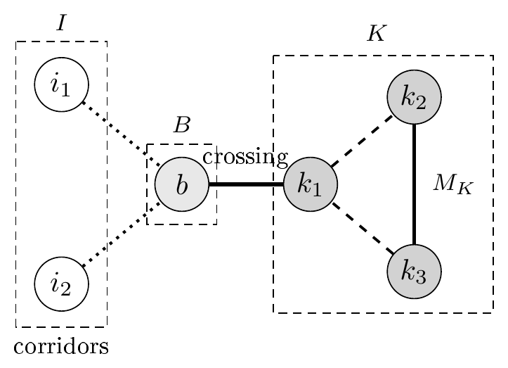
The main point of the paper is that this phenomenon is completely controlled by the matching interface across the Larson cut. We prove a normal form for maximum matchings: every maximum matching of \(G\) consists of a maximum matching on \(G[K]\) , a matching from a subset \(X\subseteq B\) into vertices exposed by that matching on \(K\) , and a maximum matching of the residual graph \(G[L-X]\) . The sets \(X\) that can occur in this way are called crossing profiles.
Once a crossing profile \(X\) is fixed, every maximum matching \(P\) of \(G[L-X]\) can be viewed as a matching of \(G[L]\) . The vertices exposed by \(P\) in \(G[L]\) are precisely the crossed boundary vertices \(X\) together with the vertices exposed in \(G[L-X]\) . The vertices of \(L\) that can be reached by \(P\) -augmenting paths in \(G[L]\) , over all crossing profiles and all residual maximum matchings, form a set \(\Lambda_I(G)\) . Our main theorem states that \[\operatorname{SD}(G)=K\cup\Lambda_I(G),\qquad \operatorname{KE}(G)=L\setminus\Lambda_I(G).\]
Thus the SD vertices on the Larson König–Egerváry side are not defined by searching again for flowers or posies; they are exactly the vertices reached by augmenting corridors created by admissible crossings of maximum matchings.
The paper is organized as follows. Section 2 contains the terminology and the standard tools used throughout the paper. Section 3 proves the normal form for maximum matchings with respect to the Larson decomposition. Section 4 proves that the Larson complement is contained in \(\operatorname{SD}(G)\) , using explicit alternating trees and only the classical notions of flower and posy. Section 5 records that any maximum-matching edge crossing the Larson boundary lies in a flower. Section 6 proves the matching-interface characterization of \(\operatorname{SD}(G)\) and \(\operatorname{KE}(G)\) . Finally, Section 7 rederives, as an application of our approach, the known forbidden SD–KE cut: no maximum matching of \(G\) contains an edge between \(\operatorname{SD}(G)\) and \(\operatorname{KE}(G)\) .
All graphs considered in this paper are finite, undirected, and simple. For any undefined terminology or notation, we refer the reader to Lovász and Plummer [ 20 ] or Diestel [ 5 ] .
For a graph \(G\) we write \(V(G)\) and \(E(G)\) for its vertex and edge sets. If \(X\subseteq V(G)\) , then \(G[X]\) denotes the subgraph induced by \(X\) , and \(N_G(X)\) denotes the open neighborhood of \(X\) in \(G\) . When \(X=\{x\}\) , we write \(N_G(x)\) for \(N_G(\{x\})\) . If \(X,Y\subseteq V(G)\) are disjoint, then \[E_G(X,Y)=\{xy\in E(G):x\in X,\ y\in Y\}.\]
A set \(S\subseteq V(G)\) is independent if no two vertices of \(S\) are adjacent, and \(\alpha(G)\) is the maximum cardinality of an independent set. A graph \(G\) is König–Egerváry if \[\alpha(G)+\mu(G)=|V(G)|.\]
A graph \(H\) will be called strict Hall , or \(2\) -bicritical , if \[|N_H(S)|>|S|,\] for every non-empty independent set \(S\subseteq V(H)\) . This is the form of \(2\) -bicriticality used throughout the paper.
A matching \(M\) in \(G\) is a set of pairwise disjoint edges. A vertex is \(M\) -saturated if it is incident with an edge of \(M\) , and \(M\) -exposed otherwise. The set of \(M\) -exposed vertices of a graph \(H\) is sometimes denoted by \[U_H(M)=\{v\in V(H): v\text{ is }M\text{-exposed}\}.\]
The size of a maximum matching of \(G\) is denoted by \(\mu(G)\) , and \(\mathcal M(G)\) is the set of maximum matchings of \(G\) . If \(v\) is \(M\) -saturated, its unique \(M\) -mate is denoted by \(M(v)\) . An edge is allowed if it belongs to at least one maximum matching of \(G\) . If \(M\) and \(N\) are matchings, then \(M\triangle N\) denotes their symmetric difference; every component of \(M\triangle N\) is an alternating path or an alternating cycle whose edges alternate between \(M\) and \(N\) .
A path \(P=p_0p_1\ldots p_t\) is always assumed to be simple. Its endpoints are \(p_0\) and \(p_t\) , its internal vertices are \(p_1,\ldots,p_{t-1}\) , and the reverse path is denoted by \(P^{-1}\) . A walk may repeat vertices and edges. Let \(M\) be a matching. An \(M\) -alternating path is a path whose consecutive edges alternate between edges of \(M\) and edges outside \(M\) . An \(M\) -alternating walk is defined similarly, allowing repetitions. For a non-trivial alternating path or walk we use the terminal types \[nm, \qquad nn, \qquad mm,\] according to whether the first and last edges are respectively outside/inside, outside/outside, or inside/inside \(M\) . Thus a path has type \(nm\) if its first edge is not in \(M\) and its last edge is in \(M\) , and similarly for the other two types.
The terminal type is always read in the displayed orientation of the path or walk and always with respect to the fixed matching under discussion. Thus an \(nm\) path from \(a\) to \(b\) need not be an \(nm\) path from \(b\) to \(a\) ; after reversal its first and last edge memberships are reversed. Whenever a later proof uses a terminal type, the path is first oriented in the direction in which the type is being asserted. The types \(nn\) and \(mm\) are invariant under reversal, but the orientation still specifies which endpoint is being treated as the initial endpoint in the argument.
An \(M\) -augmenting path is an \(M\) -alternating path whose two endpoints are \(M\) -exposed. Berge’s lemma will be used in the standard form: a matching is maximum if and only if it has no augmenting path [ 1 , 20 ] .
We shall also use the standard switching operation. If \(Q\) is an \(M\) -alternating even cycle, then \[M\triangle E(Q),\] is again a matching of the same cardinality as \(M\) . If \(Q\) is an \(M\) -augmenting path, then \(M\triangle E(Q)\) is a matching of size \(|M|+1\) . More generally, switching along an alternating path exchanges the matching and non-matching edges on that path whenever the result is a matching; the particular instances used below are the even-cycle and augmenting-path cases.
Let \(M\) be a maximum matching of \(G\) . An odd cycle \(C\) of length \(2k+1\) is an \(M\) -blossom if it contains exactly \(k\) edges of \(M\) . The unique vertex of \(C\) not saturated by \(M\cap E(C)\) is the base of the blossom. The base may still be saturated by \(M\) through an edge outside the cycle.
An \(M\) -flower is the union of an \(M\) -blossom \(C\) , with base \(b\) , and an \(M\) -alternating path \(P\) from an \(M\) -exposed vertex \(r\) to \(b\) , internally disjoint from \(C\) , such that \(P\) is trivial or has type \(nm\) when oriented from \(r\) to \(b\) . The path \(P\) is the stem of the flower. Equivalently, if the stem is non-trivial and is oriented from the base toward the exposed vertex, then it starts with an edge of \(M\) and ends with an edge outside \(M\) . The trivial stem can occur only when the base itself is \(M\) -exposed.
An \(M\) -posy is the union of two \(M\) -blossoms \(C_1,C_2\) , with bases \(b_1,b_2\) , and a non-trivial \(M\) -alternating path \(P\) from \(b_1\) to \(b_2\) , internally disjoint from \(C_1\cup C_2\) , such that \(P\) has type \(mm\) . The path \(P\) is the connector of the posy. The two blossoms need not be disjoint from each other; the connector is required to be a simple alternating path whose first and last edges belong to \(M\) .
Define \[\begin{aligned} \operatorname{SD}(G)=\{v\in V(G):&\ \text{there are }M\in\mathcal M(G)\text{ and an }M\text{-flower}\text{ or}\\ &\ \text{an }M\text{-posy }\mathcal Q\text{ with }v\in V(\mathcal Q)\}, \end{aligned}\] and \[\operatorname{KE}(G)=V(G)\setminus \operatorname{SD}(G).\]
This is the precise version of the informal description in the introduction: “lying in a flower or posy” means existence of at least one maximum matching and at least one corresponding classical witness. The base of a blossom is always the unique vertex not saturated by the matching edges on the blossom cycle itself; it may nevertheless be saturated in the ambient graph by the stem, by a posy connector, or by another matching edge outside the cycle. When a base is later called exposed, that statement refers to the ambient matching in the ambient graph, not merely to the cycle.
We shall use Theorem 1.1 as the classical Sterboul–Deming criterion throughout the paper.
For an independent set \(S\) of \(G\) , define its difference by \[d_G(S)=|S|-|N_G(S)|.\]
An independent set \(I\) is critical if it maximizes \(d_G(S)\) among all independent sets \(S\) of \(G\) . It is maximum critical if it has maximum cardinality among the critical independent sets. We allow the empty independent set; this is convenient when the maximum value of the difference is \(0\) . We write \(I\in\operatorname{MaxCrit}(G)\) when \(I\) is maximum critical.
The Larson decomposition is the following independence decomposition [ 17 , 27 ] .
Theorem 2.1 (Larson decomposition). Let \(I\in\operatorname{MaxCrit}(G)\) and put \[L(G)=I\cup N_G(I),\qquad L^c(G)=V(G)\setminus L(G).\]
Then \(L(G)\) is independent of the choice of \(I\) . Moreover, if \(K=L^c(G)\) , then:
(i) \(G[L(G)]\) is König–Egerváry;
(ii) \(I\) is a maximum independent set of \(G[L(G)]\) ;
(iii) \(G[K]\) is strict Hall, that is, \[|N_{G[K]}(S)|>|S|,\] for every non-empty independent set \(S\subseteq K\) .
The assertions imported from Larson and Pulleyblank are exactly the independence of \(L(G)\) from the chosen maximum critical independent set, the König–Egerváry structure of \(G[L(G)]\) with \(I\) maximum independent there, and the strict-Hall condition on \(G[L^c(G)]\) . The normal form for maximum matchings, the crossing profiles, the active set \(\Lambda_I(G)\) , and the identification with the SD–KE decomposition are consequences proved in the present paper. Although \(L(G)\) is independent of \(I\) at this point, the notation \(\Lambda_I(G)\) is allowed to depend on the chosen \(I\) until Theorem 6.7 , where its independence is obtained as a consequence of the main equality.
We shall use the induced-graph notation \[L_G=G[L(G)],\qquad L^c_G=G[L^c(G)].\]
Once a maximum critical independent set \(I\) has been fixed, we also use the abbreviations \[B=N_G(I),\qquad L=I\cup B, \qquad K=V(G)\setminus L.\]
There are no edges between \(I\) and \(K\) : by definition, every neighbor of a vertex of \(I\) belongs to \(B=N_G(I)\) . Consequently, every edge of \(G\) which is not contained in \(G[K]\) is incident with at least one vertex of \(B\) . This elementary observation is used repeatedly in the normal form for maximum matchings.
Throughout this section, fix \(I\in\operatorname{MaxCrit}(G)\) and write \[B=N_G(I),\qquad L=I\cup B, \qquad K=V(G)\setminus L.\]
There are no edges between \(I\) and \(K\) , by the definition of \(B\) , and \(I\) is independent. Consequently, every edge of \(G\) not contained in \(G[K]\) is incident with at least one vertex of \(B\) .
Lemma 3.1 (Deleting boundary vertices). For every \(X\subseteq B\) , the graph \(G[L-X]\) is König–Egerváry and \[\mu(G[L-X])=|B|-|X|.\]
In particular, every maximum matching of \(G[L-X]\) saturates all vertices of \(B\setminus X\) and uses no edge inside \(B\setminus X\) ; equivalently, every edge of such a matching joins \(B\setminus X\) to \(I\) .
Proof. By Theorem 2.1 , \(G[L]\) is König–Egerváry and \(I\) is a maximum independent set in \(G[L]\) . Hence \[\mu(G[L])=|L|-|I|=|B|.\]
Choose a maximum matching \(M_0\) of \(G[L]\) . Every edge of \(G[L]\) touches \(B\) , because \(I\) is independent and \(L=I\cup B\) . Since \(M_0\) has \(|B|\) disjoint edges, and each of these edges touches at least one vertex of \(B\) , the \(|B|\) edges of \(M_0\) must touch exactly the \(|B|\) vertices of \(B\) , one vertex of \(B\) per edge. In particular, no edge of \(M_0\) has both endpoints in \(B\) , and every edge of \(M_0\) joins a vertex of \(B\) to a vertex of \(I\) .
Now restrict \(M_0\) to the unique matching edges incident with the vertices of \(B\setminus X\) . None of these edges meets \(X\) , because the edges just described join \(B\) to \(I\) . They are still pairwise disjoint, and therefore form a matching of \(G[L-X]\) of size \(|B|-|X|\) . This proves \[\mu(G[L-X])\ge |B|-|X|.\]
The reverse inequality is immediate: every edge of \(G[L-X]\) touches \(B\setminus X\) , so a matching in \(G[L-X]\) has at most one edge for each vertex of \(B\setminus X\) . Thus \(\mu(G[L-X])=|B|-|X|\) .
If \(P\) is any maximum matching of \(G[L-X]\) , then \(|P|=|B|-|X|\) , and every edge of \(P\) touches \(B\setminus X\) . The same counting argument forces each edge of \(P\) to touch exactly one vertex of \(B\setminus X\) and forces all vertices of \(B\setminus X\) to be saturated by \(P\) . Hence \(P\) has no edge inside \(B\setminus X\) , and, because \(I\) is independent, every edge of \(P\) joins \(B\setminus X\) to \(I\) .
Moreover, \(I\) remains independent in \(G[L-X]\) , and no independent set of \(G[L-X]\) is larger than \(I\) , since \(I\) is maximum in \(G[L]\) . Therefore \(\alpha(G[L-X])=|I|\) , and \[\alpha(G[L-X])+\mu(G[L-X]) =|I|+|B|-|X| =|V(G[L-X])|.\]
Thus \(G[L-X]\) is König–Egerváry. \(\square\)
Lemma 3.2 (Larson count). One has \[\mu(G)=|B|+\mu(G[K]).\]
Proof. Every edge of \(G\) not contained in \(G[K]\) touches \(B\) . Hence any matching of \(G\) has at most \(|B|\) edges outside \(G[K]\) , and at most \(\mu(G[K])\) edges inside \(G[K]\) . Therefore \[\mu(G)\le |B|+\mu(G[K]).\]
By Lemma 3.1 , \(\mu(G[L])=|B|\) . The union of a maximum matching of \(G[L]\) and a maximum matching of \(G[K]\) has size \(|B|+\mu(G[K])\) , giving equality. \(\square\)
Proposition 3.3 (Normal form). Let \(M\in\mathcal M(G)\) . Then:
(a) \(M_K=M\cap E(G[K])\) is a maximum matching of \(G[K]\) ;
(b) \(M\) has exactly \(|B|\) edges outside \(E(G[K])\) ;
(c) each of those \(|B|\) edges contains exactly one vertex of \(B\) ; in particular, \(M\) saturates all vertices of \(B\) and uses no edge inside \(B\) ;
(d) if \[X_M=\{b\in B: M(b)\in K\},\] then the vertices \(M(X_M)\subseteq K\) are \(M_K\) -exposed;
(e) if \[H_M=G[L-X_M],\qquad M_L=M\cap E(H_M),\] then \(M_L\) is a maximum matching of \(H_M\) , and \(H_M\) is König–Egerváry.
Conversely, let \(M_K\) be a maximum matching of \(G[K]\) . Let \(X\subseteq B\) and let \(F\subseteq E_G(B,K)\) be a matching which saturates \(X\) and whose \(K\) -endpoints are \(M_K\) -exposed; in particular, the crossing edges are pairwise disjoint and use only vertices exposed by the selected matching \(M_K\) on \(G[K]\) . If \(P\) is a maximum matching of \(G[L-X]\) , then \(M_K\cup F\cup P\) is a maximum matching of \(G\) .
Proof. By Lemma 3.2 , a maximum matching must attain both bounds used in that lemma: it has \(\mu(G[K])\) edges inside \(K\) and \(|B|\) edges outside \(K\) . This gives (a) and (b).
Every edge outside \(K\) touches at least one vertex of \(B\) . Since the \(|B|\) such edges are disjoint, they touch at least \(|B|\) distinct vertices of \(B\) . As \(B\) has exactly \(|B|\) vertices, they touch all vertices of \(B\) , and each such edge touches exactly one of them. In particular, no edge of \(M\) lies inside \(B\) . This proves (c).
If \(b\in X_M\) and \(M(b)=z\in K\) , then \(z\) is not saturated by any edge of \(M_K\) ; otherwise \(z\) would be saturated twice by \(M\) . This proves (d).
The matching \(M_L\) has exactly \(|B|-|X_M|\) edges, because the vertices of \(B\setminus X_M\) are saturated inside \(L\) . By Lemma 3.1 , \[\mu(H_M)=\mu(G[L-X_M])=|B|-|X_M|,\] and \(H_M\) is König–Egerváry. Thus \(M_L\) is maximum in \(H_M\) , proving (e).
For the converse, take \(M_K\) , \(X\) , \(F\) , and \(P\) as in the statement. The hypotheses on \(F\) ensure that no vertex is used twice: the \(K\) -endpoints of \(F\) are exposed by \(M_K\) , the \(B\) -endpoints of \(F\) are exactly \(X\) , and \(P\) is contained in \(G[L-X]\) . Hence \(M_K\cup F\cup P\) is a matching. By Lemma 3.1 , \(|P|=|B|-|X|\) , so \[|M_K\cup F\cup P| =\mu(G[K])+|X|+|B|-|X| =\mu(G[K])+|B| =\mu(G),\] by Lemma 3.2 . Thus the union is a maximum matching of \(G\) . \(\square\)
The complement \(K=L^c(G)\) of Larson is \(2\) -bicritical. We now record the alternating facts that turn this strict Hall property into membership in \(\operatorname{SD}\) . All configurations produced in this section are classical flowers and posies in the sense of Theorem 1.1 ; no auxiliary variants are used.
Proposition 4.1 (Exposed vertices). Let \(H\) be \(2\) -bicritical. Let \(M\) be a maximum matching of \(H\) , and let \(r\) be an \(M\) -exposed vertex. Then there is an \(M\) -flower containing \(r\) . More precisely, there is a simple alternating path from \(r\) to the base of an \(M\) -blossom; if the path is non-trivial, its last edge belongs to \(M\) .
Proof. We give the construction of the Edmonds alternating tree rooted at \(r\) . Start with the trivial tree \(T_0\) whose only vertex is \(r\) . At every stage we have a rooted tree \(T\) such that, for each \(x\in V(T)\) , the unique path \(T[r,x]\) is simple and \(M\) -alternating. Since \(r\) is \(M\) -exposed, each non-trivial path \(T[r,x]\) starts with an edge outside \(M\) . A vertex of \(T\) is called outer if its distance from \(r\) in \(T\) is even, and inner if that distance is odd; in particular, \(r\) is outer.
The growth rule is the following. Suppose \(x\) is outer and there is an edge \(xy\in E(H)\) with \(y\notin V(T)\) . Then \(xy\notin M\) : if \(x\ne r\) , the vertex \(x\) is already matched in \(T\) to its inner parent, and if \(x=r\) , then \(r\) is \(M\) -exposed. If \(y\) were also \(M\) -exposed, the path \(T[r,x]\) followed by \(xy\) would be an augmenting path, contradicting the maximality of \(M\) . Hence \(y\) is \(M\) -saturated; write \(z=M(y)\) . The vertex \(z\) is not in \(T\) , because otherwise \(z\) would already be matched inside the tree or would be the exposed root. We therefore add the two edges \(xy\) and \(yz\) to \(T\) . The vertex \(y\) becomes inner and \(z\) becomes outer. This preserves the tree invariant: the new path to \(y\) is obtained from an alternating path ending at the outer vertex \(x\) by appending a non-matching edge, and the new path to \(z\) is obtained by appending the matching edge \(yz\) . Thus paths from \(r\) to outer vertices start outside \(M\) and, unless they are trivial, end in \(M\) , while paths from \(r\) to inner vertices start outside \(M\) and end outside \(M\) . We repeat this step until no extension is possible or an edge with both endpoints outer appears. Figure 2 illustrates the construction.
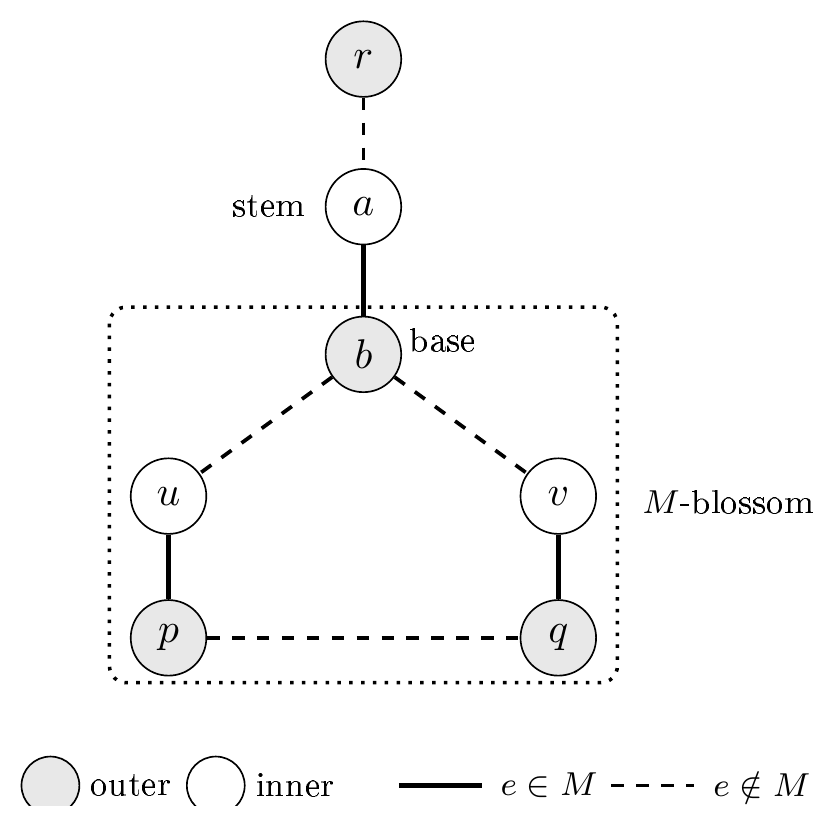
Assume, for a contradiction, that the search never finds an edge with both endpoints outer. Let \(T\) be a maximal alternating tree obtained in this way. Let \(X\) be the set of outer vertices of \(T\) , and let \(Y\) be the set of inner vertices.
First, \(X\) is independent. Indeed, if \(xy\) were an edge with \(x,y\in X\) , then letting \(b\) be the least common ancestor of \(x\) and \(y\) in \(T\) , the two branches \(T[b,x]\) and \(T[b,y]\) together with \(xy\) would form an odd alternating cycle with base \(b\) , namely an \(M\) -blossom. This contradicts our assumption.
Second, \[N_H(X)\subseteq Y.\]
For if \(w\in N_H(X)\) and \(xw\in E(H)\) with \(x\in X\) , then \(w\notin X\) by the previous paragraph. If \(w\notin V(T)\) , the growth rule would extend the tree from the outer vertex \(x\) , contradicting maximality. Thus \(w\in V(T)\setminus X\) , and by parity \(w\in Y\) .
Each vertex of \(Y\) is matched by \(M\) to a distinct vertex of \(X\setminus\{r\}\) : when an inner vertex enters the tree, its matching mate enters as an outer vertex. Conversely, every outer vertex except the root was introduced as the matching mate of an inner vertex. Hence \(|Y|=|X|-1\) for this tree; the weaker inequality \(|Y|\le |X|-1\) would also suffice. Since \(X\) is a non-empty independent set, strict Hall gives \(|N_H(X)|>|X|\) . The maximality of the search and the absence of outer–outer edges have just shown that every neighbor of \(X\) lies in \(Y\) , so \[|N_H(X)|\le |Y|=|X|-1,\] which is exactly the Hall contradiction.
Therefore the construction must find an outer–outer edge. If \(p\) and \(q\) are its endpoints and \(b\) is their least common ancestor in \(T\) , then \(T[b,p]\cup T[b,q]\cup\{pq\}\) is an \(M\) -blossom with base \(b\) . The path \(T[r,b]\) is simple and alternating; if non-trivial, it ends with an edge of \(M\) because \(b\) is outer. Together with the blossom, it is an \(M\) -flower containing \(r\) . \(\square\)
Lemma 4.2 (Forced-root alternating tree). Let \(H\) be \(2\) -bicritical. Let \(M\) be a maximum matching of \(H\) , and let \(x\) be a vertex saturated by every maximum matching of \(H\) . Then there are an \(M\) -blossom \(C\) , with base \(b\) , and a simple \(M\) -alternating path \(P\) from \(x\) to \(b\) , internally disjoint from \(C\) , such that \(P\) is trivial or has type \(mm\) .
Proof. Write \(u=M(x)\) . We run the same alternating-tree search as in Proposition 4.1 , except that the first edge is forced to be the matching edge \(xu\) . Start with the tree consisting of the edge \(xu\) . The vertex \(x\) is the root but is kept outside the parity classes; the vertex \(u\) is declared outer. In general, a vertex is outer if the tree path from \(x\) to it starts with \(xu\) and ends with an edge of \(M\) , and it is inner if that path starts with \(xu\) and ends with an edge outside \(M\) .
The growth rule is the usual one. If \(p\) is outer and \(pq\) is an edge with \(q\notin V(T)\) , then \(pq\notin M\) , because the matching mate of \(p\) is already its predecessor in the tree. If \(q\) were \(M\) -exposed, then the path from \(x\) to \(p\) followed by \(pq\) would be an alternating path starting with an edge of \(M\) and ending with an edge outside \(M\) . Such a path contains the same number of matching and non-matching edges. Switching \(M\) on it therefore gives another matching of the same cardinality: the initial matching edge \(xu\) is removed and no new edge is incident with \(x\) , while the final non-matching edge \(pq\) is added at the exposed endpoint \(q\) . The switched matching is maximum and leaves \(x\) exposed, contrary to the hypothesis. Thus \(q\) is \(M\) -saturated. We add \(pq\) and the matching edge \(qM(q)\) to the tree, putting \(q\) inner and \(M(q)\) outer. The invariant is the forced analogue of the invariant in Proposition 4.1 : paths from \(x\) to outer vertices start with \(xu\) and end in \(M\) , while paths from \(x\) to inner vertices start with \(xu\) and end outside \(M\) . We stop if an edge with both endpoints outer appears.
Assume, for a contradiction, that no outer–outer edge appears, and let \(T\) be a maximal tree obtained by the above procedure. Let \(X\) be the set of outer vertices and \(Y\) the set of inner vertices. The set \(X\) is non-empty, since \(u\in X\) , and \(X\) is independent; otherwise an edge between two outer vertices would have stopped the search and produced a blossom. Moreover, \[N_H(X)\subseteq Y\cup\{x\}.\]
Indeed, if a neighbor of an outer vertex were outside \(T\) , the growth rule would extend the tree; if it were another outer vertex, we would have an outer–outer edge. The only vertex of \(T\) which is neither outer nor inner is the root \(x\) .
Every inner vertex is matched by \(M\) to a distinct outer vertex different from \(u\) , and every outer vertex different from \(u\) arises in this way. Hence \(|Y|=|X|-1\) . Therefore \[|N_H(X)|\le |Y|+1=|X|,\] contradicting the \(2\) -bicritical inequality \(|N_H(X)|>|X|\) for the non-empty independent set \(X\) .
Thus the search finds an edge \(pq\) with both endpoints outer. Let \(b\) be the least common ancestor of \(p\) and \(q\) in the rooted tree. The root \(x\) has only the child \(u\) . Moreover, an inner vertex has only the one child added with it, namely its matching mate; branching can occur only at outer vertices, where non-matching edges are explored. Therefore the least common ancestor of two distinct outer vertices cannot be \(x\) and cannot be inner: if it were inner, both \(p\) and \(q\) would lie below the unique child of that inner vertex, contradicting the choice of the least common ancestor. Hence \(b\) is outer.
The two tree branches from \(b\) to \(p\) and \(q\) both have even length from \(b\) and start, when non-trivial, with non-matching edges. Adding the non-matching edge \(pq\) gives an odd alternating cycle with exactly one vertex not saturated by the matching edges on the cycle, namely \(b\) . Thus it is an \(M\) -blossom with base \(b\) . The tree path from \(x\) to \(b\) is simple, \(M\) -alternating, starts with the matching edge \(xu\) , and, if non-trivial, ends with an edge of \(M\) because \(b\) is outer. It is internally disjoint from the blossom by construction. \(\square\)
The next lemma is only a cleaning tool. It allows us to replace alternating walks that repeat vertices by classical flowers or posies with simple stems and connectors.
Lemma 4.3 (Cleaning alternating walks). Let \(G\) be a graph. In each of the following two situations the conclusion is only membership in \(\operatorname{SD}(G)\) : the final flower or posy may be taken with respect to a maximum matching obtained from the displayed matching by switching along even alternating cycles, and no assertion is made that the original matching or all vertices of the original walk are preserved.
(a) Let \(M\) be a maximum matching, let \(C\) be an \(M\) -blossom with base \(b\) , and let \(W\) be an \(M\) -alternating walk from an \(M\) -exposed vertex \(r\) to \(b\) . Suppose that \(W\) starts outside \(M\) , ends with an edge of \(M\) , and contains a vertex \(z\) . Then \(z\in \operatorname{SD}(G)\) .
(b) Let \(M\) be a maximum matching, let \(C_1,C_2\) be \(M\) -blossoms with bases \(b_1,b_2\) , and let \(W\) be an \(M\) -alternating walk from \(b_1\) to \(b_2\) . Suppose that \(W\) starts and ends with edges of \(M\) and contains a vertex \(z\) . Then \(z\in \operatorname{SD}(G)\) .
Proof. We argue simultaneously for (a) and (b). A witness means data of one of these two forms, with respect to some maximum matching \(N\) , whose alternating walk contains the fixed vertex \(z\) and has the prescribed terminal type. The initial hypotheses give at least one witness. Choose a witness for which the walk \(W\) has minimum length. The terminal blossoms and, in case (a), the exposed root are part of the witness, but the matching \(N\) is allowed to vary among maximum matchings during this minimization.
If \(W\) is a simple path, then the conclusion is immediate. In case (a), the path is a valid stem from an \(N\) -exposed root to the base of an \(N\) -blossom; in case (b), the path is a valid connector between the two blossom bases. Hence \(z\) lies in a classical flower or posy.
Assume now that \(W\) repeats a vertex. Choose two consecutive occurrences of a repeated vertex \(y\) and let \(D\) be the closed subwalk between them. By consecutiveness, \(D\) has no repeated internal vertex; hence \(D\) is a simple cycle. The alternating property implies the following dichotomy. If \(D\) has even length, then the two edges of \(D\) incident with \(y\) have opposite membership in \(N\) , so \(D\) is an even \(N\) -alternating cycle. If \(D\) has odd length, those two edges have the same membership. They cannot both lie in \(N\) , because \(N\) is a matching, so they both lie outside \(N\) ; in this case \(D\) is an \(N\) -blossom with base \(y\) .
First suppose that \(D\) is even. If \(z\notin V(D)\) , deleting the entire closed subwalk \(D\) gives a shorter alternating walk with the same endpoints and the same first and last edge memberships, contradicting minimality. Thus \(z\in V(D)\) . Switch \(N\) on the even alternating cycle \(D\) ; the result \(N’=N\triangle E(D)\) is a maximum matching. Let \(e^-\) and \(e^+\) be the edges of \(W\) immediately before the first occurrence of \(y\) and immediately after the second occurrence of \(y\) , omitting either one when \(y\) is an endpoint of \(W\) . Because the two \(D\) -edges incident with \(y\) have opposite \(N\) -membership, after the switch exactly one of the two \(y\) -arcs of \(D\) has the correct initial parity to follow \(e^-\) , and exactly one has the correct final parity to precede \(e^+\) . If these are different arcs, their union gives the original whole cycle; replacing one by the other removes at least one edge while keeping the part of \(D\) that contains \(z\) . If they are the same arc, that arc itself is a shorter \(N’\) -alternating replacement containing \(z\) . In all cases we obtain a witness, with respect to the maximum matching \(N’\) , whose walk still contains \(z\) and is strictly shorter than \(W\) . This contradicts the minimality of \(W\) . Hence an even repeated block cannot occur in a minimal witness.
Consequently \(D\) is odd, and \(D\) is an \(N\) -blossom with base \(y\) . There are two cases. If \(z\in V(D)\) , then the new blossom already contains \(z\) . In case (a), if the portion of \(W\) from the exposed root to \(y\) is used, it has the required stem parity after deleting any closed detours by the minimality argument above; if the other side is used, it connects \(y\) to the original terminal blossom. Thus \(D\) together with the appropriate exterior portion gives either a flower or a posy containing \(z\) . In case (b), the exterior portions from \(y\) to the two original blossom bases, when non-empty, start or end with matching edges in the required direction, so \(D\) and one of the original terminal blossoms form a posy, or \(D\) together with both exterior portions forms a posy. Hence \(z\in\operatorname{SD}(G)\) .
If \(z\notin V(D)\) , then \(z\) lies on exactly one exterior portion of \(W\) , say the portion between one terminal object and the occurrence of \(y\) . Replace the terminal object on the other side by the new blossom \(D\) and keep only the exterior portion containing \(z\) . The parity at \(y\) is correct because both cycle edges of \(D\) incident with the base \(y\) are outside \(N\) ; therefore the edge of the retained exterior portion incident with \(y\) , when present, has the matching membership required for a stem ending at a blossom base or for a connector ending at a blossom base. The resulting witness has the same type as one of (a) or (b), still contains \(z\) , and has a shorter walk than \(W\) , again contradicting minimality.
Thus the minimal witness is either already simple or immediately yields a classical flower or posy containing \(z\) . This proves \(z\in\operatorname{SD}(G)\) . \(\square\)
Proposition 4.4 (Vertices always saturated). Let \(H\) be \(2\) -bicritical. If \(x\) is saturated by every maximum matching of \(H\) , then \(x\) belongs to a flower or to a posy with respect to some maximum matching of \(H\) .
Proof. Fix a maximum matching \(M\) of \(H\) and write \(u=M(x)\) . By Lemma 4.2 applied to \(x\) , there are an \(M\) -blossom \(C_x\) , with base \(b_x\) , and a simple alternating path \[P_x:x,u,\ldots,b_x,\] of type \(mm\) , possibly ending already at \(u=b_x\) .
Suppose first that some maximum matching \(N\) exposes \(u\) . The component of \(M\triangle N\) containing \(u\) is an alternating path whose endpoint \(u\) is \(N\) -exposed and \(M\) -saturated. Since \(|M|=|N|\) , its other endpoint is an \(M\) -exposed vertex \(r\) . Oriented from \(r\) to \(u\) , this path starts outside \(M\) and ends with the edge \(xu\in M\) . Joining it with the subpath of \(P_x\) from \(u\) to \(b_x\) gives an alternating walk from the \(M\) -exposed vertex \(r\) to the base \(b_x\) which contains \(x\) . By Lemma 4.3 (a), \(x\) belongs to a flower or to a posy.
Suppose now that no maximum matching exposes \(u\) . Then \(u\) is also saturated by every maximum matching. Applying Lemma 4.2 to \(u\) , we obtain an \(M\) -blossom \(C_u\) , with base \(b_u\) , and a path \[P_u:u,x,\ldots,b_u,\] of type \(mm\) . Let \(R_x\) be the subpath of \(P_x\) from \(u\) to \(b_x\) . If \(R_x\) is non-trivial, then \(R_x^{-1}\) starts at \(b_x\) with an edge of \(M\) and ends at \(u\) with an edge outside \(M\) ; following it by \(P_u\) , which starts at \(u\) with the edge \(ux\in M\) and ends at \(b_u\) with an edge of \(M\) , gives an alternating walk of type \(mm\) from \(b_x\) to \(b_u\) containing \(x\) . If \(R_x\) is trivial, then \(b_x=u\) , and \(P_u\) itself is such a walk from \(b_x\) to \(b_u\) . By Lemma 4.3 (b), \(x\) belongs to a flower or to a posy. \(\square\)
Theorem 4.5 (2-bicritical graphs are SD). If \(H\) is \(2\) -bicritical, then \[\operatorname{SD}(H)=V(H).\]
Proof. Let \(x\in V(H)\) . If some maximum matching exposes \(x\) , apply Proposition 4.1 . Otherwise \(x\) is saturated by every maximum matching and Proposition 4.4 applies. In both cases \(x\) belongs to a flower or a posy with respect to some maximum matching. \(\square\)
Corollary 4.6 (The Larson complement is SD). For every graph \(G\) and every \(I\in\operatorname{MaxCrit}(G)\) , \[L^c(G)\subseteq \operatorname{SD}(G).\]
Proof. Let \(K=L^c(G)\) . If \(K=\varnothing\) , there is nothing to prove. By Larson, \(G[K]\) is \(2\) -bicritical. Given \(x\in K\) , Theorem 4.5 gives a maximum matching \(M_K\) of \(G[K]\) and a flower or posy contained in \(G[K]\) that contains \(x\) . By Lemma 3.2 , the union of \(M_K\) with a maximum matching of \(G[L]\) is a maximum matching of \(G\) . The same configuration remains a flower or posy in \(G\) , since it is entirely contained in \(K\) . Hence \(x\in\operatorname{SD}(G)\) . \(\square\)
The Larson boundary is not necessarily invisible to maximum matchings. The correct statement is stronger and more useful: whenever a maximum matching uses a Larson boundary edge, that edge lies in a flower entering \(L(G)\) from \(L^c(G)\) .
Theorem 5.1 (Boundary flowers). Let \(M\in\mathcal M(G)\) and let \(uv\in M\) with \(u\in L(G)\) and \(v\in L^c(G)\) . Then \(u\) and \(v\) belong to the same \(M\) -flower. In particular, \[u,v\in\operatorname{SD}(G).\]
Proof. Write \(B=N_G(I)\) , \(L=I\cup B\) , and \(K=L^c(G)\) . Since there are no edges between \(I\) and \(K\) , the endpoint \(u\) belongs to \(B\) . Moreover \(u\in X_M\) , and \(v\) is exposed by the maximum matching \(M_K=M\cap E(G[K])\) of \(G[K]\) .
By Proposition 4.1 , applied to the \(2\) -bicritical graph \(G[K]\) , there are an \(M_K\) -blossom \(C\) , with base \(b\) , and a simple alternating path \(P_K\) from \(v\) to \(b\) , contained in \(K\) , which starts outside \(M\) and, if non-trivial, ends with an edge of \(M\) .
Now set \[H^+=G[L-(X_M\setminus\{u\})].\]
The matching \(M_L=M\cap E(G[L-X_M])\) leaves \(u\) exposed in \(H^+\) . By Lemma 3.1 applied to \(X_M\setminus\{u\}\) , \[\mu(H^+)=|B|-|X_M|+1,\] whereas \(|M_L|=|B|-|X_M|\) . Berge’s lemma gives an augmenting path for \(M_L\) in \(H^+\) . This augmenting path must involve the only restored vertex \(u\) . Indeed, if neither endpoint were \(u\) , then all its vertices would lie in \(G[L-X_M]\) , and it would augment the maximum matching \(M_L\) there. Since \(u\) is \(M_L\) -exposed in \(H^+\) , it is one endpoint of the augmenting path. The other endpoint cannot lie in \(B\setminus X_M\) , because all vertices of \(B\setminus X_M\) are saturated by \(M_L\) ; it also cannot lie in \(X_M\setminus\{u\}\) , because those vertices are not present in \(H^+\) . Hence the other endpoint is an exposed vertex \(r\in I\) .
The vertex \(r\) is also \(M\) -exposed in the full graph \(G\) . It is not incident with a crossing edge, since there are no edges between \(I\) and \(K\) , and it is not saturated by \(M_L\) by construction of the augmenting path. Let \(P_L\) be this augmenting path oriented from \(r\) to \(u\) . Its first and last edges are outside \(M_L\) and, because all its edges lie in \(L\) , outside \(M\) as well.
The alternating path \[P_L,\ uv,\ P_K,\] is a simple \(M\) -alternating path: \(P_L\) is contained in \(L\) , \(P_K\) is contained in \(K\) , and they meet only through the edge \(uv\) . It starts at the \(M\) -exposed vertex \(r\) outside \(M\) and ends at the base \(b\) with an edge of \(M\) , unless \(P_K\) is trivial, in which case the last edge is \(uv\in M\) . Together with the blossom \(C\) , it is an \(M\) -flower containing \(u\) and \(v\) . \(\square\)
Remark 5.2. The weaker conclusion \(u,v\in\operatorname{SD}(G)\) will also follow from the final forbidden cut in Section 7 . The direct proof above is kept because it gives more: the two endpoints lie in one and the same flower, and the endpoint in \(L(G)\) therefore lies in a Larson corridor.
We now give the promised non-tautological description of the vertices of the Larson side \(L(G)\) that belong to \(\operatorname{SD}(G)\) . The definition uses only the normal form of maximum matchings and alternating paths inside the residual Larson side.
Fix \(I\in\operatorname{MaxCrit}(G)\) and write \[B=N_G(I),\qquad L=I\cup B, \qquad K=V(G)\setminus L.\]
If \(M_K\) is a maximum matching of \(G[K]\) , let \[U_K(M_K)=\{z\in K: z\text{ is }M_K\text{-exposed}\}.\]
A set \(X\subseteq B\) is called a crossing profile if there are a maximum matching \(M_K\) of \(G[K]\) and a matching \[F\subseteq E_G(B,K),\] which saturates \(X\) and whose \(K\) -endpoints lie in \(U_K(M_K)\) . Equivalently, \(X\) is a set of boundary vertices that can be matched across the Larson cut by some maximum matching of \(G\) . Let \(\mathfrak X_I\) denote the family of all crossing profiles.
For \(X\in\mathfrak X_I\) put \[H_X=G[L-X].\]
By Lemma 3.1 , \(H_X\) is König–Egerváry and every maximum matching of \(H_X\) has size \(|B|-|X|\) . If \(P\) is a maximum matching of \(H_X\) , let \[U_L(X,P)=\{u\in V(H_X):u\text{ is }P\text{-exposed}\}.\]
Since \(P\) saturates every vertex of \(B\setminus X\) , we have \[U_L(X,P)\subseteq I.\]
Definition 6.1 (Larson augmenting corridor). Let \(X\in\mathfrak X_I\) and let \(P\) be a maximum matching of \(H_X=G[L-X]\) . We view \(P\) as a matching of the larger graph \(G[L]\) . An \((X,P)\) -corridor is simply a \(P\) -augmenting path in \(G[L]\) .
Equivalently, an \((X,P)\) -corridor is a non-trivial simple \(P\) -alternating path whose endpoints are \(P\) -exposed in \(G[L]\) . These exposed vertices are precisely \[X\cup U_L(X,P),\] and the terminal edges of the path are outside \(P\) . All internal vertices of an augmenting path are \(P\) -saturated, so they cannot lie in \(X\cup U_L(X,P)\) . Hence, because \(P\) is a maximum matching of \(H_X=G[L-X]\) , no \((X,P)\) -corridor can have both endpoints in \(U_L(X,P)\) ; otherwise the whole path would be contained in \(H_X\) and would augment \(P\) there. Thus every corridor automatically has at least one endpoint in the crossed boundary set \(X\) .
Define the Larson-active set \[\Lambda_I(G)= \bigcup_{X\in\mathfrak X_I} \bigcup_{P\in\mathcal M(H_X)} \bigcup_{Q} V(Q),\] where \(Q\) ranges over all \((X,P)\) -corridors, equivalently over all \(P\) -augmenting paths in \(G[L]\) . This definition refers only to the possible crossing profiles of maximum matchings and to the augmenting-path structure that appears when a maximum matching of the residual König–Egerváry graph \(G[L-X]\) is viewed in the larger Larson side \(G[L]\) .
The description is meant as a structural and certificate-based reading of the SD–KE decomposition from the Larson interface. For a fixed maximum matching \(M_K\) of \(G[K]\) , the admissible profiles are exactly those subsets of \(B\) that can be matched in the bipartite graph between \(B\) and the exposed set \(U_K(M_K)\) . Once such an \(X\) is fixed, membership in the corresponding part of \(\Lambda_I(G)\) is certified by a maximum matching \(P\) of \(G[L-X]\) and an ordinary \(P\) -augmenting path in \(G[L]\) . Thus each positive membership claim has a finite matching-and-path certificate. We do not claim here that this is the most efficient algorithmic procedure; the purpose of the definition is to give a structural interface description that can be checked by standard matching certificates.
Lemma 6.2 (Crossing profiles are exactly the possible crossing sets). A set \(X\subseteq B\) belongs to \(\mathfrak X_I\) if and only if there is a maximum matching \(M\) of \(G\) such that \[X=\{b\in B:M(b)\in K\}.\]
For such an \(M\) , the restriction \(M\cap E(G[L-X])\) is a maximum matching of \(H_X\) .
Proof. If \(M\) is a maximum matching of \(G\) , the assertion follows from the normal form, Proposition 3.3 : the \(K\) -endpoints of the crossing edges are exposed by \(M\cap E(G[K])\) , and the residual part on \(L-X\) is maximum.
Conversely, suppose \(X\in\mathfrak X_I\) . Choose \(M_K\in\mathcal M(G[K])\) and a matching \(F\) from \(X\) into \(U_K(M_K)\) witnessing that \(X\) is a crossing profile. Let \(P\) be any maximum matching of \(H_X=G[L-X]\) . By Lemma 3.1 , \(|P|=|B|-|X|\) . The matching \[M=M_K\cup F\cup P,\] has size \(\mu(G[K])+|X|+|B|-|X|=\mu(G[K])+|B|=\mu(G)\) by Lemma 3.2 . Thus \(M\) is maximum and its crossing set is exactly \(X\) . \(\square\)
Lemma 6.3 (Corridors produce classical SD configurations). Every vertex of \(\Lambda_I(G)\) belongs to \(\operatorname{SD}(G)\) .
Proof. Let \(Q=q_0\ldots q_t\) be an \((X,P)\) -corridor. Choose a maximum matching \(M_K\) of \(G[K]\) and a crossing matching \(F\) witnessing \(X\in\mathfrak X_I\) , and set \[M=M_K\cup F\cup P.\]
By Lemma 6.2 , \(M\) is a maximum matching of \(G\) .
First assume that one endpoint of \(Q\) , say \(q_0=b\) , lies in \(X\) and the other endpoint \(q_t=u\) lies in \(U_L(X,P)\) . Let \(r=M(b)\in K\) . Then \(r\) is \(M_K\) -exposed. By Proposition 4.1 applied inside \(G[K]\) , there is an \(M_K\) -flower with exposed root \(r\) , blossom \(C\) , and base \(c\) . Reading its stem from \(c\) to \(r\) , then using the matching edge \(rb\) , and finally following the corridor \(Q\) from \(b\) to \(u\) , gives an \(M\) -alternating walk from the base \(c\) to the \(M\) -exposed vertex \(u\) . The first edge at \(c\) is a matching edge unless the stem in \(K\) is trivial, in which case the first edge is \(rb\in M\) ; the last edge at \(u\) is outside \(M\) because \(Q\) is \(P\) -augmenting. For an arbitrary vertex \(z\in V(Q)\) , the same walk contains \(z\) , so Lemma 4.3 (a), applied to this particular \(z\) , gives \(z\in\operatorname{SD}(G)\) .
Now assume that both endpoints of \(Q\) lie in \(X\) , say \(q_0=b_1\) and \(q_t=b_2\) . Let \(r_i=M(b_i)\in K\) for \(i=1,2\) . The vertices \(r_1,r_2\) are exposed by \(M_K\) . Applying Proposition 4.1 in \(G[K]\) to \(r_1\) and to \(r_2\) , and then joining the two stems with the matching edges \(r_1b_1\) , \(b_2r_2\) and with the corridor \(Q\) , gives an alternating walk of type \(mm\) between two blossom bases. Again, for each fixed \(z\in V(Q)\) this walk contains \(z\) , and Lemma 4.3 (b) gives \(z\in\operatorname{SD}(G)\) . The cleaning lemma is used here only as a membership statement, one vertex at a time; it is not required to preserve a single witness containing the whole corridor. Hence \(V(Q)\subseteq\operatorname{SD}(G)\) in all cases. \(\square\)
The converse is the point at which the König–Egerváry structure of the Larson side enters. We record the elementary terminal-type fact that will be used to reduce arbitrary flowers and posies to corridors.
Lemma 6.4 (Terminal types on the residual Larson side). Let \(X\subseteq B\) , let \(P\) be a maximum matching of \(H_X=G[L-X]\) , and let \(R\) be a simple \(P\) -alternating path contained in \(H_X\) . Then no subpath of \(R\) can have both endpoints in \(B\setminus X\) and have type \(mm\) .
Moreover, let \(M\in\mathcal M(G)\) have crossing set \(X\) and residual matching \(P=M\cap E(G[L-X])\) , and let \(\mathcal Q\) be an \(M\) -flower or an \(M\) -posy. Every maximal alternating segment of \(\mathcal Q\) lying in \(L\) can be enlarged within the same stem, connector, or blossom cycle until either its endpoints are \(P\) -exposed in \(G[L]\) , or one obtains a forbidden \(mm\) subpath in \(H_X\) between two vertices of \(B\setminus X\) . Consequently the second alternative cannot occur, and the enlarged segment is a \(P\) -augmenting path in \(G[L]\) .
Proof. By Lemma 3.1 , the matching \(P\) saturates every vertex of \(B\setminus X\) and every edge of \(P\) joins a vertex of \(B\setminus X\) to a vertex of \(I\) . Start at a vertex of \(B\setminus X\) and traverse an alternating path whose first edge belongs to \(P\) . The first matching edge goes from \(B\setminus X\) to \(I\) ; the following non-matching edge, if present, must leave \(I\) and therefore goes to \(B\setminus X\) , since \(I\) is independent. Inductively, every matching edge is traversed from \(B\setminus X\) to \(I\) . Hence such a path cannot end at a vertex of \(B\setminus X\) through a matching edge. This proves the first assertion.
We now prove the enlargement statement. Delete the vertices of \(K\) from the flower or posy \(\mathcal Q\) . What remains inside \(L\) is a disjoint union of vertices and simple alternating path segments, each lying on one of the following pieces of the witness: a flower stem, a posy connector, or a blossom cycle. On \(L-X\) , the matching edges of \(M\) are exactly the edges of \(P\) ; a vertex of \(X\) is \(P\) -exposed in \(G[L]\) because its \(M\) -mate lies in \(K\) , and a vertex of \(U_L(X,P)\) is \(P\) -exposed by definition.
Consider one endpoint \(a\) of such a segment. If \(a\in X\cup U_L(X,P)\) , then \(a\) is already a valid endpoint for a corridor. Suppose that \(a\) is not \(P\) -exposed. Then \(a\notin X\) and \(a\notin U_L(X,P)\) , so \(a\) is \(P\) -saturated. If \(a\in I\) , its unique \(P\) -mate lies in \(B\setminus X\) ; the matching edge to that mate is present whenever the witness continues through \(a\) as an internal vertex, as the endpoint of a non-trivial stem, or as the endpoint of a connector. Thus the segment was not maximal unless that matching edge is already included. Accordingly, a non-closed endpoint of a maximal segment may be treated as a vertex of \(B\setminus X\) reached through its \(P\) -edge. The same conclusion holds directly when \(a\in B\setminus X\) : if the terminal edge at \(a\) were outside \(P\) , the \(P\) -mate of \(a\) would be the next edge of the alternating witness unless \(a\) were an exposed root or a trivial-stem base, both impossible for a \(P\) -saturated boundary vertex. Hence every non-closed endpoint is an ordinary boundary vertex of \(B\setminus X\) , and the segment enters it through a matching edge of \(P\) .
The roles that can occur at a blossom base require the same convention used in Section 2.1 . A blossom base is not saturated by matching edges on the cycle, but if it is used by a non-trivial flower stem or by a posy connector, the incident stem or connector edge is in the ambient matching. Therefore an ordinary boundary base cannot be a closed endpoint: its matching edge is part of the stem or connector and must be included in the enlargement. A trivial flower stem has an ambient exposed base, hence gives a vertex of \(U_L(X,P)\) , while a crossed base lies in \(X\) . Thus bases, trivial stems, connector endpoints, ordinary boundary vertices, crossed boundary vertices, and residual exposed vertices are all covered by the preceding endpoint classification.
Starting with the segment that contains the vertex under consideration, extend at any non-closed endpoint along the same stem, connector, or blossom cycle through the forced matching edge just identified. The process stops only when an endpoint lies in \(X\cup U_L(X,P)\) , or when both endpoints of the current segment are ordinary boundary vertices of \(B\setminus X\) reached through matching edges. In the latter case the current segment contains a subpath in \(H_X\) of type \(mm\) with both endpoints in \(B\setminus X\) , contradicting the first assertion. Hence the only possible terminal vertices after enlargement are \(P\) -exposed vertices of \(G[L]\) . The enlarged segment is a simple \(P\) -alternating path whose terminal edges are outside \(P\) , and is therefore a \(P\) -augmenting path in \(G[L]\) . \(\square\)
Lemma 6.5 (Interface reduction). Let \(M\in\mathcal M(G)\) , let \(X=\{b\in B:M(b)\in K\}\) , and let \(P=M\cap E(G[L-X])\) . If an \(M\) -flower or an \(M\) -posy touches \(K\) and contains a vertex \(x\in L\) , then \(x\) lies on an \((X,P)\) -corridor.
Proof. Let \(\mathcal Q\) be such a flower or posy. By Proposition 3.3 , \(P\) is a maximum matching of \(H_X=G[L-X]\) . Remove from \(\mathcal Q\) all vertices of \(K\) and all edges incident with them. The remaining pieces in \(L\) are vertices or simple \(P\) -alternating paths: inside \(L-X\) the matching edges of \(M\) are precisely the edges of \(P\) , while each vertex of \(X\) has its matching edge in \(K\) and is therefore \(P\) -exposed when \(P\) is viewed in \(G[L]\) .
Let \(R\) be the remaining piece containing \(x\) . First suppose that \(R\) is the single vertex \(x\) . Since the original configuration touches \(K\) , the vertex \(x\) is incident in \(\mathcal Q\) only with edges whose other endpoints lie in \(K\) , or else \(R\) would contain a non-trivial edge of \(L\) . There are no edges between \(I\) and \(K\) , so \(x\in B\) . If \(x\in B\setminus X\) , then its matching edge under \(M\) is the edge of \(P\) joining \(x\) to a vertex of \(I\) . Such an edge would have to appear in the witness whenever \(x\) is a non-base vertex of a blossom, an internal vertex of a stem or connector, or an ordinary boundary base attached to a non-trivial stem or to a connector. The remaining base cases are also impossible for \(x\in B\setminus X\) : a trivial flower base is \(M\) -exposed, whereas \(x\) is \(P\) -saturated, and a base whose incident stem or connector edge leaves \(L\) through a matching edge is crossed. Hence the isolated vertex cannot come from an ordinary boundary role; it must be a crossed boundary vertex, so \(x\in X\) .
Put \[H^+=G[L-(X\setminus\{x\})].\]
By Lemma 3.1 , \(\mu(H^+)=|B|-|X|+1\) , whereas \(|P|=|B|-|X|\) . Berge’s lemma gives a \(P\) -augmenting path in \(H^+\) . This path must have \(x\) as an endpoint, because otherwise it would be contained in \(H_X\) and would augment the maximum matching \(P\) there. Since the path lies in \(G[L]\) , it is an \((X,P)\) -corridor containing \(x\) .
Assume now that \(R\) is non-trivial. If both endpoints of \(R\) are \(P\) -exposed in \(G[L]\) , then \(R\) itself is a \(P\) -augmenting path, hence an \((X,P)\) -corridor. If not, apply the enlargement procedure of Lemma 6.4 to the segment of the flower stem, posy connector, or blossom cycle containing \(R\) . The endpoint analysis in that lemma separately covers residual exposed vertices, crossed boundary vertices, ordinary boundary vertices, blossom bases, trivial stems, and connector endpoints. The only possible obstruction to reaching exposed endpoints would be an \(mm\) subpath of \(H_X\) between two ordinary boundary vertices of \(B\setminus X\) , which is forbidden by Lemma 6.4 . Thus \(R\) is contained in a simple \(P\) -alternating path in \(G[L]\) whose endpoints are \(P\) -exposed. This path is an \((X,P)\) -corridor and contains \(x\) . \(\square\)
Lemma 6.6 (No SD configuration is internal to L). Let \(M\in\mathcal M(G)\) , and let \(\mathcal Q\) be an \(M\) -flower or an \(M\) -posy. Then \[V(\mathcal Q)\nsubseteq L(G).\]
Equivalently, no SD configuration of \(G\) can live completely inside the Larson part \(L(G)\) .
Proof. Let \(X_M=\{b\in B:M(b)\in K\}\) . Suppose, for a contradiction, that \(V(\mathcal Q)\subseteq L\) .
We first show that \(\mathcal Q\) contains no vertex of \(X_M\) . If \(x\in X_M\) , its unique matching edge leaves \(L\) and goes to \(K\) . Consider the possible roles of \(x\) in a classical witness contained in \(L\) . If \(x\) is a non-base vertex of a blossom cycle, then one of the two cycle edges incident with \(x\) is the matching edge of the blossom, and that edge would have to lie in \(L\) . If \(x\) is an internal vertex of a flower stem or of a posy connector, then exactly one of the two incident path edges is its matching edge, again lying in \(L\) . Both possibilities contradict \(x\in X_M\) .
It remains to consider bases and endpoints. A flower with a trivial stem has an ambient exposed base, but every vertex of \(X_M\) is \(M\) -saturated by its crossing edge. A flower with a non-trivial stem reaches the base through the last stem edge, and that edge belongs to \(M\) . In a posy, each connector endpoint is a blossom base and the first and last connector edges belong to \(M\) . Thus a base of a non-trivial flower or of a posy would again need its matching edge inside \(L\) . These cases exhaust the roles of a vertex in a flower or posy, so \[V(\mathcal Q)\cap X_M=\varnothing.\]
Therefore \(\mathcal Q\) is actually contained in \(H_M=G[L-X_M]\) . On this graph the matching induced by \(M\) is \[M_L=M\cap E(H_M),\] and Proposition 3.3 says that \(M_L\) is a maximum matching of \(H_M\) and that \(H_M\) is König–Egerváry. Since no vertex of \(\mathcal Q\) lies in \(X_M\) , every matching edge used by the witness is an edge of \(M_L\) , and every exposed root or trivial-stem base that is exposed in \(G\) remains exposed in \(H_M\) . The same blossom cycles, stems, and connectors therefore form an \(M_L\) -flower or an \(M_L\) -posy in \(H_M\) . This contradicts the Sterboul–Deming criterion Theorem 1.1 , because a König–Egerváry graph has no such witness with respect to a maximum matching. Hence \(\mathcal Q\) cannot be contained in \(L\) . \(\square\)
Theorem 6.7 (SD–KE from the Larson matching interface). Let \(G\) be a graph and let \(I\in\operatorname{MaxCrit}(G)\) . Write \[L=L(G)=I\cup N_G(I),\qquad K=L^c(G)=V(G)\setminus L.\]
Let \(\Lambda_I(G)\) be the Larson-active set defined by crossing profiles and augmenting corridors. Then \[{\operatorname{SD}(G)=K\cup\Lambda_I(G)}, \qquad {\operatorname{KE}(G)=L\setminus\Lambda_I(G)}.\]
Equivalently, a vertex \(x\in L(G)\) belongs to \(\operatorname{SD}(G)\) if and only if, for some crossing profile \(X\) , some maximum matching \(P\) of \(G[L-X]\) , and some \(P\) -augmenting path \(Q\) in \(G[L]\) , one has \(x\in V(Q)\) .
Proof. By Corollary 4.6 , \(K\subseteq\operatorname{SD}(G)\) . By Lemma 6.3 , \(\Lambda_I(G)\subseteq\operatorname{SD}(G)\) . Hence \[K\cup\Lambda_I(G)\subseteq\operatorname{SD}(G).\]
Conversely, let \(x\in\operatorname{SD}(G)\) . If \(x\in K\) , there is nothing to prove. Assume \(x\in L\) . Choose a maximum matching \(M\) and an \(M\) -flower or \(M\) -posy \(\mathcal Q\) containing \(x\) . By Lemma 6.6 , the configuration \(\mathcal Q\) touches \(K\) . Let \(X=\{b\in B:M(b)\in K\}\) and \(P=M\cap E(G[L-X])\) . By Lemma 6.2 , \(X\) is a crossing profile and \(P\) is a maximum matching of \(G[L-X]\) . By Lemma 6.5 , the vertex \(x\) lies on an \((X,P)\) -corridor. Thus \(x\in\Lambda_I(G)\) .
Therefore \(\operatorname{SD}(G)=K\cup\Lambda_I(G)\) . Taking complements in the disjoint union \(V(G)=L\mathbin{\overset{\cdot}{\cup}} K\) gives \(\operatorname{KE}(G)=L\setminus\Lambda_I(G)\) . Since \(K\) and \(L\) are disjoint, the equality also gives the useful identity \[\Lambda_I(G)=\operatorname{SD}(G)\cap L(G).\] \(\square\)
Remark 6.8. The definition of \(\Lambda_I(G)\) no longer refers to flowers or posies. It uses only the possible crossing sets of maximum matchings across the Larson cut and the ordinary augmenting paths that appear when a maximum matching of the residual König–Egerváry graph \(G[L-X]\) is viewed inside \(G[L]\) . This is the sense in which the theorem reads the SD–KE decomposition from Larson rather than simply restating the definition of \(\operatorname{SD}(G)\) . In addition, because Larson’s theorem makes \(L(G)\) independent of the chosen maximum critical independent set and because \(\operatorname{SD}(G)\) is intrinsic, the identity \(\Lambda_I(G)=\operatorname{SD}(G)\cap L(G)\) shows that the active set is independent of the chosen \(I\in\operatorname{MaxCrit}(G)\) , even though its definition was made through that choice.
The interface theorem has already put the SD–KE partition in Larson coordinates: \[\operatorname{SD}(G)=K\cup\Lambda_I(G),\qquad \operatorname{KE}(G)=L\setminus\Lambda_I(G).\]
Thus the forbidden cut is equivalent to saying that the Larson-active side \(K\cup\Lambda_I(G)\) is closed under allowed edges. The forbidden cut was stated in [ 14 ] ; here it is included not as a new statement, but as a self-contained derivation from the Larson matching interface. This application shows that the interface theorem is strong enough to recover the classical separation between the SD side and the KE side along maximum matchings. We prove this closure using only two short transport facts for classical flowers and posies, and then apply Theorem 6.7 .
Lemma 7.1 (Local absorption by a classical witness). Let \(M\) be a maximum matching and let \(\mathcal Q\) be an \(M\) -flower or an \(M\) -posy. Then the following hold.
(a) If \(x\in V(\mathcal Q)\) and \(x\) is \(M\) -saturated, then \(M(x)\in V(\mathcal Q)\) .
(b) Let \(P=p_0p_1\ldots p_t\) be a simple \(M\) -alternating path whose internal vertices do not belong to \(\mathcal Q\) . Suppose that the terminal edges of \(P\) are outside \(M\) . If either both endpoints of \(P\) lie in \(V(\mathcal Q)\) , or one endpoint is \(M\) -exposed and the other lies in \(V(\mathcal Q)\) , then every vertex of \(P\) belongs to \(\operatorname{SD}(G)\) .
Proof. For (a), consider the possible positions of \(x\) in the witness. On a blossom cycle, every non-base vertex is saturated by the unique matching edge of the cycle incident with it, so its mate is the adjacent vertex on the same blossom. On the interior of a stem or connector, the matching mate is the adjacent vertex on the same alternating path. At a blossom base the cycle itself does not saturate the base. If the base is the root of a trivial flower stem, it is not \(M\) -saturated, so it is irrelevant to (a). If the flower stem is non-trivial, the last stem edge incident with the base belongs to \(M\) , and the mate lies on the stem. In a posy, the first and last connector edges belong to \(M\) , so the mate of each base lies on the connector. These cases exhaust all vertices of a flower or posy, proving \(M(x)\in V(\mathcal Q)\) whenever \(x\in V(\mathcal Q)\) is \(M\) -saturated.
For (b), let an endpoint of \(P\) that lies in \(V(\mathcal Q)\) be called an entry point. The edge of \(P\) incident with an entry point is outside \(M\) by hypothesis. We describe the possible alternating continuations inside \(\mathcal Q\) after such an outside edge.
If the entry point lies on a blossom cycle and is not the base, then exactly one of the two directions around the odd cycle begins with the matching edge incident with the entry point. Following that direction gives a simple alternating path to the blossom base; the terminal edge at the base is outside \(M\) if the path uses the whole alternating side of the cycle, and otherwise the base is reached as the unsaturated vertex of the blossom. If the entry point is the base, the continuation may be taken to be trivial at the base. If the entry point lies on a flower stem, one follows the stem in the direction compatible with alternation: either toward the exposed root, where the final edge is outside \(M\) , or toward the blossom base, where the final edge is in \(M\) . If the entry point lies on a posy connector, one follows the connector in the compatible direction until one of its blossom bases is reached; because a connector has type \(mm\) , the endpoint edge at that base belongs to \(M\) . These alternatives give the required case distinctions for flowers and posies.
Concatenate \(P\) with the appropriate internal continuations from its entry point or entry points. If one end of the resulting alternating walk is an exposed root and the other is a blossom base, Lemma 4.3 (a) applies to every prescribed vertex of \(P\) . If the two distinguished ends are blossom bases, Lemma 4.3 (b) applies. If both distinguished ends are exposed roots, then the alternating walk starts and ends outside \(M\) ; a simple such walk would be an \(M\) -augmenting path, impossible because \(M\) is maximum. Hence a first repetition occurs, and the first odd repeated block yields an \(M\) -blossom whose base is connected to one of the exposed roots by an alternating stem; equivalently, this is the flower case covered by Lemma 4.3 (a). Applying the cleaning lemma separately to each fixed vertex of \(P\) gives that every vertex of \(P\) lies in \(\operatorname{SD}(G)\) . \(\square\)
Lemma 7.2 (Symmetric-difference transport). Let \(M,N\in\mathcal M(G)\) , let \(\mathcal Q\) be an \(N\) -flower or an \(N\) -posy, and let \(R\) be a component of \(M\triangle N\) . If \[V(R)\cap V(\mathcal Q)\ne\varnothing,\] then \(V(R)\subseteq\operatorname{SD}(G)\) .
Proof. The component \(R\) is an alternating cycle or an alternating path whose edges alternate between \(M\) and \(N\) . Since both matchings are maximum, \(R\) has the same number of \(M\) -edges and \(N\) -edges. Otherwise switching the larger side of \(R\) into the smaller one would increase the cardinality of one of the two maximum matchings. Therefore \[N_R=N\triangle E(R),\] is again a maximum matching.
Decompose \(R\) into maximal subpaths whose internal vertices lie outside \(\mathcal Q\) and whose endpoints, when they exist, are either vertices of \(\mathcal Q\) or endpoints of the path component \(R\) . Let \(S\) be such a subpath with an endpoint \(q\in V(\mathcal Q)\) . The edge of \(S\) incident with \(q\) cannot be an \(N\) -edge: if it were, then by Lemma 7.1 (a) its other endpoint, the \(N\) -mate of \(q\) , would also belong to \(V(\mathcal Q)\) , contradicting the maximality of \(S\) unless \(S\) had length zero. Hence every non-trivial subpath enters or leaves \(\mathcal Q\) through an edge outside \(N\) .
If a subpath \(S\) has two endpoints in \(V(\mathcal Q)\) , then both terminal edges of \(S\) are outside \(N\) , and Lemma 7.1 (b), applied with the matching \(N\) , gives \(V(S)\subseteq\operatorname{SD}(G)\) . If \(R\) is a path and a subpath \(S\) has one endpoint in \(V(\mathcal Q)\) and the other endpoint is \(N\) -exposed, then the same lemma applies, again with respect to \(N\) . These cases absorb all internal bridges through \(R\) and every tail that starts at an \(N\) -exposed endpoint of \(R\) .
It remains to treat the only tail not covered by the previous paragraph: a path subcomponent \(S\) that starts at a vertex \(q\in V(\mathcal Q)\) , leaves \(\mathcal Q\) through an edge outside \(N\) , and ends at the other endpoint of \(R\) , which is not \(N\) -exposed. Switch on the whole component \(R\) and use the maximum matching \(N_R\) . With respect to \(N_R\) , the first edge of this tail, read from \(q\) , is a matching edge, and the final endpoint of the tail is \(N_R\) -exposed. The portion of \(\mathcal Q\) that formerly supplied the alternating continuation from \(q\) can be replaced by this switched edge; if this creates repeated vertices, the cleaning lemma Lemma 4.3 removes the repetitions and yields an \(N_R\) -flower or an \(N_R\) -posy containing \(q\) . Now the same tail is an alternating path whose terminal edge at \(q\) is outside that cleaned witness and whose other endpoint is \(N_R\) -exposed, so Lemma 7.1 (b), applied with the matching \(N_R\) , gives that all vertices of the tail lie in \(\operatorname{SD}(G)\) .
Every vertex of \(R\) lies in one of the maximal subpaths just considered. Hence \(V(R)\subseteq\operatorname{SD}(G)\) . \(\square\)
Proposition 7.3 (Closure of the Larson-active side under maximum-matching edges). Fix \(I\in\operatorname{MaxCrit}(G)\) and use the notation of Theorem 6.7 . Let \(xy\in E(G)\) be an edge that belongs to at least one maximum matching of \(G\) . If \[x\in K\cup\Lambda_I(G),\] then \[y\in K\cup\Lambda_I(G).\]
Proof. Choose a maximum matching \(M\) of \(G\) such that \(xy\in M\) . If \(y\in K\) , there is nothing to prove; assume \(y\in L\) .
If \(x\in K\) , then \(xy\) is a Larson boundary edge used by a maximum matching. By Theorem 5.1 , the endpoint \(y\) lies in a classical flower, so \(y\in\operatorname{SD}(G)\) . Since \(y\in L\) , the interface theorem Theorem 6.7 gives \(y\in\Lambda_I(G)\) .
Now assume \(x\in\Lambda_I(G)\) . By Lemma 6.3 , \(x\in\operatorname{SD}(G)\) ; choose a maximum matching \(N\) and an \(N\) -flower or \(N\) -posy \(\mathcal Q\) containing \(x\) . If \(xy\in N\) , then Lemma 7.1 (a) gives \(y\in V(\mathcal Q)\subseteq\operatorname{SD}(G)\) . If \(xy\notin N\) , let \(R\) be the component of \(M\triangle N\) containing \(xy\) . Since \(xy\in M\setminus N\) and \(x\in V(\mathcal Q)\) , we have \(V(R)\cap V(\mathcal Q)\ne\varnothing\) . Hence Lemma 7.2 gives \(y\in\operatorname{SD}(G)\) . Again \(y\in L\) , so Theorem 6.7 implies \(y\in\Lambda_I(G)\) . \(\square\)
The next statement is the forbidden SD–KE cut. It was previously stated in [ 14 ] ; the contribution here is not the statement itself, but an independent derivation from the Larson matching interface. Thus the result functions as an application and consistency check of Theorem 6.7 , not as an additional external input to the proof of the main theorem.
Theorem 7.4 (Forbidden SD–KE cut; rederived from the Larson interface). Let \(G\) be a graph. No edge joining \(\operatorname{SD}(G)\) to \(\operatorname{KE}(G)\) belongs to a maximum matching of \(G\) . Equivalently, for every maximum matching \(M\) of \(G\) , \[M\cap E_G(\operatorname{SD}(G),\operatorname{KE}(G))=\varnothing.\]
In other words, if \(u\in\operatorname{SD}(G)\) , \(v\in\operatorname{KE}(G)\) , and \(uv\in E(G)\) , then \(uv\notin M\) for every maximum matching \(M\) of \(G\) .
Proof. Fix \(I\in\operatorname{MaxCrit}(G)\) and write \(L=L(G)\) , \(K=L^c(G)\) . By Theorem 6.7 , \[\operatorname{SD}(G)=K\cup\Lambda_I(G),\qquad \operatorname{KE}(G)=L\setminus\Lambda_I(G).\]
Suppose, to the contrary, that there exist \(u\in\operatorname{SD}(G)\) , \(v\in\operatorname{KE}(G)\) , and a maximum matching \(M\) of \(G\) such that \(uv\in M\) . Then \[u\in K\cup\Lambda_I(G),\qquad v\in L\setminus\Lambda_I(G).\]
Since the edge \(uv\) belongs to the maximum matching \(M\) , we may apply Proposition 7.3 to \(uv\) . It follows that \(v\in K\cup\Lambda_I(G)\) , contradicting \(v\in L\setminus\Lambda_I(G)\) . Therefore no edge between \(\operatorname{SD}(G)\) and \(\operatorname{KE}(G)\) can belong to a maximum matching. \(\square\)
The paper identifies the part of the SD–KE decomposition that is invisible from Larson’s vertex partition alone. The strict-Hall complement \(K=L^c(G)\) is always contained in \(\operatorname{SD}(G)\) , while the vertices of the König–Egerváry Larson side \(L(G)\) that enter \(\operatorname{SD}(G)\) are exactly the vertices reached by augmenting corridors created by admissible crossing profiles. Equivalently, \(\Lambda_I(G)=\operatorname{SD}(G)\cap L(G)\) , so the active set is intrinsic even though it is defined through a chosen maximum critical independent set.
The description is structural rather than optimized algorithmic. It gives finite certificates for membership in the active set: a maximum matching of \(G[K]\) , an admissible crossing matching, a residual maximum matching in \(G[L-X]\) , and an augmenting path in \(G[L]\) . A natural next step is to compress these certificates into a more efficient recognition procedure for \(\Lambda_I(G)\) , avoiding explicit enumeration of all crossing profiles and all residual maximum matchings.
The final forbidden-cut theorem shows that the interface viewpoint is compatible with the intrinsic SD–KE separation: maximum-matching edges cannot cross from \(\operatorname{SD}(G)\) to \(\operatorname{KE}(G)\) . Thus the Larson interface not only locates the additional SD vertices on the König–Egerváry side, but also recovers a fundamental closure property of the SD–KE decomposition.
During the preparation of this work the authors used ChatGPT-3.5 in order to improve the grammar of several paragraphs of the text. After using this service, the authors reviewed and edited the content as needed and take full responsibility for the content of the publication.