The qualitative theory of piecewise differential systems is a large subject in dynamical systems. Its investigation began around 1930 with the works of Andronov, Vitt, and Khaikin [1]. Since then, research on such systems has continued to yield many interesting results in theoretical mathematics, which have impressive applications in physics, electronics, biology, and other areas; see, for instance, [3, 7, 11]. Among the classical models in physics are the Euler systems, which play a crucial role in applied mathematics. They model the dynamics of physical phenomena such as ideal fluid motion in fluid mechanics, rotations of bodies in rigid body dynamics, and Hamiltonian structures in mathematical physics [2, 17].
The limit cycle, which is an isolated periodic orbit, is a key part of the qualitative theory of discontinuous piecewise differential systems. To understand how qualitative behaviors change when parameters change, we need to know about limit cycles. The study of their existence and maximum number is widely developed in the planar piecewise differential system [8, 10, 13, 14, 15, 16]. Conversely, analyzing limit cycles in three-dimensional piecewise differential systems continues to provide a significant challenge and is intricately linked to the essence of Hilbert’s 16th problem.
In [20] Villanueva et al.f were the first to examine the existence of limit cycles for a class of three-dimensional discontinuous piecewise linear differential systems formed by arbitrary linear centers separated by either one plane or two parallel planes. The authors of [5] and [6] addressed the problem of determining the maximum number of limit cycles for the same class, where \(\mathbb{R}^3\) is partitioned by the unit sphere in the former article and by two intersecting planes in the second one. In [19] the authors studied the upper bounds of the maximum number of limit cycles for a class of discontinuous piecewise differential systems in \(\mathbb{R}^3\) formed by two Karabut systems and having one of the cylinders \(C_1=\left\lbrace (x,y,z)\in \mathbb{R}^3; z=x^2 \right\rbrace\) or \(C_2=\left\lbrace (x,y,z)\in \mathbb{R}^3; x^2+y^2=1 \right\rbrace\) as switching manifolds. For the same switching manifolds, Brahimi and Benterki in [9], proved the existence of four limit cycles generated from discontinuous piecewise differential systems formed by a linear differential center and relay system. Furthermore; the authors in [18] studied the existence and maximum number of crossing limit cycles for the system formed by an arbitrary linear differential center and relay differential systems separated by quadric surfaces, while in [4] the maximum number of limit cycles was studied for the same class of discontinuous piecewise differential systems in \(\mathbb{R}^3\) separated by two parallel or two intersecting planes.
To summarize the foregoing, the literature contains only a limited number of articles that studied this problem for a class of three-dimensional linear discontinuous piecewise differential systems. However, no results address the maximum number of limit cycles of a class of three-dimensional nonlinear discontinuous piecewise differential systems.
In this paper, we consider a class of three-dimensional discontinuous nonlinear quadratic differential systems formed by the Euler differential system on each side \[\begin{aligned} \dot{x}&=(\lambda_1 – \gamma_1) y z,\notag\\ \dot{y}&= (\gamma_1 – \lambda_1) x z,\notag\\ \dot{z}&=0, \end{aligned}\](1) with \(\lambda_1\) and \(\gamma_1\) are real parameters with \(\gamma_1\neq0\). Which has two independent first integrals of the following form: \[h_{1}(x,y,z)=\dfrac{1}{2} \Big( x^2 + y^2 \Big) + \dfrac{\lambda_1 – \gamma_1}{\gamma_1} z^{3}, \qquad h_{2}(x,y,z)=z.\]
We choose the unit sphere \(\mathbb{S}^2=\{ (x,y,z) \in\mathbb{R}^3; x^2 + y^2 + z^2 = 1\}\) as switching manifolds that represent a natural geometric boundary in three-dimensional space and play a central role in many scientific research due to its geometric and physical properties. As an example, without restriction, the spherical symmetry provides a complete simplification for equations in electrostatics, gravitation, and quantum mechanics. Note that the unit sphere \(\mathbb{S}^2\) divides \(\mathbb{R}^3\) into two regions \(\mathcal{R}_1=\{ (x,y,z) \in\mathbb{R}^3; x^2 + y^2 + z^2-1 > 0\}\) and \(\mathcal{R}_2=\{ (x,y,z) \in\mathbb{R}^3; x^2 + y^2 + z^2-1 \leq0\}\).
Under the theoretical concepts of Filippov [12], we recall that the crossing limit cycle, which is an isolated closed orbit composed of two pieces of orbits, the first in \(\mathcal{R}_1\) and the second in \(\mathcal{R}_2\) intersects at two distinct crossing points with the switching manifold. Clearly, crossing limit cycles contain only isolated points on the switching manifold. By contrast, the sliding limit cycle consists of a segment of sliding points on the discontinuity surface in addition to the two pieces of orbit in \(\mathcal{R}_1\) and \(\mathcal{R}_2\).
Filippov crossing conditions
To clearly describe the crossing dynamics, we use the smooth switching function \(h(x,y,z)=x^{2}+y^{2}+z^{2}-1.\) We define the switching manifold as \(\Sigma=\{(x,y,z)\in\mathbb{R}^{3}:h(x,y,z)=0\}.\) The areas that \(\Sigma\) divides are \(\Sigma^{+}=\{ (x,y,z) \in\mathbb{R}^3; x^2 + y^2 + z^2-1 > 0 \}\) and \(\Sigma^{-}=\{ (x,y,z) \in\mathbb{R}^3; x^2 + y^2 + z^2-1 < 0\}\). The vector fields \(X^{+}\) and \(X^{-}\) determine how things move in \(\Sigma^{+}\) and \(\Sigma^{-}\), respectively. A point \(p \in \Sigma\) is designated as a crossing point if the Filippov crossing conditions are satisfied, specifically: \[(X^{+}h)(p)\,(X^{-}h)(p)>0, \qquad (X^{\pm}h)(p)\neq 0,\] where \(X^{\pm}h=\nabla h\cdot X^{\pm}\) represents the Lie derivative of \(h\) along \(X^{\pm}\). These conditions ensure that trajectories intersect the switching manifold transversely at \(p\), precluding sliding or tangential motion. If all of a periodic orbit’s intersections with \(\Sigma\) meet the above crossing conditions, it is called a crossing periodic orbit.
To introduce our main results, we execute affine variable transformations.
| Parameters | Role | Region |
|---|---|---|
| \((\alpha_i,\beta_i,\mu_i)\in \mathbb{R}\) | Affine representation of the Euler system and its first integrals in \(\mathcal{R}_1\). These coefficients define the linear forms \((x,y,z)\rightarrow\) \((\alpha_4+\alpha_1x+\alpha_2y+\alpha_3z\), \(\beta_4+\beta_1x+\beta_2y+\beta_3z\), \(\mu_4+\mu_1x+\mu_2y+\mu_3z)\), with \((\alpha_3 \beta_2- \alpha_2 \beta_3) \mu_1 +( \alpha_1 \beta_3- \alpha_3 \beta_1) \mu_2 + (\alpha_2 \beta_1 – \alpha_1 \beta_2) \mu_3\neq 0\). | \(\mathcal{R}_1\) |
| \((a_i,b_i,c_i)\in \mathbb{R}\) | Affine representation of the Euler system and its first integrals in \(\mathcal{R}_2\). The coefficients define the linear forms \((x,y,z)\rightarrow\) \((a_4+a_1x+a_2y+a_3z\), \(b_4+b_1x+b_2y+b_3z\), \(c_4+c_1x+c_2y+c_3z)\). | \(\mathcal{R}_2\) |
| – | Unit sphere \(\mathbb{S}^2=\{(x,y,z)\in\mathbb{R}^3: x^2+y^2+z^2=1\}\), common to both regions and not affected by the affine representations | Switching manifold |
In region \(\mathcal{R}_1\) system (1) becomes \[\begin{aligned} \dot{x} =&\mathcal{A}(x, y, z)(-\beta_2(x\beta_1\mu_3 + y\beta_2\mu_3 + z\beta_3\mu_3 + \beta_4\mu_3) – \alpha_2(x\alpha_1\mu_3 + y\alpha_2\mu_3 + z\alpha_3\mu_3 + \alpha_4\mu_3)\notag\\ &+\alpha_3(x\alpha_1\mu_2 + y\alpha_2\mu_2 + z\alpha_3\mu_2 + \alpha_4\mu_2) + \beta_3(x\beta_1\mu_2 + y\beta_2\mu_2 + z\beta_3\mu_2 + \beta_4\mu_2))\notag,\\ \dot{y} = &\mathcal{A}(x, y, z)(\alpha_3(x\alpha_1\mu_1 + y\alpha_2\mu_1 + z\alpha_3\mu_1 + \alpha_4\mu_1) + \beta_3(x\beta_1\mu_1 + y\beta_2\mu_1 + z\beta_3\mu_1 + \beta_4\mu_1)\notag\\ & -\alpha_1(x\alpha_1\mu_3 + y\alpha_2\mu_3 + z\alpha_3\mu_3 + \alpha_4\mu_3) – \beta_1(x\beta_1\mu_3 + y\beta_2\mu_3 + z\beta_3\mu_3 + \beta_4\mu_3)),\notag\\ \dot{z} =&\mathcal{A}(x, y, z)(\alpha_2(x\alpha_1\mu_1 + y\alpha_2\mu_1 + z\alpha_3\mu_1 + \alpha_4\mu_1) + \beta_2(x\beta_1\mu_1 + y\beta_2\mu_1 + z\beta_3\mu_1 + \beta_4\mu_1)\notag\\ & -\alpha_1(x\alpha_1\mu_2 – y\alpha_2\mu_2 -z\alpha_3\mu_2 – \alpha_4\mu_2) – \beta_1(x\beta_1\mu_2 -y\beta_2\mu_2 – z\beta_3\mu_2 – \beta_4\mu_2)), \end{aligned}\](2) where \(\mathcal{A}(x, y, z) = (\gamma_1 -\lambda_1)(x\mu_1 + y\mu_2 + z\mu_3 + \mu_4),\) and its first integrals are \[\begin{aligned} \mathcal{H}_1(x,y,z)=&\dfrac{1}{2} \left((\alpha_4+\alpha_1 x+\alpha_2 y+\alpha_3 z)^2+(\beta_4+\beta_1 x+\beta_2 y+\beta_3 z)^2\right) +\dfrac{\mathcal{B}(x,y,z)}{\gamma_1},\\ \mathcal{H}_2(x,y,z)=&\mu_4+\mu_1 x+\mu_2 y+\mu_3z. \end{aligned}\]
With \(\mathcal{B}(x,y,z)=(\lambda_1-\gamma_1) (\mu_4+\mu_1 x+\mu_2 y+\mu_3 z)^3\).
For region \(\mathcal{R}_2\), we define the second vector field as follows \[\begin{aligned} \dot{x} =&\mathcal{A’}(x, y, z)(-b_2(xb_1c_3 + yb_2c_3 + zb_3c_3 + b_4c_3) – a_2(xa_1c_3 + ya_2c_3 + za_3c_3 + a_4c_3)\notag\\ &+a_3(xa_1c_2 + ya_2c_2 + za_3c_2 + a_4c_2) + b_3(xb_1c_2 + yb_2c_2 + zb_3c_2 + b_4c_2))\notag,\\ \dot{y} = &\mathcal{A’}(x, y, z)(a_3(xa_1c_1 + ya_2c_1 + za_3c_1 + a_4c_1) + b_3(xb_1c_1 + yb_2c_1 + zb_3c_1 + b_4c_1)\notag\\ & -a_1(xa_1c_3 + ya_2c_3 + za_3c_3 + a_4c_3) – b_1(xb_1c_3 + yb_2c_3 + zb_3c_3 + b_4c_3)),\notag\\ \dot{z} =&\mathcal{A’}(x, y, z)(a_2(xa_1c_1 + ya_2c_1 + za_3c_1 + a_4c_1) + b_2(xb_1c_1 + yb_2c_1 + zb_3c_1 + b_4c_1)\notag\\ & -a_1(xa_1c_2 – ya_2c_2 -za_3c_2 – a_4c_2) – b_1(xb_1c_2 -yb_2c_2 – zb_3c_2 – b_4c_2)), \end{aligned}\](3) where \(\mathcal{A’}(x, y, z) = (\gamma_2 -\lambda_2)(xc_1 + yc_2 + zc_3 + c_4),\) and its first integrals are denoted by \(\mathcal{F}_1(x,y,z)\) and \(\mathcal{F}_2(x,y,z)\) such that \[\begin{aligned} \begin{array}{lll} \mathcal{F}_1(x,y,z)=&\dfrac{1}{2} \left((a_4+\alpha_1 x+a_2 y+a_3 z)^2+(b_4+b_1 x+b_2 y+b_3 z)^2\right) +\dfrac{\mathcal{B}'(x,y,z)}{\gamma_2},\\ \mathcal{F}_2(x,y,z)=&c_4+c_1 x+c_2 y+c_3z, \end{array} \end{aligned}\] where \(\mathcal{B}'(x,y,z)=(\lambda_2-\gamma_2) (c_4+c_1 x+c_2 y+c_3 z)^3\), and \(\gamma_2\neq0\).
The following theorem establishes our main result on the upper bound of the maximum number of limit cycles for the discontinuous piecewise differential system (2)– (3).
Theorem 1.1. The discontinuous piecewise three-dimensional differential system formed by the Euler systems (2) and (3) separated by the unit sphere \(\mathbb{S}^2\), provides at most four limit cycles.
Proof. Our objective is to determine an upper bound of the maximum number of crossing limit cycles within the discontinuous piecewise differential system constituted by the Euler systems (2) and (3), which are separated by the unit sphere \(\mathbb{S}^2\).
The proof depends on defining crossing periodic orbits using the first integrals of the two subsystems and simplifying the problem to the study of an algebraic system on the switching manifold.
We remember that a crossing periodic orbit intersects \(\mathbb{S}^2\) at two different points, namely \(M(x_1,y_1,z_1)\) and \(N(x_2,y_2,z_2)\).
Lemma 2.1. Consider the discontinuous piecewise Euler system defined in \(\mathcal{R}_1\) by (2) and in \(\mathcal{R}_2\) by (3), separated by the unit sphere \(\mathbb{S}^2\).
(i) If a crossing periodic orbit exists and intersects \(\mathbb{S}^2\) transversely at two distinct points \(M=(x_1,y_1,z_1)\) and \(N=(x_2,y_2,z_2)\), then the first integrals of each subsystem take the same values at \(M\) and \(N\), that is, \(H_i(M)=H_i(N)\), \(F_i(M)=F_i(N)\), and both points satisfy \(x_i^2+y_i^2+z_i^2=1\), where \(i=1,2\).
(ii) Conversely, if there exist two distinct points \(M,N\in\mathbb{S}^2\) at which the first integrals of the subsystems in \(\mathcal{R}_1\) and \(\mathcal{R}_2\) coincide, and if the vector fields are transverse to \(\mathbb{S}^2\) and the corresponding level sets are regular at \(M\) and \(N\), then these points generate a crossing periodic orbit intersecting \(\mathbb{S}^2\) exactly at \(M\) and \(N\).
According to Lemma 2.1, the problem of determining crossing periodic orbits reduces to finding distinct solutions of the following algebraic system. \[\begin{aligned} Eq_1=& \mathcal{H}_{1}(x_1, y_1, z_1)-\mathcal{H}_{1}(x_2, y_2, z_2)=0,\notag\\ Eq_2=& \mathcal{H}_{2}(x_1, y_1, z_1)-\mathcal{H}_{2}(x_2, y_2, z_2)=0, \notag\\ Eq_3=&\mathcal{F}_{1}(x_1, y_1, z_1)-\mathcal{F}_{1}(x_2, y_2, z_2)=0,\notag\\ Eq_4=&\mathcal{F}_{2}(x_1, y_1, z_1)-\mathcal{F}_{2}(x_2, y_2, z_2)=0,\notag\\ Eq_5=&x_1^2+y_1^2+z_1^2-1=0,\notag\\ Eq_6=&x_2^2+y_2^2+z_2^2-1=0. \end{aligned}\](4)
Equivalently \[\begin{aligned} Eq_1=& \dfrac{1}{2} ((\alpha_4 + \alpha_1 x_1 + \alpha_2 y_1 + \alpha_3 z_1)^2 + (\beta_4 + \beta_1 x_1 + \beta_2 y_1 + \beta_3 z_1)^2 \notag\\ &-(\alpha_4 + \alpha_1 x_2 + \alpha_2 y_2 + \alpha_3 z_2)^2 – (\beta_4 + \beta_1 x_2+ \beta_2 y_2 + \beta_3 z_2)^2) \notag\\ &+\dfrac{1}{\gamma_1}((\mu_4 + \mu_1 x_1 + \mu_2 y_1 + \mu_3 z_1)^3 (-\gamma_1 + \lambda_1)- (-\gamma_1 + \lambda_1)\notag\\ &(\mu_4 + \mu_1 x_2 + \mu_2 y_2 + \mu_3 z_2)^3)\notag\\ =&0\notag\\ Eq_2=& \mu_1 x_1-\mu_1x_2+\mu_2y_1-\mu_2 y_2+\mu_3 z_1-\mu_3z_2 =0\\ Eq_3=& \dfrac{1}{2} ((a_4 + a_1 x_1 + a_2 y_1 + a_3 z_1)^2 + (b_4 + b_1 x_1 + b_2 y_1 + b_3 z_1)^2 \notag\\ &- (a_4 + a_1 x_2 + a_2 y_2 + a_3 z_2)^2 -(b_4 + b_1 x_2 + b_2 y_2 + b_3 z_2)^2)\notag\\ &+\dfrac{1}{\gamma_2}((c_4 + c_1 x_1 + c_2 y_1 + c_3 z_1)^3 (-\gamma_2 + \lambda_2)-(-\gamma_2 + \lambda_2)\\ &(c_4 + c_1 x_2 + c_2 y_2 + c_3 z_2)^3 )\\ =&0,\\ Eq_4=&c_1 x_1 – c_1 x_2 + c_2 y_1 – c_2 y_2 + c_3 z_1 – c_3 z_2=0,\\ Eq_5=&x_1^2+y_1^2+z_1^2-1=0,\\ Eq_6=&x_2^2+y_2^2+z_2^2-1=0. \end{aligned}\]
In order to compute the maximum number of limit cycles for the discontinuous piecewise differential system (2)–(3) separated by the unit sphere \(\mathbb{S}^2\), we must find the maximum number of solutions that system (4) can exhibit. By solving equations \(Eq_2=0\) and \(Eq_4=0\) with respect to the variables \(x_1\) and \(y_1\) we obtain
\[\begin{array}{lll} x_1=& -\dfrac{1}{c_2 \mu_1-c_1 \mu_2}(c_1 \mu_2 x_2-c_2 \mu_1 x_2+c_2\mu_3 z_1-c_2\mu_3z_2-c_3\mu_2z_1+c_3\mu_2 z_2) ,\\ y_1=&\dfrac{1}{c_2 \mu_1-c_1 \mu_2}(c_2 \mu_1 y_2-c_3 \mu_1 z_1+c_3\mu_1 z_2-c_1\mu_2y_2+c_1\mu_3z_1-c_1\mu_3 z_2) . \end{array}\]
We distinguish the following cases.
Case 1. \(c_2 \mu_1-c_1 \mu_2\neq0\), by substituting the expressions of \(x_1\) and \(y_1\) into the remaining equations, system (4) written as \[\begin{aligned} E_{1}=& (z_1-z_2)L_1(x_2, y_2, z_1, z_2)=0,\\ E_{3}=& (z_1-z_2)L_2(x_2, y_2, z_1, z_2)=0,\\ E_{5}=&c_3^2 (z_1 – z_2)^2 (\mu_1^2 + \mu_2^2) + 2 c_1 c_3 (z_1 – z_2) (y_2 \mu_1 \mu_2 – x_2 \mu_2^2 + (-z_1 + z_2) \mu_1 \mu_3)\\ &+ c_2^2 ((-1 + x_2^2 + y_2^2 + z_1^2) \mu_1^2 + 2 x_2 (-z_1 + z_2) \mu_1 \mu_3 + (z_1 – z_2)^2 \mu_3^2)\\ & + c_1^2 ((-1 + x_2^2 + y_2^2 + z_1^2) \mu_2^2+ 2 y_2 (-z_1 + z_2) \mu_2 \mu_3+ (z_1- z_2)^2 \mu_3^2)\\ & – 2 c_2 (c_1 (-1 + x_2^2 + y_2^2 + z_1^2) \mu_1 \mu_2 – c_1 (z_1 – z_2) (y_2 \mu_1 + x_2 \mu_2) \mu_3\\ &+ c_3 (z_1 – z_2) (\mu_1 (y_2 \mu_1 – x_2 \mu_2)) +c_3 (z_1 – z_2)( (z_1 – z_2) \mu_2 \mu_3))=0,\\ E_{6}=&x_2^2+y_2^2+z_2^2-1=0, \end{aligned}\] where \(L_1(x_2, y_2, z_1, z_2)\) and \(L_2(x_2, y_2, z_1, z_2)\) are linear functions, we omit them because they have large expressions.
If \(z_1 = z_2\), then system (4) reduces to a unique equation with three variables \(E_{5}=E_{6}=-1 + x_2^2 + y_2^2 + z_2^2=0\), which implies a continuum of solutions. Consequently, we have no limit cycles for the discontinuous piecewise differential system (2)– (3).
If \(z_1 \neq z_2\), then by solving the linear system \(L_1(x_2, y_2, z_1, z_2)=0\) and \(L_2(x_2, y_2, z_1, z_2)=0\) with respect to \(z_1\) and \(x_2\) we get the linear functions \(z_1=u_1(y_2, z_2)\) and \(x_2=u_2(y_2, z_2)\), then we substitute these solutions in equations \(E_5=0\) and \(E_6=0\). These equations contain rational expressions with nonzero denominators, assuming that they are not degenerate. By clearing the denominators, each equation is equivalent to the numerator, which is a polynomial equal to zero. So, the problem simplifies to a system of two polynomial equations of degree two in the variables \(y_2\) and \(z_2\). We adopt the Bézout theorem to obtain the maximum number of solutions, which is the product of the degrees of these last equations. Clearly, system (4) has at most four real solutions. Hence, the discontinuous piecewise differential system (2) – (3) has at most four limit cycles.
Case 2. \(c_2 \mu_1-c_1 \mu_2=0\) which implies \(c_2 =\dfrac{c_1 \mu_2}{\mu_1}\), we distinguish two subcases \(\mu_1\neq0\) and \(\mu_1=0\).
Subcase 2.1. \(\mu_1\neq0\) then we solve equations \(Eq_2=0\) and \(Eq_4=0\) in system (4) with respect to \(z_1\) and \(x_1\) to get \[\begin{aligned} x_1=x_2+\dfrac{\mu_2 (y_2-y_1)}{\mu_1},\quad z_1=z_2. \end{aligned}\]
By substituting the expressions of \(x_1\) and \(z_1\) in equations \(Eq_1=0\), \(Eq_3=0\), \(Eq_5=0\) and \(Eq_6=0\), system (4) becomes \[\begin{aligned} E’_1=&(y_1-y_2)K_1(y_1, x_2, y_2, z_2)=0,\notag\\ E’_3= &(y_1-y_2)K_2(y_1, x_2, y_2, z_2)=0,\notag\\ E’_5=& y_1^2 + z_2^2 + \dfrac{1}{\mu_1^2}(x_2 \mu_1 + (y_2 – y_1) \mu_2)^2-1=0,\notag\\ Eq_6=&x_2^2+y_2^2+z_2^2-1=0. \end{aligned}\](5)
Note that \(K_1(x_1, x_2, y_2, z_2)\) and \(K_2(x_1, x_2, y_2, z_2)\) are linear functions.
If \(y_1=y_2\), then system (4) reduces to the unique equation \(E’_5=Eq_6=x_2^2+y_2^2+z_2^2-1=0\). Thus, we have a continuum of solutions. Consequently, the discontinuous piecewise differential system (2)– (3) has no limit cycles.
If \(y_1\neq y_2\), by solving the system formed by equations \(K_1(x_1, x_2, y_2, z_2)=0\) and \(K_2(x_1, x_2, y_2, z_2)=0\) with respect to \(x_2\) and \(z_2\) we obtain the linear functions \(x_2=v_1(x_1, y_2)\) and \(z_2=v_2(x_1, y_2)\). By substituting the last functions into equations \(E’_5=0\) and \(Eq_6=0\) we get two quadratic equations. As a result, system (4) can have at most four real solutions. Evidently, we have at most four limit cycles for the discontinuous piecewise differential system (2) – (3).
Subcase 2.2. \(\mu_1=0\) then we have \(c_1=0\) or \(\mu_2=0\). Assume that \(c_1=0\) and \(\mu_2\neq0\), by solving equations \(Eq_2=0\) and \(Eq_4=0\) in system (4) with respect to \(z_1\) and \(y_1\), we obtain \(y_1=y_2\) and \(z_1 = z_2\). According to these results, system (4) is written as follows \[\begin{aligned} Eq_{11}=&\dfrac{1}{2} (x_1-x_2)( (x_1+x_2) (\alpha_1^2 + \beta_1^2)\\ &+2 (y_2 \alpha_1 \alpha_2 + z_2 \alpha_1 \alpha_3 + \alpha_1 \alpha_4 + y_2 \beta_1 \beta_2 + z_2 \beta_1 \beta_3 + \beta_1\beta_4))\\ =&0,\\ Eq_{33}= &\dfrac{1}{2} (x_1-x_2) (a_1^2 (x_1 + x_2) + 2 a_1 (a_4 + a_2 y_2 + a_3 z_2)\\ & + b_1 (2 b_4 + b_1 x_1 + b_1 x_2 + 2 b_2 y_2 + 2 b_3 z_2))\\ =&0,\\ Eq_{55}=&x_1^2+y_2^2+z_2^2-1=0,\\ Eq_{66}=&x_2^2+y_2^2+z_2^2-1=0. \end{aligned}\]
If \(x_1=x_2\) then \((x_1,y_1,z_1)=(x_2,y_2,z_2)\) which mean that we cannot have limit cycles.
If \(x_1\neq x_2\) then we solve the two equations formed by the two linear parts in equations \(Eq_{55}=0\) and \(Eq_{66}=0\) with respect to \(y_2\) and \(z_2\) to obtain a linear function in \(x_1\) and \(x_2\). Eventually, substituting the solutions \(y_2\) and \(z_2\) in the remaining equations \(Eq_{55}=0\) and \(Eq_{66}=0\) to obtain two quadratic equations. Therefore, the discontinuous piecewise differential system (2) –(3) has at most four limit cycles.
Otherwise, suppose that \(c_1\neq0\) and \(\mu_2=0\), by solving \(Eq_2=0\) with respect to \(z_1\) we obtain \(z_1=z_2\), and we substitute this result into equations \(Eq_i=0\) with \(i=1, 3, 4, 5\). We solve \(Eq_4=0\) with respect to \(x_1\) to obtain \(x_1=\dfrac{1}{c_1}(c_1 x_2-c_2 y_1+c_2 y_2)\), then we substitute \(x_1\) into equations \(Eq_i=0\) with \(i=1, 3, 5\), and system (4) becomes \[\begin{aligned} \left\{\begin{array}{lll} Eq’_{11}=&\dfrac{1}{2c_1^2} (y_1-y_2) \mathcal{K}_1(y_1,x_2,y_2,z_2)=0,\\ Eq’_{33}= &\dfrac{1}{2c_1^2} (y_1-y_2) \mathcal{K}_2(y_1,x_2,y_2,z_2)=0,\\ Eq’_{55}=&\dfrac{1}{c_1^2}(c_1^2 x_2^2+c_1^2 y_1^2+c_1^2 z_2^2-c_1^2-2 c_1 c_2 x_2 y_1+2 c_1 c_2 x_2 y_2\\ &+c_2^2 y_1^2-2 c_2^2 y_1 y_2+c_2^2 y_2^2)=0,\\ Eq’_{66}=&x_2^2+y_2^2+z_2^2-1=0, \end{array}\right. \end{aligned}\](6) where \(\mathcal{K}_1(y_1,x_2,y_2,z_2)\) and \(\mathcal{K}_2(y_1,x_2,y_2,z_2)\) are linear functions.
If \(y_1=y_2\), we don’t have limit cycles because system (6) reduces to the unique equation \(Eq’_{55}=Eq’_{66}=0\) in three variables, which implies a continuum of solutions, i.e we have no limit cycles.
If \(y_1\neq y_2\), then we solve the systems formed by \(\mathcal{K}_1(y_1,x_2,y_2,z_2)=0\) and \(\mathcal{K}_2(y_1,x_2,y_2,z_2)=0\) with respect to \(y_2\) and \(z_2\) to get the linear solutions \(y_2= f_1(y_1, x_2)\) and \(z_2= f_2(y_1, x_2)\) that we omit because of their large size. Substitute the solutions \(y_2\) and \(z_2\) in the remaining equations \(Eq’_{55}=0\) and \(Eq’_{66}=0\). Hence, we obtain two quadratic equations in \(y_1\) and \(x_2\), which produce at most four real solutions of system (6). Then the discontinuous piecewise differential system (2) –(3) has at most four limit cycles. ◻
In this section, we introduce four examples with exactly one, two, three, and four crossing limit cycles, respectively, for the discontinuous piecewise differential system (2) –(3) separated by the unit sphere \(\mathbb{S}^2\).
The first example is identified as follows. In \(\mathcal{R}_1\) we consider the following parameters for system (2) with its first integrals \[\begin{aligned} &(\alpha_{1},\alpha_{2},\alpha_{3},\alpha_{4},\beta_{1},\beta_{2},\beta_{3},\beta_{4}, \mu_{1},\mu_{2},\mu_{3},\mu_{4},\gamma_1, \lambda_1)\\ &\qquad\longrightarrow \left(8,7,8,1,4,-1,5,2,\dfrac{2}{5},-1,-2,\frac{1}{5},\dfrac{149}{10},\dfrac{76}{5} \right). \end{aligned}\]
In \(\mathcal{R}_2\) we take the following parameters for system (3) \[\begin{aligned} &\left(a_{1},a_{2},a_{3},a_{4},b_{1},b_{2},b_3,b_4, c_{1},c_2,c_3,c_4 , \gamma_2, \lambda_2\right)\\ &\qquad\longrightarrow \bigg(-\dfrac{31}{5},9,\dfrac{19}{10},\dfrac{9}{10},\dfrac{7}{2},\dfrac{161207}{17087},\dfrac{9}{5},-\dfrac{9}{10}, -\dfrac{17614}{143455}, \dfrac{4}{5},-2,2,\dfrac{147}{10},15\bigg). \end{aligned}\]
The unique solution that satisfies system (4) is \[\begin{aligned} (M_1,N_1)=& (x_1, y_1, z_1, x_{11}, y_{11},z_{11})\\ =&\left(-\dfrac{635263}{847464},\dfrac{145927}{319136},-\dfrac{63436}{132559},\dfrac{98349}{227074},\dfrac{565215}{705848},-\dfrac{81571}{197147} \right). \end{aligned}\]
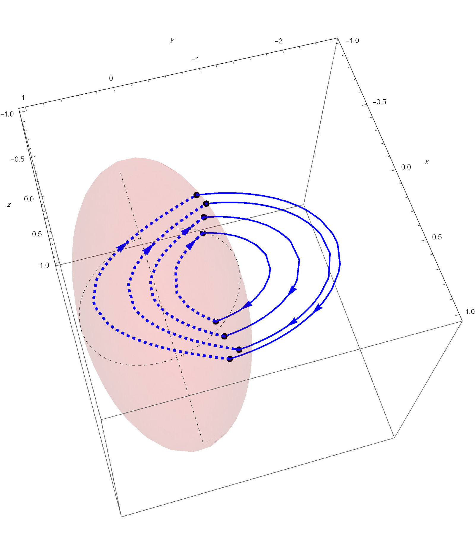
We recall that a point \(M_1\) (or \(N_1\)) is of a crossing type if the vector fields (2) and (3) move in the same direction with respect to the switching manifold \(\mathbb{S}^2\), this can be verified via the scalar product. The proof for the points \(M_1\) and \(N_1\) is summarized as follows: \[\begin{aligned} X^{+}(M_1) X^{-}(M_1)=& (-0.892664, -0.585185, -0.179271) (0.00840453, -0.180831, 0.0920966)\\ =&0.0818071.\\ X^{+}(N_1)X^{-}(N_1)=&(-1.27131, -0.0433098, 0.0607244)(-0.0426181, 0.170894, -0.0939709)\\ =&0.0410731. \end{aligned}\]
With \(X^{+}\equiv \text{(2)}\) and \(X^{-}\equiv \text{(3)}\). This establishes the unique three-dimensional crossing limit cycle for the discontinuous piecewise differential system (2)–(3), see Figure 1.
Now in the region \(\mathcal{R}_1\) we introduce system (2), defined by the parameters \[\begin{aligned} &(\alpha_{1},\alpha_{2},\alpha_{3},\alpha_{4},\beta_{1},\beta_{2},\beta_{3},\beta_{4}, \mu_{1},\mu_{2},\mu_{3},\mu_{4},\gamma_1, \lambda_1) \\ &\qquad\longrightarrow \bigg(7,6,6,\dfrac{3}{2},\dfrac{9}{2},-\dfrac{13}{10},\dfrac{53}{10},\dfrac{11}{5},\dfrac{2}{5},-1,-2,\dfrac{1}{5},\dfrac{374}{25},\dfrac{1521}{100}\bigg). \end{aligned}\]
In the region \(\mathcal{R}_2\) we have the parameters that characterize system (3) \[\begin{aligned} &\left(a_{1},a_{2},a_{3},a_{4},b_{1},b_{2},b_3,b_4, c_{1},c_2,c_3,c_4 , \gamma_2, \lambda_2\right)\\ &\qquad\longrightarrow \bigg(\dfrac{31}{5},9,2,7,\dfrac{7}{2},2,\dfrac{173881}{12138},\dfrac{54309}{26828},-\dfrac{4}{25},\dfrac{2}{5},\dfrac{4}{5},2,14,15\bigg). \end{aligned}\]
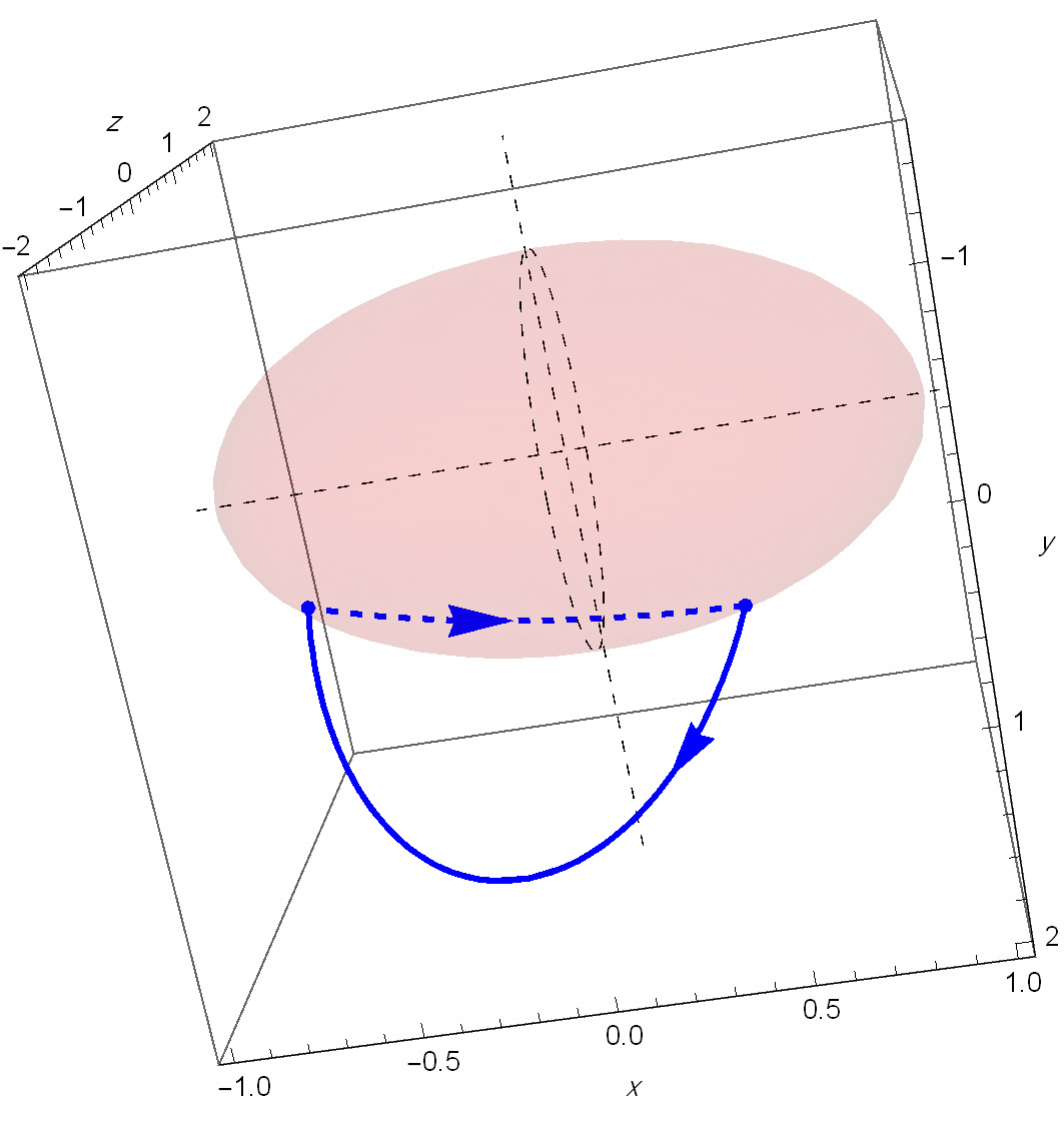
According to these systems, the two solutions fulfill system (4) are given by \[\begin{aligned} (M_1, N_1)=& (x_1, y_1, z_1, x_{11}, y_{11}, z_{11})\\ =&\left(-\dfrac{314449}{364284},\dfrac{58309}{203634},-\dfrac{110011}{264570},\dfrac{69597}{231377},-\dfrac{255470}{294203},\dfrac{131253}{332849} \right),\\ (M_2, N_2)=& (x_2, y_2, z_2, x_{22}, y_{22}, z_{22})\\ =&\left(-\dfrac{75659}{178994},\dfrac{68959}{212955},-\dfrac{186712}{220583},\dfrac{203569}{229776},\dfrac{12947}{182306},-\dfrac{125015}{272768}\right), \end{aligned}\] \(M_i\) and \(N_i\) with \(i=1,2\) are crossing points because we have \[\begin{aligned} X^{+}(M_1) X^{-}(M_1)=& (-1.35744, -0.4115, -0.0657385) (-0.00177526, -0.137162, 0.0682259)\\ =&0.05436.\\ X^{+}(N_1)X^{-}(N_1)=&(0.482879, 1.27907, -0.542961)(0.0498604, 0.0894612, -0.0347585)\\ =&0.1573.\\ X^{+}(M_2) X^{-}(M_2)=& (-1.81072, -0.583444, -0.0704217) (-0.0315458, -0.45152, 0.219451)\\ =&0.3051.\\ X^{+}(N_2)X^{-}(N_2)=&(-1.86752, 1.294, -1.02051)(-0.011807, 0.459895, -0.232309)\\ =&0.854228. \end{aligned}\]
Consequently, the discontinuous piecewise differential system (2)–(3) has two crossing limit cycles, illustrated in Figure 2.
Similarly, in the region \(\mathcal{R}_1\) we consider \[\begin{aligned} &(\alpha_{1},\alpha_{2},\alpha_{3},\alpha_{4},\beta_{1},\beta_{2},\beta_{3},\beta_{4}, \mu_{1},\mu_{2},\mu_{3},\mu_{4},\gamma_1, \lambda_1)\\ &\qquad\longrightarrow \bigg(15,4,-7,2,4,-1,5,2,\dfrac{1}{5},-1,-2,\dfrac{7333}{10000},\dfrac{149}{10},\dfrac{76}{5}\bigg), \end{aligned}\] to obtain the Euler system in the form (2).
For system (3) in the region \(\mathcal{R}_2\) we consider the parameters \[\begin{aligned} & \left(a_{1},a_{2},a_{3},a_{4},b_{1},b_{2},b_3,b_4, c_{1},c_2,c_3,c_4 , \gamma_2, \lambda_2\right)\\ &\longrightarrow \bigg(\dfrac{161641}{8574},4,-\dfrac{433567}{42472},7,\dfrac{7}{2},2,\dfrac{31}{5},-\dfrac{468626}{26985},-\dfrac{1}{5},1,2,2,14,15\bigg). \end{aligned}\]
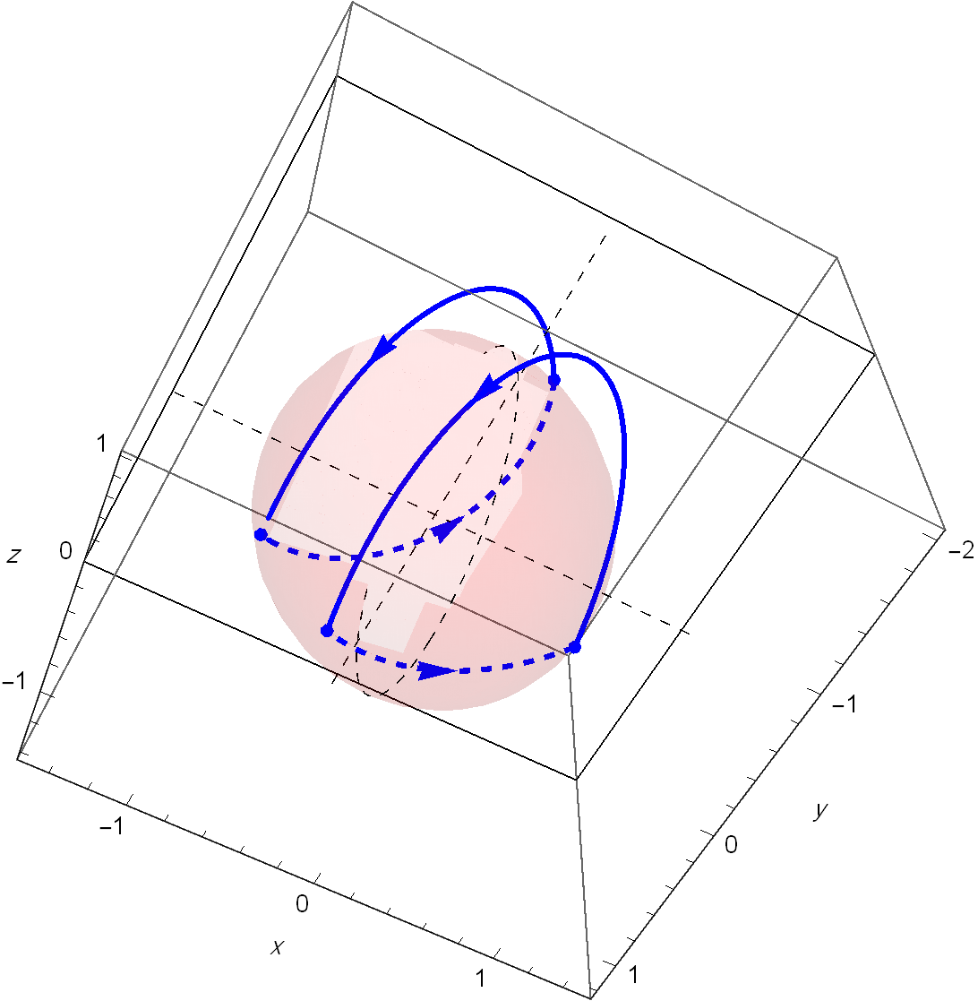
In this case, system (4) has three solutions \[\begin{aligned} (M_1,N_1)=&(x_1, y_1, z_1, x_{11}, y_{11}, \\ z_{11})=&\left(-\dfrac{1526}{3373},-\dfrac{19862}{23087},\dfrac{6287}{26763},\dfrac{20969}{30956},-\dfrac{74912}{108951},\dfrac{12253}{46852}\right),\\ (M_2,N_2)=&(x_2, y_2, z_2, x_{22}, y_{22}, \\ z_{22})=&\left(-\dfrac{14371}{29650},-\dfrac{17362}{19851},-\dfrac{172}{15411},\dfrac{20401}{35695},-\dfrac{10367}{12675},\dfrac{1697}{25670}\right),\\ (M_3,N_3)=& (x_3, y_3, z_3, x_{33}, y_{33}, \\ z_{33})=&\left(-\dfrac{21220}{48317},-\dfrac{40377}{45593},-\dfrac{3906}{25847},\dfrac{28112}{62799},-\dfrac{33331}{37356},-\dfrac{1879}{31789}\right), \end{aligned}\] where \[\begin{aligned} X^{+}(M_1) X^{-}(M_1)=& (0.302693, -0.485162, 0.27285) (1.36742,3.26975, -6,26602)\\ =&4.3461.\\ X^{+}(N_1)X^{-}(N_1)=&(-0.123483, 0.512562, -0.268629)(-4.37086, 5.80682, -3.3405)\\ =&4.41344.\\ X^{+}(M_2) X^{-}(M_2)=& (0.37469, -0.660432, 0.367685) (0.573592, -3.87574, 1.99523)\\ =&3.5082.\\ X^{+}(N_2)X^{-}(N_2)=&(-0.177128, 0.671039, -0.353232)(-3.02808, 3.74396, -2.17479)\\ =&3.81691.\\ X^{+}(M_3) X^{-}(M_3)=& (0.356697, -0.652729, 0.362034) (0.0958458, -2.32415, 1.17166)\\ =&1.97541.\\ X^{+}(N_3)X^{-}(N_3)=&(-0.172877, 0.65135, -0.342963)(-2.1003, 2.33919, -1.37963)\\ =&2.35989. \end{aligned}\]
Which yield three crossing limit cycles for the discontinuous piecewise differential system (2)–(3), as shown in Figure 3.
For the last example of piecewise differential system that exhibits four crossing limit cycles, we define the first Euler system in the region \(\mathcal{R}_1\) by the following parameters \[\begin{aligned} &(\alpha_{1},\alpha_{2},\alpha_{3},\alpha_{4},\beta_{1},\beta_{2},\beta_{3},\beta_{4}, \mu_{1},\mu_{2},\mu_{3},\mu_{4},\gamma_1, \lambda_1)\\ &\qquad\longrightarrow \bigg(14,-\dfrac{1}{5},8,1,2,5,\dfrac{4}{5},3,-3,\dfrac{3}{10},3,1,\dfrac{72}{5},18\bigg). \end{aligned}\]
We proceed by considering the following parameters for the second Euler system in the region \(\mathcal{R}_2\) \[\begin{aligned} & \left(a_{1},a_{2},a_{3},a_{4},b_{1},b_{2},b_3,b_4, c_{1},c_2,c_3,c_4 , \gamma_2, \lambda_2\right)\\ &\longrightarrow \bigg(15,\dfrac{9}{20},\dfrac{148217}{19381},-\dfrac{28633}{30950},-\dfrac{100454}{78393},-1,-\dfrac{1}{2}, -\dfrac{1322481}{40118},-1,\dfrac{1}{10},1,\dfrac{333}{1000},\dfrac{147}{10},-\dfrac{76}{5}\bigg). \end{aligned}\]
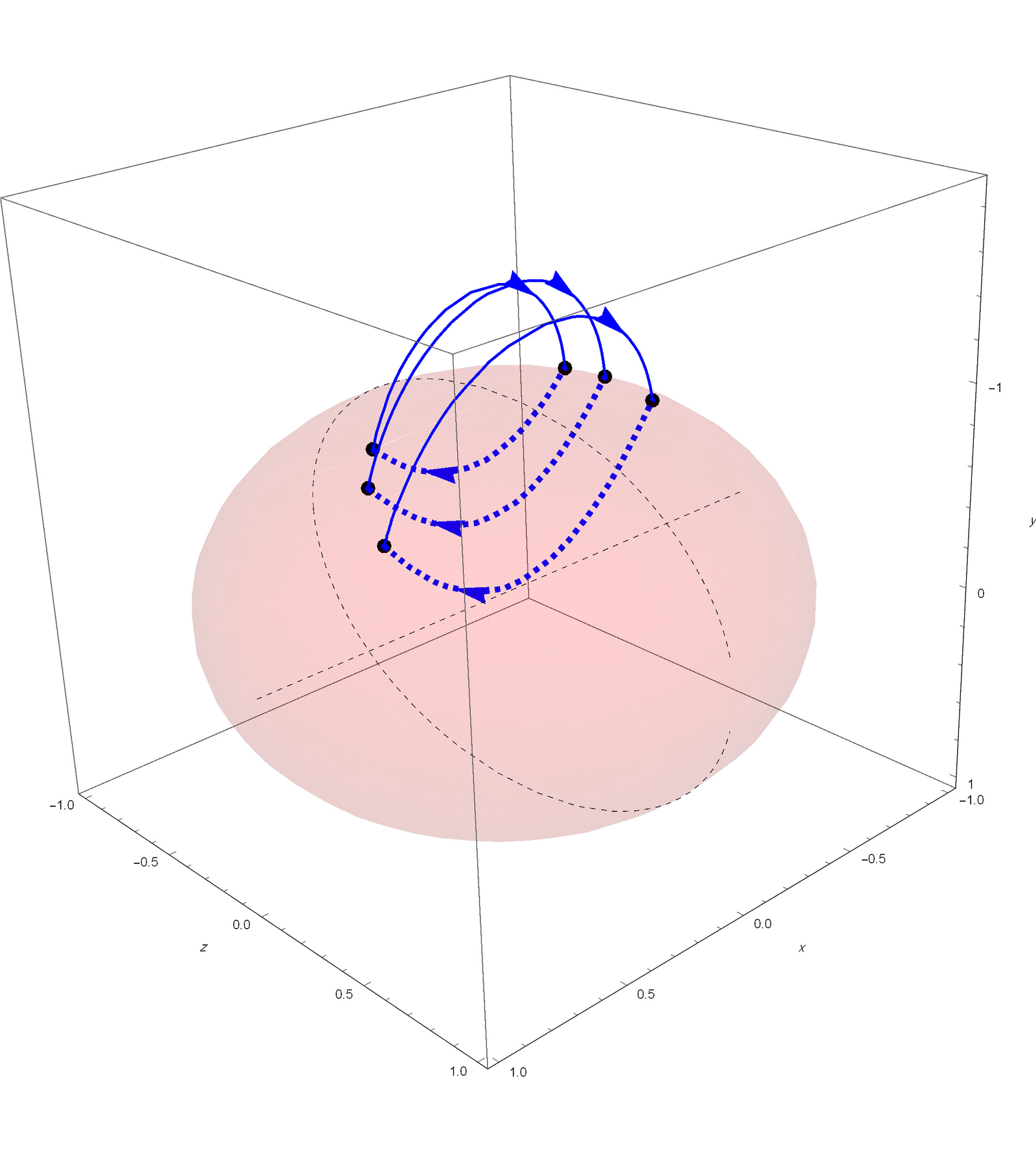
System (4) has the four solutions \[\begin{aligned} (M_1,N_1)=& (x_1, y_1, z_1, x_{11}, y_{11}, z_{11})\\ =&\left(-\dfrac{18238}{33481},-\dfrac{26557}{32345},\dfrac{5465}{32013},-\dfrac{3599}{58910},-\dfrac{20733}{27314},\dfrac{31940}{49279}\right),\\ (M_2,N_2)=& (x_2, y_2, z_2, x_{22}, y_{22}, z_{22})\\ =&\left(-\dfrac{19973}{33629},-\dfrac{23384}{31087},-\dfrac{5759}{20181},\dfrac{7857}{28507},-\dfrac{24157}{31677},\dfrac{13849}{23665}\right), \\ (M_3,N_3)= & (x_3, y_3, z_3, x_{33}, y_{33}, z_{33})\\ =&\left(-\dfrac{23451}{42434},-\dfrac{15915}{19114},-\dfrac{937}{25992},\dfrac{2119}{23702},-\dfrac{31217}{39345},\dfrac{12466}{20705}\right), \\ (M_4,N_4)=& (x_4, y_4, z_4, x_{44}, y_{44}, z_{44})\\ =&\left(-\dfrac{16360}{34739},-\dfrac{18796}{23299},-\dfrac{9649}{27033},\dfrac{21157}{72139},-\dfrac{36224}{42009},\dfrac{14137}{34243}\right), \end{aligned}\] that satisfy the crossing condition: \[\begin{aligned} X^{+}(M_1) X^{-}(M_1)=& (-0.472908, 11.0832, -1.58122) (42.5667, 168.359, 25.7308)\\=&1805.13.\\ X^{+}(N_1)X^{-}(N_1)=&(-0.699946, -11.2335, 0.423405)(39.2069, -157.877, 54.9946)\\=&1769.35.\\ X^{+}(M_2) X^{-}(M_2)=& (-0.0696876, 11.7913, -1.24882) (25.7976, 171.845, 8.61315)\\=&2013.72.\\ X^{+}(N_2)X^{-}(N_2)=&(-0.478259, -11.7848, 0.700217)(22.1639, -172.418, 39.4057)\\=&2048.9.\\ X^{+}(M_3) X^{-}(M_3)=& (-0.331368, 11.7316, -1.50453) (34.1904, 173.829, 16.8075)\\=&2002.69.\\ X^{+}(N_3)X^{-}(N_3)=&(-0.651386, -11.7917, 0.527781)(30.6086, -169.871, 47.5957)\\=&2008.25.\\ X^{+}(M_4) X^{-}(M_4)=& (-0.101183, 6.72784, -0.773967) (16.5201, 96.7951, 6.84064)\\=&644.256.\\ X^{+}(N_4)X^{-}(N_4)=&(-0.375268, -6.6932, 0.294052)(14.4313, -6.6932, 0.294052)\\=&39.4699, \end{aligned}\] which provides the existence of four crossing limit cycles for the discontinuous piecewise differential system (2)–(3) separated by the unit sphere \(\mathbb{S}^2\). See Figure 4.