
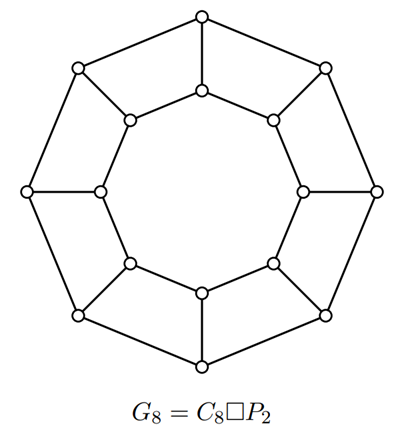
We study the prism (cyclic ladder) family \(G_n=C_n\square P_2\), a fixed-width cyclic strip graph (see Figure 1). Its chromatic polynomial admits the finite spectral expansion \[ P(G_n,z)=\sum\limits_{j=0}^3 \alpha_j(z)\lambda_j(z)^n,\tag{1}\] where \[ \lambda_0=z^2-3z+3,\quad \lambda_1=1-z,\quad \lambda_2=3-z,\quad \lambda_3=1,\tag{2}\] and \[ \alpha_0=1,\quad \alpha_1=z-1,\quad \alpha_2=z-1,\quad \alpha_3=1+z(z-3).\tag{3}\]
Each \(\lambda_j\) and \(\alpha_j\) is a polynomial in \(z\), hence entire.
The complete algebraic classification of all equimodular tie curves for the prism family, including explicit quartic equations for the quadratic-linear balances, is established in [1]. The present paper has a different objective: it extracts a geometric normal form for the dominant ties and proves a uniform finite-\(n\) containment theorem via a global Rouché comparison.
Under the Beraha-Kahane-Weiss (BKW) mechanism [3], isolated accumulation points can arise only at zeros of an amplitude \(\alpha_j\) for which \(\lambda_j\) is dominant. From (3), amplitude zeros occur at \(z=1\) and \(z_\pm=\frac{3\pm\sqrt5}{2}\). At each of these points the vanishing branch is strictly non-dominant, so no isolated amplitude-zero BKW limit points occur; all candidates arise from dominant equimodular ties.
For fixed-width strip graphs, BKW theory determines the asymptotic root skeleton through equimodularity of competing branches [3, 7, 4]. What it does not provide is a uniform exclusion region valid for every finite \(n\). Here a global Rouché comparison yields such a result: all chromatic roots of \(G_n\) lie in \(\left|z\right|<6\) for every \(n\ge3\) (Theorem 3.5).
The principal quadratic-linear ties \[ \mathcal{C}_{01}:\ \left|z^2-3z+3\right|=\left|1-z\right|, \qquad \mathcal{C}_{02}:\ \left|z^2-3z+3\right|=\left|3-z\right|,\tag{4}\] govern the outer envelope of the BKW skeleton. After translating \(w=z-\tfrac32\), the quadratic factorizes symmetrically as \[\lambda_0=w^2+\tfrac34=\left(w-\mathrm{i}\tfrac{\sqrt3}{2}\right)\left(w+\mathrm{i}\tfrac{\sqrt3}{2}\right),\] so the ties assume a centered Cassini-type product-of-distances form. This normalization clarifies their quartic structure and interfaces directly with the dominance arguments underlying the uniform Rouché bound.
The paper thus separates asymptotic BKW geometry from finite-\(n\) analytic control, combining explicit equimodular structure with certified global containment in a fixed strip family.
Rather than viewing the principal modulus-tie sets solely through their defining algebraic equations, we adopt a geometric perspective that exposes their underlying structure. In the BKW mechanism, equimodular loci arise precisely from comparisons of competing analytic terms; in the prism family, this comparison has a classical interpretation in terms of product-of-distances geometry. Here the eigenvalues \(\lambda_j\) and amplitudes \(\alpha_j\) are polynomials, hence analytic on \(\mathbb{C}\), so the BKW framework applies without singularity issues. We recall the relevant notion and then show that it emerges naturally from the centered eigenvalue expansion of \(P(G_n,z)\).
A Cassini oval is the planar locus of points whose product of distances to two fixed foci is constant: given distinct points \(F_1,F_2\in\mathbb{C}\) and \(c>0\), it is the set \[\mathcal{K}(F_1,F_2;c) = \bigl\{z\in\mathbb{C}:\ \left|z-F_1\right|\,\left|z-F_2\right|=c\bigr\}.\]
More generally, we call any level set of the form \[\left|z-F_1\right|\,\left|z-F_2\right|=\left|z-F_3\right|,\] with fixed \(F_1,F_2,F_3\in\mathbb{C}\), a Cassini-type curve. Such loci retain the characteristic two-lobed geometry of classical Cassini ovals and occur naturally in root-locus problems when equating moduli of polynomial or exponential terms [6, 9]. In the present setting, this framework provides a transparent geometric explanation for the principal BKW tie sets (4), clarifying both their quartic nature and their role in shaping the asymptotic outer envelope of chromatic roots analyzed in later sections.
Proposition 2.1 (Centered factorization). Define \(w=z-\tfrac{3}{2}\) and let \(a=\tfrac{\sqrt{3}}{2}\). Then \[\begin{aligned} \lambda_0(z) &= w^2+a^2=(w-\mathrm{i}a)(w+\mathrm{i}a),\\ \lambda_1(z) &= -\left(w+\tfrac{1}{2}\right),\\ \lambda_2(z) &= -\left(w-\tfrac{3}{2}\right),\\ \lambda_3(z) &= 1. \end{aligned}\]
Consequently, the tie sets (4) take the centered form \[ \mathcal{C}_{01}:\ \left|w-\mathrm{i}a\right|\,\left|w+\mathrm{i}a\right|=\left|w+\tfrac{1}{2}\right|, \qquad \mathcal{C}_{02}:\ \left|w-\mathrm{i}a\right|\,\left|w+\mathrm{i}a\right|=\left|w-\tfrac{3}{2}\right|.\tag{5}\]
Proof. Completing the square yields \[z^2-3z+3=\left(z-\tfrac{3}{2}\right)^2+\tfrac{3}{4}=w^2+a^2,\] with \(a^2=3/4\). The linear identities follow from \(1-z=-\left(w+\tfrac12\right)\) and \(3-z=-\left(w-\tfrac32\right)\). Taking absolute values removes the minus signs and gives (5). \(\square\)
Remark 2.2 (Cassini-type geometry). In the centered coordinate \(w=z-\tfrac{3}{2}\), each equation in (5) equates the product of distances to the conjugate foci \(\pm \mathrm{i}a\) with the distance to a third real focus (\(-1/2\) or \(3/2\), respectively). The centering at \(z=\tfrac32\) is canonical in the elementary sense that it moves the quadratic \(\lambda_0\) to its vertex, so that \(\lambda_0=w^2+a^2\) factors symmetrically with no additional structure imposed beyond this normalization. Thus the principal tie sets \(\mathcal{C}_{01}\) and \(\mathcal{C}_{02}\) are Cassini-type product-of-distances loci. Such quadratic-linear equimodularity is a general phenomenon; what is specific here is the explicit identification of the resulting Cassini geometry for the prism family. This geometric viewpoint explains their characteristic two-lobed appearance in numerical plots and provides a conceptual complement to the explicit quartic equations derived in [1].
While the Cassini interpretation provides geometric intuition, it is often convenient to work with explicit analytic representations. We therefore record equivalent real-algebraic quartic equations and centered polar forms for the principal tie curves, which will be used both for dominance analysis and for comparison with numerical root data.
Proposition 2.3 (Quartic implicit equations). Write \(z=x+\mathrm{i}y\) and define \[ A(x,y)=x^2-y^2-3x+3, \qquad B(x,y)=2xy-3y.\tag{6}\]
Then \[\left|\lambda_0(z)\right|^2=A(x,y)^2+B(x,y)^2,\qquad \left|\lambda_1(z)\right|^2=(1-x)^2+y^2,\qquad \left|\lambda_2(z)\right|^2=(3-x)^2+y^2.\]
Consequently, \(\mathcal{C}_{01}\) and \(\mathcal{C}_{02}\) are the real-algebraic quartic curves \[\mathcal{C}_{01}:\quad F_{01}(x,y):=A(x,y)^2+B(x,y)^2-\bigl((1-x)^2+y^2\bigr)=0.\tag{7}\] \[\mathcal{C}_{02}:\quad F_{02}(x,y):=A(x,y)^2+B(x,y)^2-\bigl((3-x)^2+y^2\bigr)=0.\tag{8}\]
These formulas are derived directly from the eigenvalue expressions (2) and are self-contained; no external classification is required for their validity.
Proof. A direct expansion gives \[\lambda_0(z)=(x+\mathrm{i}y)^2-3(x+\mathrm{i}y)+3=\bigl(x^2-y^2-3x+3\bigr)+\mathrm{i}(2xy-3y)=A(x,y)+\mathrm{i}B(x,y),\] hence \(\left|\lambda_0(z)\right|^2=A^2+B^2\). The remaining identities are standard. Substituting into (4) yields (7)–(8). \(\square\)
Proposition 2.4 (Centered polar equations). Let \(w=\rho\mathrm{e}^{\mathrm{i}\theta}\) with \(\rho\ge 0\) and \(\theta\in\mathbb{R}\), where \(w=z-\tfrac{3}{2}\) and \(a=\tfrac{\sqrt{3}}{2}\). Then \[\begin{aligned} \left|\lambda_0(z)\right|^2 &= \rho^4+\tfrac{3}{2}\rho^2\cos(2\theta)+\tfrac{9}{16},\\ \left|\lambda_1(z)\right|^2 &= \rho^2+\rho\cos\theta+\tfrac{1}{4},\\ \left|\lambda_2(z)\right|^2 &= \rho^2-3\rho\cos\theta+\tfrac{9}{4}. \end{aligned}\]
Consequently, \(\mathcal{C}_{01}\) and \(\mathcal{C}_{02}\) satisfy \[\mathcal{C}_{01}:\quad \rho^4+\tfrac{3}{2}\rho^2\cos(2\theta)+\tfrac{9}{16}=\rho^2+\rho\cos\theta+\tfrac{1}{4}.\tag{9}\] \[\mathcal{C}_{02}:\quad \rho^4+\tfrac{3}{2}\rho^2\cos(2\theta)+\tfrac{9}{16}=\rho^2-3\rho\cos\theta+\tfrac{9}{4}.\tag{10}\]
For each fixed \(\theta\), these reduce to quartic equations in \(\rho\) whose positive real solutions trace the curves.
Proof. Using \(\lambda_0(z)=w^2+a^2\) and \(w=\rho\mathrm{e}^{\mathrm{i}\theta}\) gives \[\left|\lambda_0(z)\right|^2=\left|\rho^2\mathrm{e}^{2\mathrm{i}\theta}+a^2\right|^2 =\rho^4+2a^2\rho^2\cos(2\theta)+a^4.\]
The formulas for \(\left|\lambda_1(z)\right|^2\) and \(\left|\lambda_2(z)\right|^2\) follow by expanding \(\left|w+c\right|^2=\rho^2+2c\rho\cos\theta+c^2\) with \(c=\tfrac12\) and \(c=-\tfrac32\). Substituting into (4) yields (9)–(10). \(\square\)
These representations make explicit that the tie curves are compact real-algebraic sets, a fact exploited in the dominance and exclusion arguments of the next subsection and in the global bounds established in Section 3.
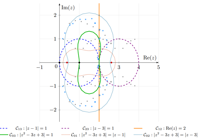
For \(0\le i<j\le 3\), define the equimodular tie sets \[ \mathcal{C}_{ij} := \{\,z\in\mathbb{C}:\ |\lambda_i(z)|=|\lambda_j(z)|\,\}.\tag{11}\] For the prism branches \[\lambda_0(z)=z^2-3z+3,\quad \lambda_1(z)=1-z,\quad \lambda_2(z)=3-z,\quad \lambda_3(z)=1,\] the elementary ties (instances of (11)) are \[\begin{aligned} \mathcal{C}_{12}&=\{z\in\mathbb{C}:\ \mathop{\mathrm{Re}}(z)=2\},\\ \mathcal{C}_{13}&=\{z\in\mathbb{C}:\ |z-1|=1\},\\ \mathcal{C}_{23}&=\{z\in\mathbb{C}:\ |z-3|=1\},\\ \mathcal{C}_{03}&=\{z\in\mathbb{C}:\ |z^2-3z+3|=1\}, \end{aligned}\] while the quadratic–linear ties are \[\mathcal{C}_{01}=\{z\in\mathbb{C}:\ |z^2-3z+3|=|z-1|\}, \qquad \mathcal{C}_{02}=\{z\in\mathbb{C}:\ |z^2-3z+3|=|z-3|\}.\]
The sets \(\mathcal{C}_{01}\) and \(\mathcal{C}_{02}\) describe where moduli coincide, but not every such point contributes to root accumulation. To isolate the portion of the BKW skeleton that governs the outer envelope, dominance conditions must be imposed.
Definition 2.5 (Dominance-trimmed envelope arcs). Define \[\mathcal{C}_{01}^*:=\bigl\{z\in\mathbb{C}:\ |\lambda_0(z)|=|\lambda_1(z)|\ge\max\{|\lambda_2(z)|,|\lambda_3(z)|\}\bigr\}.\tag{12}\] \[\mathcal{C}_{02}^*:=\bigl\{z\in\mathbb{C}:\ |\lambda_0(z)|=|\lambda_2(z)|\ge\max\{|\lambda_1(z)|,|\lambda_3(z)|\}\bigr\}.\tag{13}\]
These sets consist precisely of the equimodular points at which the tied branches dominate all others.
To establish compactness of these dominance-trimmed arcs, we first prove radius bounds for the full equimodular sets.
Theorem 2.6 (Radius bounds for quadratic ties). Let \(z\in\mathbb{C}\) and set \(r=|z|\). Then:
(a) If \(|\lambda_0(z)|=|\lambda_1(z)|\), then \(r\le 2+2\sqrt2\).
(b) If \(|\lambda_0(z)|=|\lambda_2(z)|\), then \(r\le 2+\sqrt{10}\).
(c) If \(|\lambda_0(z)|=1\), then \(r\le 4\).
Consequently, \[\mathcal{C}_{01}\cup\mathcal{C}_{02}\subseteq\{\,|z|\le 2+\sqrt{10}\,\}.\]
Proof. For all \(z\in\mathbb{C}\) we have the reverse triangle estimate \[ |\lambda_0(z)|=|z^2-3z+3|\ge r^2-3r-3.\tag{14}\]
(a) If \(|\lambda_0(z)|=|\lambda_1(z)|\), then \(|z^2-3z+3|=|1-z|\le r+1\), so (14) yields \(r^2-3r-3\le r+1\), i.e., \(r^2-4r-4\le0\), hence \(r\le2+2\sqrt2\).
(b) If \(|\lambda_0(z)|=|\lambda_2(z)|\), then \(|z^2-3z+3|=|3-z|\le r+3\), so (14) yields \(r^2-3r-3\le r+3\), i.e., \(r^2-4r-6\le0\), hence \(r\le2+\sqrt{10}\).
(c) If \(|\lambda_0(z)|=1\), then (14) gives \(r^2-3r-3\le1\), i.e., \(r^2-3r-4\le0\), hence \(r\le4\).
Since \(2+2\sqrt2<2+\sqrt{10}\), the claimed containment follows. \(\square\)
Proposition 2.7 (Local smoothness). For \(j\in\{1,2\}\), the set \(\mathcal{C}_{0j}^*\) is semialgebraic in \(\mathbb{R}^2\simeq\mathbb{C}\) and has (real) dimension at most \(1\). Moreover, every point of \(\mathcal{C}_{0j}^*\) has a neighborhood in which \(\mathcal{C}_{0j}^*\) is contained in a finite union of real–analytic arcs. A point \(z\in\mathcal{C}_{0j}^*\) can fail to be locally a single real–analytic arc only if
(i) \(z\) is a singular point of the algebraic curve \(\mathcal{C}_{0j}\),
(ii) \(z\) lies on an intersection \(\mathcal{C}_{0j}\cap \mathcal{C}_{ik}\) with some \((i,k)\neq(0,j)\), or
(iii) at \(z\) at least one dominance inequality in (12)–(13) is tight.
Proof. Write \(z=x+\mathrm{i}y\). For \(j\in\{1,2\}\) let \(F_{0j}\in\mathbb{R}[x,y]\) be the defining quartic from (7)–(8), so \(\mathcal{C}_{0j}=\{(x,y):F_{0j}(x,y)=0\}\). Each dominance constraint in (12)–(13) can be written as a weak polynomial inequality after squaring moduli (e.g. \(|\lambda_a|^2-|\lambda_b|^2\ge0\)), hence the dominance region \(D_j\subseteq\mathbb{R}^2\) is semialgebraic and \[\mathcal{C}_{0j}^*=\mathcal{C}_{0j}\cap D_j,\] is semialgebraic. Since \(\mathcal{C}_{0j}\subseteq\mathbb{R}^2\) is an algebraic curve, \(\dim(\mathcal{C}_{0j})\le1\), and thus \(\dim(\mathcal{C}_{0j}^*)\le1\).
Fix \(p=(x_0,y_0)\in\mathcal{C}_{0j}^*\). If \(\nabla F_{0j}(p)\neq0\), then by the Implicit Function Theorem the germ of \(\mathcal{C}_{0j}\) at \(p\) is a single real–analytic arc. If, in addition, \(p\) satisfies all dominance inequalities strictly and lies on no other tie curve, then these strict inequalities persist on a neighborhood of \(p\) (by continuity), so \(\mathcal{C}_{0j}^*\) coincides locally with that same single arc. Hence, failure of local uniqueness at a regular point forces either membership in another tie curve (ii) or tightness of a dominance inequality (iii).
If \(\nabla F_{0j}(p)=0\), then \(p\) is a singular point of the real algebraic curve \(\mathcal{C}_{0j}\), and the standard local structure of real algebraic plane curves implies that the germ of \(\mathcal{C}_{0j}\) at \(p\) is a finite union of real–analytic arcs; intersecting with \(D_j\) preserves finiteness. This is case (i). \(\square\)
Proposition 2.8 (Global structural properties). For \(j\in\{1,2\}\), the set \(\mathcal{C}_{0j}^*\) is compact and contained in the disk \(|z|\le 2+\sqrt{10}\). Moreover:
(i) \(\mathcal{C}_{0j}^*\) is a finite union of closed real–analytic arcs. Each endpoint occurs only at
(a) an intersection with another tie curve \(\mathcal{C}_{ik}\),
(b) a singular point of the algebraic curve \(\mathcal{C}_{0j}\), or
(c) a boundary point where at least one dominance inequality is tight.
(ii) Every BKW accumulation point of chromatic roots of \(G_n\) lying on \(\mathcal{C}_{0j}\) belongs to \(\mathcal{C}_{0j}^*\).
Proof. Compactness and radius bound. By definition \(\mathcal{C}_{0j}^*\subseteq\mathcal{C}_{0j}\). Theorem 2.6 gives \(\mathcal{C}_{01}\subseteq\{|z|\le 2+2\sqrt2\}\) and \(\mathcal{C}_{02}\subseteq\{|z|\le 2+\sqrt{10}\}\), hence \(\mathcal{C}_{0j}^*\subseteq\{|z|\le 2+\sqrt{10}\}\). Also \(\mathcal{C}_{0j}^*=\mathcal{C}_{0j}\cap D_j\) with \(D_j\) defined by weak inequalities in continuous functions, so \(D_j\) is closed, and \(\mathcal{C}_{0j}\) is closed as a zero set. Thus \(\mathcal{C}_{0j}^*\) is closed; being closed and bounded, it is compact.
Finite union of arcs and endpoint types. Since \(\mathcal{C}_{0j}^*\) is compact semialgebraic, it has finitely many connected components and admits a finite semialgebraic stratification into \(0\)– and \(1\)-dimensional real–analytic strata (e.g. [2]). Each \(1\)-dimensional stratum is a real–analytic embedded \(1\)-manifold, hence a finite union of real–analytic arcs; compactness makes each such arc closed. This proves (i) up to the endpoint classification.
Let \(\gamma\) be one such arc and let \(z\in\gamma\) be an endpoint. If \(z\) were a regular point of \(\mathcal{C}_{0j}\), lay on no other tie curve, and satisfied all dominance inequalities strictly, then by Proposition 2.7 the set \(\mathcal{C}_{0j}^*\) would contain a two-sided neighborhood of \(z\) along the analytic arc of \(\mathcal{C}_{0j}\) through \(z\), contradicting that \(z\) is an endpoint. Hence at any endpoint at least one of (a)–(c) must occur.
BKW trimming. In the expansion (1), all \(\lambda_i\) and \(\alpha_i\) are entire. By the BKW theorem, any accumulation point arising from a tie \(\mathcal{C}_{0j}\) must occur where the tied moduli \(|\lambda_0|\) and \(|\lambda_j|\) are weakly maximal among all branches with nonvanishing amplitude at that point (i.e., the tied pair achieves \(\max_k |\lambda_k(z)|\)). Indeed, if some \(k \notin \{0,j\}\) satisfies \(|\lambda_k(z)| > \max\{|\lambda_0(z)|, |\lambda_j(z)|\}\) and \(\alpha_k(z) \neq 0\), then the \(k\)-th term dominates in a neighborhood and prevents accumulation on the \(\{0,j\}\)-tie. This weak maximality condition is precisely the dominance requirement in (12)–(13), so such accumulation points lie in \(\mathcal{C}_{0j}^*\), proving (ii). \(\square\)
Figure 2 displays the equimodular sets \(\mathcal{C}_{ij}\) together with representative finite-\(n\) chromatic roots. It illustrates the asymptotic BKW skeleton; no finite-\(n\) outer-envelope statement is implied beyond the uniform containment theorem proved in Section 3.
The preceding sections identify the geometric skeleton along which chromatic roots may accumulate asymptotically, as dictated by the BKW theorem. By its nature, however, BKW theory is asymptotic and does not furnish quantitative exclusion regions for any fixed graph in the family. For fixed-width strip families admitting a finite-branch expansion such as (1), this gap can be closed by combining BKW geometry with analytic comparison arguments of Rouché type. The resulting synthesis yields both a precise description of limiting root geometry and certified uniform containment for every finite \(n\).
From (1), the chromatic polynomial of the prism family admits the explicit closed form \[ P(G_n,z) = \bigl(z^2-3z+3\bigr)^n +(z-1)(1-z)^n +(z-1)(3-z)^n +\bigl(1+z(z-3)\bigr),\tag{15}\] derived in full detail in [1]. This representation isolates the dominant exponential contributions and provides a natural starting point for non-asymptotic root exclusion via Rouché’s theorem.
For fixed-width strip families, chromatic polynomials take the general form \[P(G_n,z)=\sum\limits_{j=0}^{m-1}\alpha_j(z)\lambda_j(z)^n,\] where the number of branches \(m\) is constant, the eigenvalues \(\lambda_j\) are analytic, and the amplitudes \(\alpha_j\) are algebraic functions. In the prism family, all \(\lambda_j\) and \(\alpha_j\) are polynomials, hence analytic on \(\mathbb{C}\). This structure naturally separates two complementary tasks: identifying the asymptotic root geometry via BKW equimodularity, and certifying finite-\(n\) exclusion regions via analytic dominance.
Lemma 3.1 (Rouché dominance principle). Let \(\Gamma\) be a positively oriented simple closed contour and write \[f_n(z)=\alpha_k(z)\lambda_k(z)^n, \qquad g_n(z)=\sum\limits_{j\neq k}\alpha_j(z)\lambda_j(z)^n .\]
If \(\left|f_n(z)\right|>\left|g_n(z)\right|\) for all \(z\in\Gamma\), then \(P(G_n,z)=f_n(z)+g_n(z)\) and \(f_n(z)\) have the same number of zeros inside \(\Gamma\), counted with multiplicity. In particular, if \(f_n\) is zero-free on and inside \(\Gamma\) (equivalently, if \(\alpha_k\) and \(\lambda_k\) have no zeros in the enclosed region), then \(P(G_n,\cdot)\) is zero-free there.
Proof. This is an immediate application of Rouché’s theorem to \(f_n\) and \(g_n\) on \(\Gamma\). \(\square\)
Within this framework, BKW theory identifies the loci where dominance may fail (or amplitudes vanish), while Lemma 3.1 supplies the complementary finite-\(n\) certification: away from these loci, dominance implies zero-freeness.
We now apply this framework globally to the prism family \(G_n=C_n\square P_2\). Here \(\alpha_0\equiv 1\) and \(\lambda_0(z)=z^2-3z+3\), so exclusion reduces to establishing uniform modulus gaps on circles.
Lemma 3.2 (Sharp lower bound on a circle). Let \(R\ge 4\) and \(\left|z\right|=R\). Then \[\left|z^2-3z+3\right|\ \ge\ R^2-3R+3,\] with equality if and only if \(z=R\) (i.e., \(\theta=0\)).
Proof. Write \(z=Re^{\mathrm{i}\theta}\) and consider \[\phi(\theta):=\left|z^2-3z+3\right|^2 =\left|R^2e^{2\mathrm{i}\theta}-3Re^{\mathrm{i}\theta}+3\right|^2.\]
Expanding and collecting real parts gives \[\phi(\theta) = R^4+9R^2+9 -6R^3\cos\theta +6R^2\cos(2\theta) -18R\cos\theta .\]
Using \(\cos(2\theta)=2\cos^2\theta-1\) and writing \(u=\cos\theta\), this becomes a quadratic polynomial in \(u\): \[\phi(\theta)=a(R)u^2+b(R)u+c(R),\] where \[a(R)=12R^2,\qquad b(R)=-6R(R^2+3),\qquad c(R)=R^4+3R^2+9.\]
Since \(a(R)>0\), the quadratic is convex in \(u\). Its vertex occurs at \[u_0=-\frac{b(R)}{2a(R)} =\frac{R^2+3}{4R} =\frac14\left(R+\frac{3}{R}\right).\]
For \(R\ge 4\), we have \(u_0>1\), so the minimum of \(\phi(\theta)\) on \(u\in[-1,1]\) is attained at \(u=1\), i.e., at \(\theta=0\). Evaluating at \(\theta=0\) gives \[\phi(0)=(R^2-3R+3)^2.\]
Taking square roots yields the stated bound, and equality holds precisely at \(z=R\). \(\square\)
Lemma 3.3 (Elementary upper bounds). If \(\left|z\right|=R\), then \[\left|1-z\right|\le R+1,\qquad \left|3-z\right|\le R+3,\qquad \left|1+z(z-3)\right|\le R^2+3R+1.\]
Proof. Each inequality follows directly from the triangle inequality. \(\square\)
Lemma 3.4 (Monotone Rouché inequality). For every integer \(n\ge 3\), \[7^{n+1}+7\cdot 9^n+55 \;<\; 21^n .\]
Proof. Divide by \(21^n\) to write \[7\Bigl(\frac13\Bigr)^n + 7\Bigl(\frac{3}{7}\Bigr)^n + 55\cdot 21^{-n}.\]
Each term is strictly decreasing in \(n\). Hence it suffices to verify the inequality at \(n=3\): \[\frac{7}{27}+\frac{27}{49}+\frac{55}{9261}<1.\]
Multiplying by \(21^3\) yields \(7^4+7\cdot 9^3+55<21^3\), and the claim follows for all \(n\ge 3\). \(\square\)
Theorem 3.5 (Uniform disk bound). For every \(n\ge 3\), all chromatic roots of \(G_n\) lie in the disk \(\left|z\right|<6\).
Proof. Fix \(R=6\) and suppose \(|z|=6\). By Lemma 3.2, \[|\lambda_0(z)|=|z^2-3z+3|\ge 6^2-3\cdot6+3=21,\] hence \(|\lambda_0(z)^n|\ge 21^n\).
From Lemma 3.3 we have \[|(z-1)(1-z)^n|\le 7^{\,n+1},\qquad |(z-1)(3-z)^n|\le 7\cdot 9^n,\qquad |1+z(z-3)|\le 55.\]
Therefore the remainder term \[R_n(z):=(z-1)(1-z)^n+(z-1)(3-z)^n+1+z(z-3)\] satisfies \[|R_n(z)|\le 7^{\,n+1}+7\cdot9^n+55.\]
By Lemma 3.4, \[7^{\,n+1}+7\cdot9^n+55<21^n \quad\text{for every }n\ge3.\]
Hence on \(|z|=6\), we have \(|R_n(z)|<|\lambda_0(z)^n|\).
By Rouché’s theorem, \(P(G_n,\cdot)\) and \(\lambda_0(\cdot)^n\) have the same number of zeros in \(|z|<6\). The quadratic \(\lambda_0(z)=z^2-3z+3\) has two zeros \[z=\frac{3\pm \mathrm{i}\sqrt3}{2},\] both of modulus \(\sqrt3<6\). Thus \(\lambda_0(z)^n\) has exactly \(2n\) zeros in \(|z|<6\), counted with multiplicity. Since \(\deg P(G_n,z)=2n\), all zeros of \(P(G_n,z)\) lie in \(|z|<6\). \(\square\)
Remark 3.6. The constant \(6\) is not optimal; sharper estimates allow modest improvement. Reaching radii near \(2+\sqrt{10}\) would require exploiting argument information or a different comparison function.
The prism family admits an explicit constant-branch representation (1) and the certified containment disk of Theorem 3.5. We record two algorithmic consequences specific to such finite-branch strip families and then provide a numerical illustration of the BKW skeleton inside the certified region.
Recall the constant-branch expansion (1) with eigenvalues (2) and polynomial amplitudes (3). For a fixed complex number \(z\) of bounded precision, the quantities \(\lambda_j(z)\) and \(\alpha_j(z)\) are computed in constant time; the only growth with \(n\) arises from exponentiation.
Proposition 4.1 (Arithmetic complexity of point evaluation). Fix \(z\in\mathbb{C}\). The value \(P(G_n,z)\) can be computed using \(O(\log n)\) complex multiplications (and \(O(\log n)\) additions) by evaluating \(\lambda_j(z)^n\) via binary exponentiation for \(j=0,1,2\) and forming the linear combination.
Proof. Binary exponentiation computes \(w^n\) using at most \(2\lfloor \log_2 n\rfloor+O(1)\) multiplications. Since the number of branches is constant, assembling the four terms adds only \(O(1)\) arithmetic operations. \(\square\)
For coefficient-level computations, view \(P(G_n,z)\) as a degree-\(2n\) polynomial in \(z\). Because the expansion (1) has four fixed branches, the sequence \(\{P(G_n,z)\}_{n\ge1}\) satisfies a linear recurrence of order at most \(4\) with polynomial coefficients in \(z\), equivalently a constant-size linear representation. Thus coefficient extraction is polynomial-time in \(n\), in contrast with general graphs.
Proposition 4.2 (Arithmetic complexity for coefficient extraction). Let \(P(G_n,z)=\sum\limits_{k=0}^{2n} c_{n,k} z^k\). All coefficients \((c_{n,0},\dots,c_{n,2n})\) can be computed using \(O(M(n)\log n)\) arithmetic operations in \(\mathbb{Q}\), where \(M(n)\) denotes the cost of multiplying degree-\(O(n)\) polynomials. With FFT-based multiplication this yields \(\widetilde{O}(n)\) operations; with classical multiplication it yields \(O(n^2\log n)\) operations.
Proof. Exponentiation by squaring requires \(O(\log n)\) polynomial multiplications. Each multiplication of degree-\(O(n)\) polynomials costs \(M(n)\) operations, so the total cost is \(O(M(n)\log n)\). Substituting standard or FFT-based multiplication gives the stated bounds [8]. \(\square\)
Remark 4.3 (Contrast with general graphs). For arbitrary graphs, computing \(P(G,z)\) is #P-hard [5, 10]. For the prism family, fixed width reduces the computation to a constant number of analytic branches; this structural feature makes the BKW skeleton explicit and enables uniform Rouché certification.
Let \(d=2n\) be the degree of \(P(G_n,z)\). Two computational viewpoints are standard: (i) a coefficient-first approach, computing \(c_{n,k}\) and then applying a polynomial root routine; and (ii) an evaluation-first approach, applying simultaneous iterative methods that repeatedly evaluate \(P(G_n,\cdot)\) and optionally \(P'(G_n,\cdot)\). For the prism family, the latter is natural because both \(P(G_n,z)\) and \(P'(G_n,z)\) retain the constant-branch structure of Proposition 4.1, so point evaluation is logarithmic in \(n\).
Theorem 3.5 provides an a priori certified search region: every chromatic root lies in \(\left|z\right|<6\) for all \(n\ge3\). More generally, the BKW–Rouché framework of §3.1 yields certified zero-free regions away from the dominant equimodular skeleton whenever a uniform modulus gap is verified on a contour. Thus global containment is unconditional, while local exclusion reduces to explicit modulus inequalities.
For numerical illustration (independent of the analytic results), we record the Python-based protocol used to generate Table 1 and the sample roots in Figure 2.
For each \(n\), the polynomial (15) was expanded symbolically (using sympy) to obtain exact rational coefficients. The resulting degree-\(2n\) polynomial was then converted to a floating-point coefficient vector (monic normalization) and its zeros were computed as the eigenvalues of the associated companion matrix via numpy.linalg.eigvals. All floating-point arithmetic used IEEE-754 double precision (numpy.float64).
Each computed root \(\zeta\) was validated a posteriori by evaluating \(P(G_n,\zeta)\) via the constant-branch representation (1) and verifying the absolute residual bound \(\left|P(G_n,\zeta)\right|\le 10^{-12}\), with \(P(G_n,\cdot)\) evaluated using the constant-branch form (1). No claim in this paper depends on these computations; the table and plot serve only to visualize the equimodular skeleton inside the certified disk of Theorem 3.5.
| \(n\) | Degree \(2n\) | \(\#Z_n\) | \(\displaystyle\max_{z\in Z_n}\left|z\right|\) | \(6-\max\left|z\right|\) |
|---|---|---|---|---|
| 3 | 6 | 6 | 2.453 | 3.547 |
| 4 | 8 | 8 | 2.730 | 3.270 |
| 5 | 10 | 10 | 2.629 | 3.371 |
| 6 | 12 | 12 | 2.567 | 3.433 |
| 7 | 14 | 14 | 2.462 | 3.538 |
| 8 | 16 | 16 | 2.520 | 3.480 |
| 9 | 18 | 18 | 2.583 | 3.417 |
| 10 | 20 | 20 | 2.571 | 3.429 |
For the prism graphs \(G_n=C_n\square P_2\), we showed that the dominant BKW modulus-tie sets arise from a centered quadratic-linear equimodularity that admits a canonical Cassini-type product-of-distances interpretation after translating to \(z=\tfrac{3}{2}\). This centered factorization makes explicit the underlying two-focus geometry and clarifies why the principal ties are real-algebraic quartics. It yields equivalent analytic descriptions through explicit quartic implicit equations and centered polar forms, providing a self-contained derivation of the principal ties used in this paper, while remaining consistent with the complete algebraic classification of all tie sets in [1].
We further established a uniform non-asymptotic containment theorem: every chromatic root of \(G_n\) lies in the disk \(\left|z\right|<6\) for all \(n\ge 3\) (Theorem 3.5). The proof combines explicit modulus bounds with a Rouché comparison based on the dominant quadratic branch \(\lambda_0(z)=z^2-3z+3\), showing that \(\lambda_0\) is uniquely dominant outside a fixed radius. Together with the compactness bounds for the equimodular loci, this yields a transparent synthesis: BKW equimodularity determines the asymptotic accumulation skeleton, while analytic dominance provides certified zero-free regions and global finite-\(n\) containment within a fixed disk. In this family, the interaction between finite-branch transfer structure, explicit equimodular geometry, and quantitative Rouché control is completely explicit.