
Combinatorial problems occur in everyday activities. An example can be seen in the construction of a multi-storey building, for instance, in the concrete-casting work. Imagine a four-storey building under construction. The engineers divide each floor into smaller work zones, for example into four zones, to plan the concrete-casting sequence, considering curing time, continuity of pouring, and resource constraints. This division forms a two-dimensional grid: each cell represents a zone that can be concreted. Thus, the grid contains 16 cells arranged in four rows. Only a few cells can be concreted at any time, and work progresses according to rules such as “lower cells must be completed before upper ones”, or other project constraints. Abstractly, this becomes a grid with a small number of active cells that change over time, creating a discrete dynamic system. Engineers are required to create a careful design for such a system before proceeding with the fieldwork in order to maintain workflow, total construction time, and eventually profit, especially if concrete is the dominant material in the construction [15].
In practice, engineers model concrete-casting sequences using heuristics [13] rather than systematic methods [15]. Manual simulation is slow and prone to errors, especially when many sequencing constraints must be tracked. Optimization becomes even harder: to compare different initial configurations, such as the number of formwork sets or rental durations of shoring equipment, engineers can only evaluate a small set of possibilities. As a result, the “optimal” configuration is often subjective and heuristic rather than truly optimal. The use of sophisticated software like Building Information Modelling (BIM) for integrating schedule [5] can minimize errors, however, no mathematical optimization-like processes are present within the current BIM software.
This concrete-casting work scenario is a specific instance of what we call a Combinatorial Grid Sequencing (CGS) problem. In this paper, we develop an axiomatic framework for modelling CGS problems in general, which provides a structured representation of grid-based sequencing, with operators and properties defined formally by incorporating number theory and max-plus algebra. Specifically, max-plus algebra models the dynamics within a CGS system. In the concrete-casting work scenario, the dynamical aspects are interpreted as work durations and timelines. This framework is time-efficient for the planning stage, reduces human error in sequencing design, and has the potential to provide a foundation for systematic optimization. Once implemented computationally, CGS can be translated into algorithms that support automated evaluation of different configurations during planning.
While graph theory can also represent combinatorial sequencing problems [14, 3], its generality often requires additional assumptions or modelling layers to express grid-specific constraints. In contrast, our axiomatic CGS framework focuses directly on grid-structured sequencing tailored to this setting, enabling more automation for general CGS problems.
The theoretical framework developed in this work builds upon several results from set theory and mapping, elementary number theory, and max-plus algebra [3]. In addition, foundational concepts from abstract algebra are required to understand this work and will not be covered here, such as semiring, semifield, semimodule over a semifield, homomorphism, and linear operators on these algebraic structures. The readers are referred to [7], [2], [6], [10] for these topics.
Let us first observe a property related to bijective mappings on finite sets in the following proposition.
Proposition 2.1. A map \(f: X \to Y\) with \(|X|, |Y| < \infty\) is bijective if and only if \(f\) is injective and \(|X| = |Y|\).
Proof. (Forward) Suppose \(f: X \to Y\) is bijective. By definition, \(f\) is injective and also surjective. The injectivity of \(f\) formally states
\[\forall u, v \in X [f(u) = f(v) \implies u = v], \tag{1}\] which informally means that distinct elements in \(X\) have distinct images under \(f\). It implies
\[|X| = |\{ f(x) \in Y \mid x \in X\}| = |\mathrm{im} f| \,. \tag{2}\]
Then the surjectivity of \(f\) formally states
\[\forall y \in Y \exists x \in X \,,\; f(x) = y \,, \tag{3}\] which implies \(\mathrm{im} f = Y\). Then we obtain
\[|X| = |\mathrm{im} f| = |Y| \,. \tag{4}\]
Hence, we have that \(f\) is injective and \(|X| = |Y|\) if \(f\) is bijective.
(Backward) Suppose \(f: X \to Y\) is injective and \(|X| = |Y|\). To show that \(f\) is bijective, we need to show that it is surjective. We will use contradiction for this task. Assume \(f\) is not surjective. Then
\[\exists y \in Y \forall x \in X \,,\; f(x) \neq y, \tag{5}\] is true. Concretely, let \(\tilde{y} \in Y\) such that
\[\forall x \in X \,,\; f(x) \neq \tilde{y} \,. \tag{6}\]
Clearly, \(\tilde{y} \notin \mathrm{im} f\), which means that \(\mathrm{im} f \subset Y\). Since \(|X|, |Y| < \infty\), then we have \(|\mathrm{im} f| < |Y|\). And by the injectivity of \(f\), we obtain
\[|X| = |\{ f(x) \in Y \mid x \in X \}| = |\mathrm{im} f| < |Y|, \tag{7}\] which implies that \(|X| \neq |Y|\), contradicting the earlier supposition \(|X| = |Y|\). Hence, \(f\) must be surjective. Since \(f\) is both injective and surjective, then \(f\) is bijective. ◻
The number-theoretic topic covered here is the relationship between Euclidean division and the floor function, which is a classic result. It is presented in the following proposition without a proof.
Proposition 2.2. (See [8]) Let \(a, b \in \mathbb{Z}\) such that \(b > 0\). Then
\[a = b \left\lfloor \frac{a}{b} \right\rfloor + r, \tag{8}\] holds for some unique \(r \in \mathbb{Z}\) with \(0 \leq r < b\).
Now we proceed to max-plus algebra. The max-plus semifield of interest in this work is \((\mathbb{Z}_{\max}, \oplus, \otimes)\) where
\[\mathbb{Z}_{\max} := \{\varepsilon\} \cup \mathbb{Z} \,, \tag{9}\] the symbol \(\varepsilon\) denotes the zero element of the semifield [10], which is also commonly expressed as \(-\infty\), the operation \(\oplus\) is interpreted as the maximum operation and \(\otimes\) is interpreted as the standard arithmetic addition [3]. Similar to the standard addition and multiplication, we will also employ the order of operations
\[\forall a, b, x, y \in \mathbb{Z}_{\max} \,,\; a \otimes x \oplus b \otimes y := (a \otimes x) \oplus (b \otimes y), \tag{10}\] for max-plus algebra [3].
A max-plus semimodule over a max-plus semifield in max-plus algebra is analogous to a vector space over a field [3]. Similarly, a max-plus matrix with max-plus multiplication via the symbol \(\otimes\) defines a linear operator on a max-plus semimodule [3]. This result is formally presented without a proof in the following proposition.
Proposition 2.3. (See [3]) Let \(n \in \mathbb{N}\) with \(n \geq 1\). Consider the max-plus semimodule \(\mathbb{Z}_{\max}^n\) over the max-plus semifield \(\mathbb{Z}_{\max}\). Let \(A \in \mathbb{Z}_{\max}^{n \times n}\) be an \(n \times n\) max-plus matrix. A map \(f: \mathbb{Z}_{\max}^n \to \mathbb{Z}_{\max}^n\) defined by
\[\forall x \in \mathbb{Z}_{\max}^n \,,\; f(x) := A \otimes x \,, \tag{11}\] is a max-plus linear operator.
As a convention, we will express exponentiation in terms of max-plus algebra by
\[x^{\otimes(k)} := \underbrace{x \otimes \dotsb \otimes x}_{k \text{ times}}, \tag{12}\] for any \(x \in \mathbb{Z}_{\max}\), and
\[A^{\otimes(k)} := \underbrace{A \otimes \dotsb \otimes A}_{k \text{ times}}, \tag{13}\] for any max-plus matrix \(A \in \mathbb{Z}_{\max}^{n \times n}\), for any \(k, n \in \mathbb{N}\) with \(n \geq 1\). Furthermore, the zero exponentiation is given by \(x^{\otimes(0)} = 0\) for a max-plus semifield element, and by \(A^{\otimes(0)} = I_n\) for a max-plus square matrix, where
\[I_n := \begin{bmatrix} 0 & \varepsilon & \dotsb & \varepsilon \\ \varepsilon & 0 & \dotsb & \varepsilon \\ \vdots & \vdots & \ddots & \vdots \\ \varepsilon & \varepsilon & \dotsb & 0 \end{bmatrix}, \tag{14}\] is the max-plus identity matrix.
One type of max-plus matrix related to our work is the max-plus strict lower triangular matrix. Let us observe several properties of this kind of matrix in the following lemma, proposition and corollary.
Lemma 2.4. Let \(n \in \mathbb{N}\) such that \(n \geq 1\). Consider a max-plus semifield \((\mathbb{Z}_{\max}, \oplus, \otimes)\). Let \(A \in \mathbb{Z}_{\max}^{n \times n}\) be a lower triangular matrix. This matrix can be expressed as a block matrix
\[A = \begin{bmatrix} a_{11} & \boldsymbol{\varepsilon} \\ A_{(n-1)1} & A_{(n-1)} \end{bmatrix}, \tag{15}\] where \(a_{11} \in \mathbb{Z}_{\max}\), \(\boldsymbol{\varepsilon} = \begin{bmatrix} \varepsilon & \dotsb & \varepsilon \end{bmatrix} \in \mathbb{Z}_{\max}^{1 \times (n-1)}\) is a row submatrix, \(A_{(n-1)1} \in \mathbb{Z}_{\max}^{(n-1) \times 1}\) is a column submatrix, and \(A_{(n-1)} \in \mathbb{Z}_{\max}^{(n-1) \times (n-1)}\) is a square submatrix. Let \(\alpha \in \mathbb{N}\) with \(\alpha \geq 1\). Then
\[A^{\otimes(\alpha)} = \begin{bmatrix} a_{11}^{\otimes(\alpha)}& \boldsymbol{\varepsilon} \\ L_\alpha& A_{(n-1)}^{\otimes(\alpha)} \end{bmatrix}, \tag{16}\] is a valid formula for \(A^{\otimes(\alpha)}\), where
\[L_\alpha := \left( \bigoplus_{i = 0}^{\alpha -1} a_{11}^{\otimes(\alpha-1) -i} \otimes A_{(n-1)}^{\otimes(i)} \right) \otimes A_{(n-1)1} \,. \tag{17}\]
Proof. We prove this lemma using mathematical induction. Suppose \(\alpha = 1\). And we obtain \[\begin{aligned} L_1 &= \left( \bigoplus_{i = 0}^{0} a_{11}^{\otimes(-i)} \otimes A_{(n-1)}^{\otimes(i)} \right) \otimes A_{(n-1)1} = \left( a_{11}^{\otimes(-0)} \otimes A_{(n-1)}^{\otimes(0)} \right) \otimes A_{(n-1)1} \\ &= I_n \otimes A_{(n-1)1} \\ &= A_{(n-1)1} \,, \end{aligned}\] and hence,
\[A^{\otimes(1)} = \begin{bmatrix} a_{11}^{\otimes(1)} & \boldsymbol{\varepsilon}^{\otimes(1)} \\ L_1 & A_{(n-1)}^{\otimes(1)} \end{bmatrix} = \begin{bmatrix} a_{11} & \boldsymbol{\varepsilon} \\ A_{(n-1)1} & A_{(n-1)} \end{bmatrix} = A, \tag{18}\] shows that the formula holds for \(\alpha = 1\).
Now let \(k \in \mathbb{N}\) such that \(k \geq 1\). For the induction hypothesis, assume that the formula also holds for \(\alpha = k\). Then we obtain \[\begin{aligned} A^{\otimes(k + 1)} &= A^{\otimes(k)} \otimes A \\ &= \begin{bmatrix} a_{11}^{\otimes(k)} & \boldsymbol{\varepsilon} \\ L_k & A_{(n-1)}^{\otimes(k)} \end{bmatrix} \otimes \begin{bmatrix} a_{11} & \boldsymbol{\varepsilon} \\ A_{(n-1)1} & A_{(n-1)} \end{bmatrix} \\ &= \begin{bmatrix} a_{11}^{\otimes(k + 1)} & \boldsymbol{\varepsilon} \\ \left( L_k \otimes a_{11} \right) \oplus \left( A_{(n-1)}^{\otimes(k)} \otimes A_{(n-1)1} \right) & A_{(n-1)}^{\otimes(k + 1)} \end{bmatrix} \,. \end{aligned}\]Note that \(a_{11}\) is a scalar, and therefore, it commutes over the matrix multiplication, recalling that \(\mathbb{Z}_{\max}\) is a semifield [3]. And by the distributive property of \(\otimes\) over \(\oplus\) [3], the bottom left submatrix becomes \[\begin{aligned} \left( L_k \otimes a_{11} \right) \oplus \left( A_{(n-1)}^{\otimes(k)} \otimes A_{(n-1)1} \right) &= \left( \left( \bigoplus_{i = 0}^{k-1} a_{11}^{\otimes(k -1 -i)} \otimes A_{(n-1)}^{\otimes(i)} \right) \otimes A_{(n-1)1} \otimes a_{11} \right) \\ &\quad\;\; \oplus \left( A_{(n-1)}^{\otimes(k)} \otimes A_{(n-1)1} \right) \\ &= \left( \left( \bigoplus_{i = 0}^{k-1} a_{11}^{\otimes(k -i)} \otimes A_{(n-1)}^{\otimes(i)} \right) \otimes A_{(n-1)1} \right) \\ &\quad\;\; \oplus \left( A_{(n-1)}^{\otimes(k)} \otimes A_{(n-1)1} \right) \\ &= \left( \bigoplus_{i = 0}^{k} a_{11}^{\otimes(k -i)} \otimes A_{(n-1)}^{\otimes(i)} \right) \otimes A_{(n-1)1} \\ &= L_{k + 1} \,. \end{aligned}\]
Hence,
\[A^{\otimes(k + 1)} = \begin{bmatrix} a_{11}^{\otimes(k + 1)} & \boldsymbol{\varepsilon} \\ L_{k + 1} & A_{(n-1)}^{\otimes(k + 1)} \end{bmatrix}, \tag{19}\] shows that the formula also holds for \(\alpha = k + 1\). By the principle of mathematical induction, the formula holds for any \(\alpha \in \mathbb{N}\). Thus, it is a valid exponentiation formula for max-plus lower triangular matrices. ◻
Proposition 2.5. Let \(n \in \mathbb{N}\) such that \(n \geq 1\). Consider a max-plus semifield \((\mathbb{Z}_{\max}, \oplus, \otimes)\). Let \(A \in \mathbb{Z}_{\max}^{n \times n}\) be a strict lower triangular matrix. Then
\[A^{\otimes(n)} = \boldsymbol{\varepsilon}, \tag{20}\] holds, which means that \(A\) is nilpotent.
Proof. We use mathematical induction to prove this proposition. When \(n = 1\), \(A\) naturally becomes \(\varepsilon\). Now suppose \(n = 2\). For convenience, we denote \(A\) by \(A_2\) with the subscript index indicating the assigned value of \(n\). Then we have
\[A_2 = \begin{bmatrix} \varepsilon & \varepsilon \\ a_{21} & \varepsilon \end{bmatrix}, \tag{21}\] where \(a_{21} \in \mathbb{Z}_{\max}\). And we obtain \[\begin{aligned} A_2^{\otimes(2)} &= \begin{bmatrix} \varepsilon & \varepsilon \\ a_{21} & \varepsilon \end{bmatrix} \otimes \begin{bmatrix} \varepsilon & \varepsilon \\ a_{21} & \varepsilon \end{bmatrix} = \begin{bmatrix} (\varepsilon \otimes a_{21}) \oplus (\varepsilon \otimes \varepsilon) & (\varepsilon \otimes \varepsilon) \oplus (\varepsilon \otimes \varepsilon) \\ (a_{21} \otimes \varepsilon) \oplus (\varepsilon \otimes a_{21}) & (a_{21} \otimes \varepsilon) \oplus (\varepsilon \otimes \varepsilon) \end{bmatrix} \\ &= \begin{bmatrix} \varepsilon & \varepsilon \\ \varepsilon & \varepsilon \end{bmatrix} \\ &= \boldsymbol{\varepsilon}, \end{aligned}\] which shows that the property holds for \(n = 2\). Now suppose \(n = 3\). We have \(A_3\) which can be expressed as a block matrix by
\[A_3 = \begin{bmatrix} \varepsilon & \boldsymbol{\varepsilon} \\ A_{21} & A_2 \end{bmatrix}, \tag{22}\] where \(\boldsymbol{\varepsilon} = \begin{bmatrix} \varepsilon & \varepsilon \end{bmatrix} \in \mathbb{Z}_{\max}^{1 \times 2}\) is a row submatrix, \(A_{21} \in \mathbb{Z}_{\max}^{2 \times 1}\) is a column submatrix and \(A_2 \in \mathbb{Z}_{\max}^{2 \times 2}\) is a strict lower triangular submatrix. By Lemma 2.4, we obtain
\[A_3^{\otimes(3)} = \begin{bmatrix} \varepsilon^{\otimes(3)}& \boldsymbol{\varepsilon} \\ L_3 & A_2^{\otimes(3)} \end{bmatrix}, \tag{23}\] where
\[L_3 = \left( \bigoplus_{i = 0}^2 \varepsilon^{2 -i} \otimes A_2^{\otimes(i)} \right) \otimes A_{21} \,. \tag{24}\]
Note that we already have \(A_2^{\otimes(2)} = \boldsymbol{\varepsilon}\) earlier. Then \(L_3\) becomes \[\begin{aligned} L_3 &= \left( \bigoplus_{i = 0}^2 \varepsilon^{2 -i} \otimes A_2^{\otimes(i)} \right) \otimes A_{21} \\ &= \left[ \left( \varepsilon^{\otimes(2)} \otimes A_2^{\otimes(0)} \right) \oplus \left( \varepsilon \otimes A_2 \right) \oplus \left( \varepsilon^{\otimes(0)} \otimes A_2^{\otimes(2)} \right) \right] \otimes A_{21} \\ &= \left[ \left( \varepsilon \otimes I_2 \right) \oplus \left( \varepsilon \otimes A_2 \right) \oplus \left( 0 \otimes \boldsymbol{\varepsilon} \right) \right] \otimes A_{21} \\ &= \boldsymbol{\varepsilon} \otimes A_{21} \\ &= \boldsymbol{\varepsilon} \,, \end{aligned}\] and we obtain
\[A_3^{\otimes(3)} = \begin{bmatrix} \varepsilon^{\otimes(3)}& \boldsymbol{\varepsilon} \\ L_3 & A_2^{\otimes(3)} \end{bmatrix} = \begin{bmatrix} \varepsilon & \boldsymbol{\varepsilon} \\ \boldsymbol{\varepsilon}& \boldsymbol{\varepsilon} \otimes A_2 \end{bmatrix} = \begin{bmatrix} \varepsilon & \boldsymbol{\varepsilon} \\ \boldsymbol{\varepsilon}& \boldsymbol{\varepsilon} \end{bmatrix} = \boldsymbol{\varepsilon}, \tag{25}\] which shows that the property also holds for \(n = 3\). Now let \(k \in \mathbb{N}\) such that \(k \geq 3\). For the induction hypothesis, assume that the property holds for \(n = k\), i.e., \(A_k^{\otimes(k)} = \boldsymbol{\varepsilon}\). Then \(A_{k + 1}\) is given as a block matrix by
\[A_{k + 1} = \begin{bmatrix} \varepsilon & \boldsymbol{\varepsilon} \\ A_{k1} & A_k \end{bmatrix} \,. \tag{26}\]
Then by Lemma 2.4, we obtain
\[A_{k + 1}^{\otimes(k + 1)} = \begin{bmatrix} \varepsilon^{\otimes(k + 1)}& \boldsymbol{\varepsilon} \\ L_{k + 1} & A_k^{\otimes(k + 1)} \end{bmatrix}, \tag{27}\] where \[\begin{aligned} L_{k + 1} &= \left[ \bigoplus_{i = 0}^k \varepsilon^{\otimes(k – i)} \otimes A_k^{\otimes(i)} \right] \otimes A_{k1} \\ &= \left[ \left( \varepsilon \otimes I_k \right) \oplus \left( \bigoplus_{i = 1}^{k – 1} \varepsilon^{\otimes(k -i)} \otimes A_k^{\otimes(i)} \right) \oplus \left( 0 \otimes \boldsymbol{\varepsilon} \right) \right] \otimes A_{k1} \\ &= \boldsymbol{\varepsilon} \otimes A_{k1} \\ &= \boldsymbol{\varepsilon} \,. \end{aligned}\]
Hence,
\[A_{k + 1}^{\otimes(k + 1)} = \begin{bmatrix} \varepsilon^{\otimes(k + 1)}& \boldsymbol{\varepsilon} \\ L_{k + 1} & A_k^{\otimes(k + 1)} \end{bmatrix} = \begin{bmatrix} \varepsilon & \boldsymbol{\varepsilon} \\ \boldsymbol{\varepsilon}& \boldsymbol{\varepsilon} \otimes A_k \end{bmatrix} = \begin{bmatrix} \varepsilon & \boldsymbol{\varepsilon} \\ \boldsymbol{\varepsilon}& \boldsymbol{\varepsilon} \end{bmatrix} = \boldsymbol{\varepsilon}, \tag{28}\] shows that the property also holds for \(n = k + 1\). By the principle of mathematical induction, \(A^{\otimes(n)} = \boldsymbol{\varepsilon}\) holds for any \(n \in \mathbb{N}\) with \(n \geq 1\). ◻
Corollary 2.6. Let \(n \in \mathbb{N}\) such that \(n \geq 1\). Consider a max-plus semifield \((\mathbb{Z}_{\max}, \oplus, \otimes)\). Let \(A \in \mathbb{Z}_{\max}^{n \times n}\) be a strict lower triangular matrix. The property
\[\forall k \in \mathbb{N} \;\left[ \, k \geq n \implies A^{\otimes(k)} = \boldsymbol{\varepsilon} \,\right], \tag{29}\] holds.
Proof. By Proposition 2.5, we have \(A^{\otimes(n)} = \boldsymbol{\varepsilon}\). Let \(k \in \mathbb{N}\) such that \(k \geq n\). Then
\[A^{\otimes(k)} = A^{\otimes(n)} \otimes A^{\otimes(k – n)} = \boldsymbol{\varepsilon} \otimes A^{\otimes(k – n)} = \boldsymbol{\varepsilon}, \tag{30}\] proves the corollary. ◻
Another required max-plus algebraic notion for this work is Kleene star. Since several authors in max-plus algebra have different terminologies and definitions regarding this notion, we present our version as follows.
Definition 2.7 (Kleene star). Let \(n \in \mathbb{N}\) with \(n \geq 1\). Consider a max-plus semimodule \(\mathbb{Z}_{\max}^n\) over a max-plus semifield \((\mathbb{Z}_{\max}, \oplus, \otimes)\). Let \(A \in \mathbb{Z}_{\max}^{n \times n}\). The Kleene star of the matrix \(A\) is given by
\[A^\ast := \bigoplus_{k = 0}^\infty A^{\otimes (k)} \,. \tag{31}\]
The Kleene star of a max-plus matrix may not always result in a valid max-plus matrix. For instance, if a given matrix is constant, i.e., it has the same value for all of its entries, then entries in its Kleene star blow up to \(\infty\). On the other hand, \(\infty \notin \mathbb{Z}_{\max}\), hence, the resulting Kleene star is not a valid max-plus matrix.
In certain conditions, truncation can be applied to Kleene star. For this purpose, which will be necessary in the main discussion, we present the formal definition of truncated Kleene star as follows.
Definition 2.8 (Truncated Kleene star). Let \(n \in \mathbb{N}\) with \(n \geq 1\). Consider a max-plus semimodule \(\mathbb{Z}_{\max}^n\) over a max-plus semifield \((\mathbb{Z}_{\max}, \oplus, \otimes)\). Let \(A \in \mathbb{Z}_{\max}^{n \times n}\). Let \(q \in \mathbb{N}\) such that \(q \geq 1\). The truncated Kleene star of \(A\) with order \(q\) is given by
\[A^{\ast (q)} := \bigoplus_{k = 0}^{q – 1} A^{\otimes (k)} \,. \tag{32}\]
For the truncated Kleene star, the result is always a well-defined max-plus matrix since the operation \(\otimes\) is performed in a finite time. Hence, the truncated Kleene star defines a linear operator on a max-plus semimodule, which is presented in the following proposition.
Proposition 2.9. Let \(n \in \mathbb{N}\) with \(n \geq 1\). Consider a max-plus semimodule \(\mathbb{Z}_{\max}^n\) over \((\mathbb{Z}_{\max}, \oplus, \otimes)\). Let \(A \in \mathbb{Z}_{\max}^{n \times n}\) and \(q \in \mathbb{N}\) such that \(q \geq 1\). By Proposition 2.3, a map \(f: \mathbb{Z}_{\max}^n \to \mathbb{Z}_{\max}^n\) defined by
\[\forall x \in \mathbb{Z}_{\max}^n \,,\; f(x) := A^{\ast (q)} \otimes x, \tag{33}\] is a max-plus linear operator [3] since \(A^{\ast (q)} \in \mathbb{Z}_{\max}^{n \times n}\) is a well-defined max-plus matrix.
The following proposition formally presents an extended expression for the Kleene star linear operator presented in Proposition 2.9.
Proposition 2.10. Let \(n \in \mathbb{N}\) with \(n \geq 1\). Consider a max-plus semimodule \(\mathbb{Z}_{\max}^n\) over \((\mathbb{Z}_{\max}, \oplus, \otimes)\). Let \(A \in \mathbb{Z}_{\max}^{n \times n}\) and \(q \in \mathbb{N}\) such that \(q \geq 1\). By Definition 2.8 and the distributivity of \(\otimes\) over \(\oplus\) on square max-plus matrices [3], the property
\[\forall x \in \mathbb{Z}_{\max}^n \,,\; A^{\ast (q)} \otimes x = \bigoplus_{k = 0}^{q – 1} A^{\otimes (k)} \otimes x, \tag{34}\] holds.
Another important property of the truncated Kleene star is its monotonicity. First, we establish a convention for partial ordering [12] on max-plus semimodules and matrices. For instance, given max-plus semimodule elements \(x, y \in \mathbb{Z}_{\max}^n\), for any \(n \in \mathbb{N}\) with \(n \geq 1\), the expression \(x \leq y\) means that each entry in \(x\) is less than or equal to the corresponding entry in \(y\). Likewise, \(A \leq B\) follows a similar rule for some \(A, B \in \mathbb{Z}_{\max}^{n \times n}\). Note that this convention applies to semimodule elements or matrices with exactly the same number of entries.
Proposition 2.11. Let \(n \in \mathbb{N}\) such that \(n \geq 1\). Consider a max-plus semimodule \(\mathbb{Z}_{\max}^n\) over a max-plus semifield \((\mathbb{Z}_{\max}, \oplus, \otimes)\). Let \(A, B \in \mathbb{Z}_{\max}^{n \times n}\) and \(q \in \mathbb{N}\) such that \(q \geq 2\). The following properties hold:
Proof. (i) Let \(\tilde{A} \in \mathbb{Z}_{\max}^{n \times n}\). By the idempotence of \(\oplus\) on \(\mathbb{Z}_{\max}\) [3], we have
\[\forall i, j \in \{1, \dotsc, n\} \,,\; a_{ij} \leq a_{ij} \oplus \tilde{a}_{ij}, \tag{35}\] where \(a_{ij}\) and \(\tilde{a}_{ij}\) represent the entries in \(A\) and \(\tilde{A}\) respectively, for every \(i, j \in \{1, \dotsc, n\}\). Consequently,
\[A \leq A \oplus \tilde{A}, \tag{36}\] holds entry-wise. By this result and Definition 2.8,
\[A \leq A \oplus \left( I_n \oplus \bigoplus_{k = 2}^{q – 1} A^{\otimes (k)} \right) = I_n \oplus A \oplus \bigoplus_{k = 2}^{q – 1} A^{\otimes (k)} = \bigoplus_{k = 0}^{q – 1} A^{\otimes (k)} = A^{\ast (q)}, \tag{37}\] holds entry-wise. (ii) Suppose \(A \leq B\) holds entry-wise. From the idempotence of \(\oplus\) on \(\mathbb{Z}_{\max}\) and the monotonicity of \(\otimes\), we have
\[\forall k \in \mathbb{N} \,,\; A^{\otimes (k)} \leq B^{\otimes (k)}, \tag{38}\]
It implies
\[A^{\ast (q)} = \bigoplus_{k = 0}^{q – 1} A^{\otimes (k)} = \max_{k \in \{0, 1, \dotsc, q – 1\}} A^{\otimes (k)} \leq \max_{k \in \{0, 1, \dotsc, q – 1\}} B^{\otimes (k)} = \bigoplus_{k = 0}^{q – 1} B^{\otimes (k)} = B^{\ast (q)} \,, \tag{39}\] which proves property ii. ◻
The combinatorial problem in this work can be generally illustrated as a collection of cells that together form a grid as represented by Figure 1.
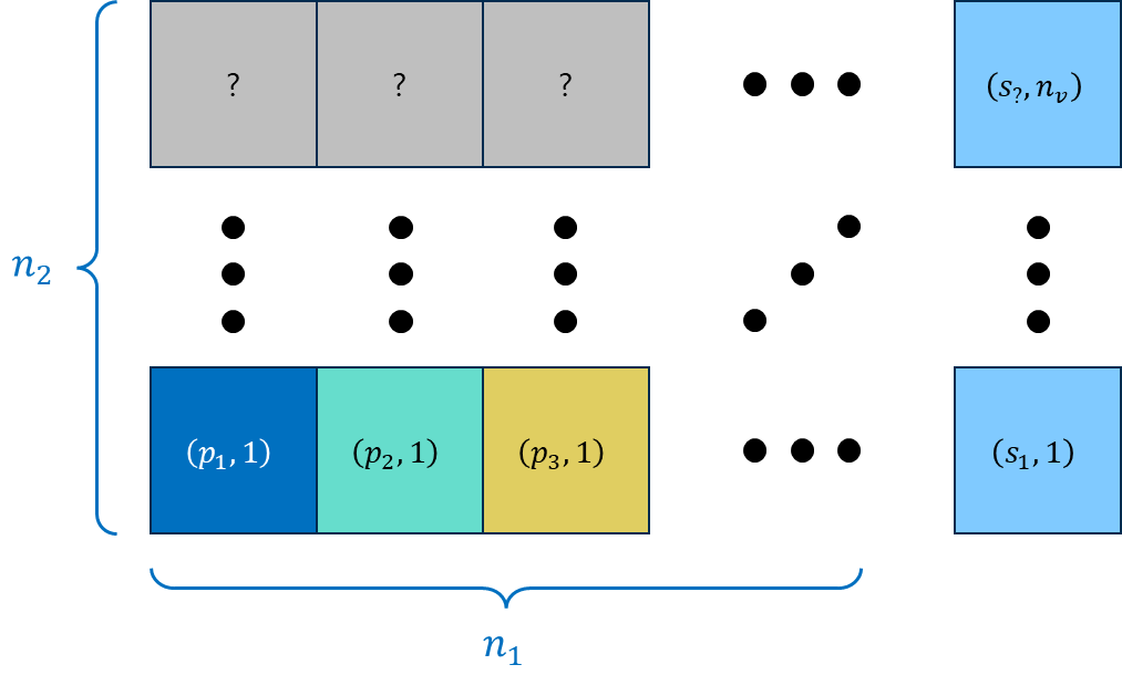
The system comprises individual cells with 2-entry tuples for labelling. The cells enclosed by the marking \(n_1\) and \(n_2\) are called primary cells, and the first entry in their labelling tuple contains ‘\(p\)’ (see Figure 1). Together, they are called Primary Grid (PG). On the other hand, the other cells are called secondary cells with the first entry in their labelling tuple containing ‘\(s\)’, and they are together called Secondary Grid (SG). Therefore, \(n_1\) is the number of stacks in PG, and \(n_2\) is the number of cells in each of these stacks. The complete labelling scenario in Figure 1 will be presented further in the theoretical development. All cells in the system form a larger grid referred to as the Entire Grid (EG). Combinatorial problems which can be modelled in this system will be referred to as Combinatorial Grid Sequencing (CGS) problems.
The most foundational notion introduced in the theory of CGS is a CGS space, which is given in the following definition.
Definition 3.1 (CGS Space). Let \(A_p, A_s\) be indexed sets such that
\[0 < |A_p|, |A_s| < \infty \;\land\; A_p \cap A_s = \varnothing \,, \tag{40}\] and these sets can be expressed as
\[A_p = \{p_1, \dotsc, p_{|A_p|}\} \,,\quad A_s = \{s_1, \dotsc, s_{|A_s|}\}, \tag{41}\] respectively. Some maps \(\omega_p: A_p \to \{1, \dotsc, |A_p|\}\) and \(\omega_s: A_s \to \{1, \dotsc, |A_s|\}\) satisfying
\[\forall k \in \{1, \dotsc, |A_p|\} \,,\; \omega_p(p_k) = k, \tag{42}\] and
\[\forall k \in \{1, \dotsc, |A_s|\} \,,\; \omega_s(s_k) = k, \tag{43}\] are called the natural orderings of \(A_p\) and \(A_s\) respectively. Let \(\mathbf{n} := (n_1, n_2) \in \mathbb{N}^2\) such that \(n_1, n_2 \geq 1\), and \(\mathbf{d} \in \mathbb{N}^\eta\), for some \(\eta \in \mathbb{N}\) with \(\eta \geq 1\). The tuple \((A_p, A_s, \mathbf{n}, \mathbf{d})\) is called a Combinatorial Grid Sequencing (CGS) space. The set \(A_p\) is referred to as the Primary Atomic Cells (PAC), and \(A_s\) is referred to as the Secondary Atomic Cells (SAC). The integer tuple \(\mathbf{n}\) is referred to as the shape of the CGS space, and \(\mathbf{d}\) as its dynamic parameters.
Intuitively, a CGS space provides the foundational setup upon which several other concepts for handling the CGS problem are built. It is worth noting that natural orderings on a CGS space are bijective, since PAC and SAC are naturally finite ordered sets. Now we present the first mapping of a CGS space, called the utilization map, as follows.
Definition 3.2 (Utilization Map). Let \((A_p, A_s, \mathbf{n}, \mathbf{d})\) be a CGS space. A map \(\rho: A_p \sqcup A_s \to \mathbb{N}\) defined by
\[\forall a_k \in A_p \sqcup A_s \,,\; \rho(a_k) := \begin{cases} \Big\lfloor \frac{n_1 n_2}{|A_p|} \Big\rfloor + 1 &: a_k \in A_p \land 0 < k \leq r_p, \\ \Big\lfloor \frac{n_1 n_2}{|A_p|} \Big\rfloor &: a_k \in A_p \land (r_p = 0 \lor k > r_p) ,\\ \Big\lfloor \frac{n_2}{|A_s|} \Big\rfloor + 1 &: a_k \in A_s \land 0 < k \leq r_s ,\\ \Big\lfloor \frac{n_2}{|A_s|} \Big\rfloor &: a_k \in A_s \land (r_s = 0 \lor k > r_s), \end{cases} \; \tag{44}\] where
\[r_p := n_1 n_2 – |A_p| \left\lfloor \frac{n_1 n_2}{|A_p|} \right\rfloor \,,\quad r_s := n_2 – |A_s| \left\lfloor \frac{n_2}{|A_s|} \right\rfloor \,, \tag{45}\] is called the utilization map of the CGS space.
Informally, the utilization map of a CGS space counts the total number of dynamic activities of the atomic cells within the CGS system. Now we proceed with the concept of EG, which corresponds to the tuple labelling in Figure 1.
Definition 3.3 (Entire Grid). Let \((A_p, A_s, \mathbf{n}, \mathbf{d})\) be a CGS space with \(\rho: A_p \sqcup A_s \to \mathbb{N}\) being its utilization map. The Entire Grid (EG) of the CGS space is a set
\[\mathcal{E} := \bigcup_{a \in A_p \sqcup A_s} \{a\} \times \{1, \dotsc, \rho(a)\} \,. \tag{46}\]
Each \((a, k) \in \mathcal{E}\) is referred to as a cell.
We have mentioned the notion of Primary Grid (PG) and Secondary Grid (SG) informally in the previous section. The formalization of these concepts is provided as follows.
Definition 3.4 (Primary and Secondary Grids). Let \((A_p, A_s, \mathbf{n}, \mathbf{d})\) be a CGS space with \(\rho: A_p \sqcup A_s \to \mathbb{N}\) being its utilization map and \(\mathcal{E}\) being its EG.
\[\mathcal{E}_p := \bigcup_{a \in A_p} \{a\} \times \{1, \dotsc, \rho(a)\}, \tag{47}\] is referred to as the Primary Grid (PG) of the CGS space.
\[\mathcal{E}_s := \bigcup_{a \in A_s} \{a\} \times \{1, \dotsc, \rho(a)\}, \tag{48}\] is referred to as the Secondary Grid (SG) of the CGS space.
A property regarding the relationship between the EG, PG, and SG of a CGS space can be deduced from Definition 3.3 and Definition 3.4. It is presented in the following theorem.
Theorem 3.5. Let \((A_p, A_s, \mathbf{n}, \mathbf{d})\) be a CGS space with \(\mathcal{E}, \mathcal{E}_p, \mathcal{E}_s\) being its EG, PG, and SG respectively, and \(\rho: A_p \sqcup A_s \to \mathbb{N}\) being its utilization map. The family \(\{\mathcal{E}_p, \mathcal{E}_s\}\) forms a partition of \(\mathcal{E}\).
Proof. By Definition 3.4 and \(A_p \cap A_s = \varnothing\) (see Definition 3.1), we obtain \[\begin{aligned} \mathcal{E}_p \cap \mathcal{E}_s &= \left( \bigcup_{a \in A_p} \{a\} \times \{1, \dotsc, \rho(a)\} \right) \cap \left( \bigcup_{a \in A_s} \{a\} \times \{1, \dotsc, \rho(a)\} \right) \\ &= \bigcup_{a \in A_p \cap A_s} \{a\} \times \{1, \dotsc, \rho(a)\} = \bigcup_{a \in \varnothing} \{a\} \times \{1, \dotsc, \rho(a)\} \\ &= \varnothing \,, \end{aligned}\] and by Definition 3.3 and Definition 3.4, we obtain \[\begin{aligned} \mathcal{E}_p \cup \mathcal{E}_s &= \left( \bigcup_{a \in A_p} \{a\} \times \{1, \dotsc, \rho(a)\} \right) \cup \left( \bigcup_{a \in A_s} \{a\} \times \{1, \dotsc, \rho(a)\} \right) \\ &= \bigcup_{a \in A_p \sqcup A_s} \{a\} \times \{1, \dotsc, \rho(a)\} \\ &= \mathcal{E} \,. \end{aligned}\]
Hence, \(\{\mathcal{E}_p, \mathcal{E}_s\}\) is a partition of \(\mathcal{E}\) [4]. ◻
Several fundamental properties of the PG and SG of a CGS space regarding their cardinalities are presented in the following two theorems.
Theorem 3.6. Let \((A_p, A_s, \mathbf{n}, \mathbf{d})\) be a CGS space with \(\rho: A_p \sqcup A_s \to \mathbb{N}\) being its utilization map and \(\mathcal{E}_p\) being its PG. The expression
\[|\mathcal{E}_p| = n_1 n_2, \tag{49}\] holds.
Proof. By Definition 3.4, we obtain
\[|\mathcal{E}_p| = \left| \bigcup_{a \in A_p} \{a\} \times \{1, \dotsc, \rho(a)\} \right| = \sum_{a \in A_p} \rho(a) \,. \tag{50}\]
Let
\[r_p := n_1 n_2 – |A_p| \left\lfloor \frac{n_1 n_2}{|A_p|} \right\rfloor, \tag{51}\] (see Definition 3.2). By Proposition 2.2, \(r_p\) is the remainder of a Euclidean division of \(n_1 n_2\) by \(|A_p|\) [8]. Hence, \(0 \leq r_p < |A_p|\). Let
\[q := \left\lfloor \frac{n_1 n_2}{|A_p|} \right\rfloor \,. \tag{52}\]
By Euclidean division [8], we have
\[n_1 n_2 = q |A_p| + r_p \,. \tag{53}\]
By Definition 3.2, we have
\[\forall a \in A_p \,,\; \rho(a) \in \{q + 1, q\} \,. \tag{54}\]
Specifically, there are \(r_p\) primary atomic cells in \(A_p\) whose \(\rho\) is equal to \(q + 1\), and there are \(|A_p| – r_p\) whose \(\rho\) is equal to \(q\). Consequently, we obtain
\[\sum_{a \in A_p} \rho(a) = (q + 1) r_p + q (|A_p| – r_p) = q |A_p| + r_p = n_1 n_2 \,. \tag{55}\]
Hence,
\[|\mathcal{E}_p| = \sum_{a \in A_p} \rho(a) = n_1 n_2, \tag{56}\] proves the theorem. ◻
Theorem 3.7. Let \((A_p, A_s, \mathbf{n}, \mathbf{d})\) be a CGS space with \(\rho: A_p \sqcup A_s \to \mathbb{N}\) being its utilization map and \(\mathcal{E}_s\) being its SG. The expression
\[|\mathcal{E}_s| = n_2, \tag{57}\] holds.
Proof. By Definition 3.4, we obtain
\[|\mathcal{E}_s| = \left| \bigcup_{a \in A_s} \{a\} \times \{1, \dotsc, \rho(a)\} \right| = \sum_{a \in A_s} \rho(a) \,. \tag{58}\]
Let
\[r_s := n_2 – |A_s| \left\lfloor \frac{n_2}{|A_s|} \right\rfloor, \tag{59}\] (see Definition 3.2). By Proposition 2.2, \(r_s\) is the remainder of a Euclidean division of \(n_2\) by \(|A_s|\) [8]. Hence, \(0 \leq r_s < |A_s|\). Let
\[q := \left\lfloor \frac{n_2}{|A_s|} \right\rfloor \,. \tag{60}\]
By Euclidean division [8], we have
\[n_2 = q |A_s| + r_s \,. \tag{61}\]
By Definition 3.2, we have
\[\forall a \in A_s \,,\; \rho(a) \in \{q + 1, q\} \,. \tag{62}\]
Specifically, there are \(r_s\) secondary atomic cells in \(A_s\) whose \(\rho\) is equal to \(q + 1\), and there are \(|A_s| – r_s\) whose \(\rho\) is equal to \(q\). Consequently, we obtain
\[\sum_{a \in A_s} \rho(a) = (q + 1) r_s + q (|A_s| – r_s) = q |A_s| + r_s = n_2 \,. \tag{63}\]
Hence,
\[|\mathcal{E}_s| = \sum_{a \in A_s} \rho(a) = n_2, \tag{64}\] proves the theorem. ◻
A direct implication of Theorem 3.5, Theorem 3.6, and Theorem 3.7 is a fundamental property of the EG of a CGS space, which is presented in the following corollary.
Corollary 3.8. Let \((A_p, A_s, \mathbf{n}, \mathbf{d})\) be a CGS space with \(\mathcal{E}\) being its EG. The expression
\[|\mathcal{E}| = (n_1 + 1) n_2, \tag{65}\] holds.
Proof. Recall that \(\mathcal{E}_p, \mathcal{E}_s \subset \mathcal{E}\) are the PG and SG of the CGS space. By Theorem 3.5, \(\{\mathcal{E}_p, \mathcal{E}_s\}\) is a partition of \(\mathcal{E}\), which implies that \(|\mathcal{E}| = |\mathcal{E}_p| + |\mathcal{E}_s|\) [4]. By Theorem 3.6 and Theorem 3.7, we obtain
\[|\mathcal{E}| = |\mathcal{E}_p| + |\mathcal{E}_s| = n_1 n_2 + n_2 = (n_1 + 1) n_2, \tag{66}\] which proves the corollary. ◻
Ordering becomes a crucial aspect of the EG of a CGS space. A particular type of ordering of EG, referred to as the lexicographic ordering (LO), is presented as follows.
Definition 3.9 (Lexicographic Ordering of EG). Let \((A_p, A_s, \mathbf{n}, \mathbf{d})\) be a CGS space with \(\mathcal{E}\) being its EG. The Lexicographic Ordering (LO) of \(\mathcal{E}\) is a map
\[\lambda: \mathcal{E} \to \{1, \dotsc, |\mathcal{E}|\}, \tag{67}\] defined by
\[\forall (a, k) \in \mathcal{E} \,,\; \lambda(a, k) := \begin{cases} \kappa_p(a, k) + \left\lfloor \frac{\kappa_p(a, k) – 1}{n_1} \right\rfloor &: (a, k) \in \mathcal{E}_p, \\ (n_1 + 1) \kappa_s(a, k) &: (a, k) \in \mathcal{E}_s, \end{cases} \; \tag{68}\] where \(\kappa_p: \mathcal{E}_p \to \mathbb{N}\) and \(\kappa_s: \mathcal{E}_s \to \mathbb{N}\) are defined by
\[\forall (a, k) \in \mathcal{E}_p \,,\; \kappa_p(a, k) := \omega_p(a) + (k – 1) |A_p|, \tag{69}\] and
\[\forall (a, k) \in \mathcal{E}_s \,,\; \kappa_s(a, k) := \omega_s(a) + (k – 1) |A_s|, \tag{70}\] respectively.
Intuitively, the LO of the EG of a CGS space enumerates the cells within the EG. It maps cell labelling of the form \((a, k)\) to an integer. A divisibility property related to the LO of the EG and the SG of a CGS space is presented in the following proposition.
Proposition 3.10. Let \((A_p, A_s, \mathbf{n}, \mathbf{d})\) be a CGS space with \(\mathcal{E}, \mathcal{E}_s\) being its EG and SG respectively, and \(\lambda: \mathcal{E} \to \{1, \dotsc, |\mathcal{E}|\}\) being the LO of the EG. By Definition 3.9, the divisibility property
\[\forall (a, k) \in \mathcal{E}[ (a, k) \in \mathcal{E}_s \implies n_1 + 1 \mid \lambda(a, k) ], \tag{71}\] holds.
While a similar divisibility property for the PG of a CGS space might not be as immediately obvious as the one in Proposition 3.10, it does hold, as presented in the following lemma.
Lemma 3.11. Let \((A_p, A_s, \mathbf{n}, \mathbf{d})\) be a CGS space with \(\mathcal{E}, \mathcal{E}_p\) being its EG and PG, and \(\lambda: \mathcal{E} \to \{1, \dotsc, |\mathcal{E}|\}\) being the LO of the EG. The expression
\[\forall (a, k) \in \mathcal{E}[ (a, k) \in \mathcal{E}_p \implies n_1 + 1 \nmid \lambda(a, k) ], \tag{72}\] holds.
Proof. Let \((a, k) \in \mathcal{E}_p\). By Definition 3.9, we have
\[\lambda(a, k) = \kappa_p(a, k) + \left\lfloor \frac{\kappa_p(a, k) – 1}{n_1} \right\rfloor \,. \tag{73}\]
By Euclidean division [8], there exists some \(q, r \in \mathbb{Z}\) such that
\[\kappa_p(a, k) – 1 = q n_1 + r, \tag{74}\] with \(0 \leq r < n_1\). And by Proposition 2.2,
\[q = \left\lfloor \frac{\kappa_p(a, k) – 1}{n_1} \right\rfloor \,, \tag{75}\] and we obtain
\[\kappa_p(a, k) = \left\lfloor \frac{\kappa_p(a, k) – 1}{n_1} \right\rfloor n_1 + r + 1 \,. \tag{76}\]
Combining the result above with the earlier one, we obtain \[\begin{aligned} \lambda(a, k) &= \left( \left\lfloor \frac{\kappa_p(a, k) – 1}{n_1} \right\rfloor n_1 + r + 1 \right) + \left\lfloor \frac{\kappa_p(a, k) – 1}{n_1} \right\rfloor \\ &= (n_1 + 1) \left\lfloor \frac{\kappa_p(a, k) – 1}{n_1} \right\rfloor + (r + 1) \,. \end{aligned}\]
Clearly, \(0 < r + 1 < n_1 + 1\). By Euclidean division, the expression above implies
\[n_1 + 1 \nmid \lambda(a, k) \,, \tag{77}\] which proves the lemma. ◻
Proposition 3.10 and Lemma 3.11 provide divisibility properties of SG and PG with respect to their LO values. The following theorem connects this entire relationship.
Theorem 3.12. Let \((A_p, A_s, \mathbf{n}, \mathbf{d})\) be a CGS space with \(\mathcal{E}, \mathcal{E}_p, \mathcal{E}_s\) being its EG, PG, and SG respectively, and \(\lambda: \mathcal{E} \to \{1, \dotsc, |\mathcal{E}|\}\) being the LO of the EG. The following conditions hold:
Proof. From Proposition 3.10, we have
\[\forall (a, k) \in \mathcal{E} [ (a, k) \in \mathcal{E}_s \implies n_1 + 1 \mid \lambda(a, k) ] \,, \tag{78}\] and from Lemma 3.11, we have
\[\forall (a, k) \in \mathcal{E} [ (a, k) \in \mathcal{E}_p \implies n_1 + 1 \nmid \lambda(a, k) ] \,. \tag{79}\]
(Proof for i) We will show that the converse of Expression (79) is true by contradiction. Let us assume that the converse is false. Then there exists some \((b, i) \in \mathcal{E}\) with \(n_1 + 1 \nmid \lambda(b, i)\) but \((b, i) \notin \mathcal{E}_p\). Since \(\{\mathcal{E}_p, \mathcal{E}_s\}\) is a partition of \(\mathcal{E}\) by Theorem 3.5, then \((b, i) \in \mathcal{E}_s\). However, it contradicts Expression (78). Hence,
\[\forall (a, k) \in \mathcal{E} [ n_1 + 1 \nmid \lambda(a, k) \implies (a, k) \in \mathcal{E}_p ] \,, \tag{80}\] which is the converse of Expression (79), must be true. Combined with Expression (79), it yields
\[\forall (a, k) \in \mathcal{E} [ (a, k) \in \mathcal{E}_p \iff n_1 + 1 \nmid \lambda(a, k) ], \tag{81}\] which proves condition (i). (Proof for ii) Likewise, we employ contradiction to prove the converse of Expression (78). Again, assume it is false, and there exists some \((c, j) \in \mathcal{E}\) with \(n_1 + 1 \mid \lambda(c, j)\) but \((c, j) \notin \mathcal{E}_s\). Again, since \(\{\mathcal{E}_p, \mathcal{E}_s\}\) is a partition of \(\mathcal{E}\), \((c, j) \in \mathcal{E}_p\) must hold. However, it is contradictory to Expression (79), concluding that
\[\forall (a, k) \in \mathcal{E} [ n_1 + 1 \mid \lambda(a, k) \implies (a, k) \in \mathcal{E}_s ], \tag{82}\] is necessarily true. Combined with Expression (78), it yields
\[\forall (a, k) \in \mathcal{E} [ (a, k) \in \mathcal{E}_s \iff n_1 + 1 \mid \lambda(a, k) ], \tag{83}\] which proves condition (ii). ◻
We now explore how to express a cell in the EG of a CGS space in terms of its LO image. We present a lemma containing three number-theoretic identities involving the floor function. One of the identities, which will be applied in the subsequent theorem, is instrumental for this purpose.
Lemma 3.13. Let \(a, b, c \in \mathbb{N}\) such that \(a, b, c \geq 1\) and
\[a = b + \left\lfloor \frac{b – 1}{c} \right\rfloor \,. \tag{84}\]
The following identities hold:
Proof. (Identity i) Let
\[q := \left\lfloor \frac{b – 1}{c} \right\rfloor \,. \tag{85}\]
Then we have
\[q \leq \frac{b – 1}{c} < q + 1 \,, \tag{86}\] which implies \(qc + 1 \leq b < (q + 1) c + 1\). Since \(b \in \mathbb{Z}\), then it becomes \(qc + 1 \leq b \leq (q + 1) c\). Note that \(a = b + q\). Hence,
\[q(c + 1) + 1 = (qc + 1) + q \leq b + q = a \leq ((q + 1) c + q) = q(c + 1) + c \,. \tag{87}\]
Dividing the inequality above by \(c + 1\), we obtain
\[q < q + \frac{1}{c + 1} = \frac{q(c + 1) + 1}{c + 1} \leq \frac{a}{c + 1} \leq \frac{q(c + 1) + c}{c + 1} = q + \frac{c}{c + 1} < q + 1, \tag{88}\] which implies
\[\left\lfloor \frac{a}{c + 1} \right\rfloor = q = \left\lfloor \frac{b – 1}{c} \right\rfloor \,. \tag{89}\]
(Identity ii) By substituting \(b + \left\lfloor \frac{b – 1}{c} \right\rfloor\) for \(a\) and applying identity i, we obtain
\[\left\lfloor \frac{b + \left\lfloor \frac{b – 1}{c} \right\rfloor}{c + 1} \right\rfloor = \left\lfloor \frac{b – 1}{c} \right\rfloor \,. \tag{90}\]
(Identity iii) Note that \(b = a – q\). By expanding \(q\) and applying identity i, we have
\[b = a – \left\lfloor \frac{b – 1}{c} \right\rfloor = a – \left\lfloor \frac{a}{c + 1} \right\rfloor \,. \tag{91}\]
Then by substituting the expression above for \(b\) into identity i, we obtain
\[\left\lfloor \frac{a}{c + 1} \right\rfloor = \left\lfloor \frac{b – 1}{c} \right\rfloor = \left\lfloor \frac{a – \left\lfloor \frac{a}{c + 1} \right\rfloor – 1}{c} \right\rfloor, \tag{92}\] which concludes the proof. ◻
Theorem 3.14. Let \((A_p, A_s, \mathbf{n}, \mathbf{d})\) be a CGS space with \(\mathcal{E}, \mathcal{E}_p, \mathcal{E}_s\) being its EG, PG, and SG respectively, and \(\lambda: \mathcal{E} \to \{1, \dotsc, |\mathcal{E}|\}\) being the LO of the EG. Let \((a, k) \in \mathcal{E}\) and \(m \in \{1, \dotsc, |\mathcal{E}|\}\) such that
\[\lambda(a, k) = m \,. \tag{93}\]
Then \(a\) and \(k\) can be expressed in terms of \(m\) by
\[k = \begin{cases} \bigg\lfloor \frac{m – \left\lfloor \frac{m}{n_1 + 1} \right\rfloor – 1}{|A_p|} \bigg\rfloor + 1 &: n_1 + 1 \nmid m, \\ \bigg\lfloor \frac{\frac{m}{n_1 + 1} – 1}{|A_s|} \bigg\rfloor + 1 &: n_1 + 1 \mid m, \end{cases} \tag{94}\] and
\[a = \begin{cases} \omega_p^{-1} \left( m – \left\lfloor \frac{m}{n_1 + 1} \right\rfloor – (k – 1) |A_p| \right) &: n_1 + 1 \nmid m, \\ \omega_s^{-1} \left( \frac{m}{n_1 + 1} – (k – 1) |A_s| \right) &: n_1 + 1 \mid m, \end{cases} \tag{95}\] respectively.
Proof. (First case). Suppose \(n_1 + 1 \nmid m\), which means \((a, k) \in \mathcal{E}_p\) by Theorem 3.12. By Definition 3.9 and identity i of Lemma 3.13, we obtain
\[\left\lfloor \frac{m}{n_1 + 1} \right\rfloor = \left\lfloor \frac{\kappa_p(a, k) – 1}{n_1} \right\rfloor \,, \tag{96}\] and again by Definition 3.9, we obtain \[\begin{aligned} m – \left\lfloor \frac{m}{n_1 + 1} \right\rfloor – 1 &= \kappa_p(a, k) + \left\lfloor \frac{\kappa_p(a, k) – 1}{n_1} \right\rfloor – \left\lfloor \frac{m}{n_1 + 1} \right\rfloor – 1 \\ &= \kappa_p(a, k) + \left\lfloor \frac{m}{n_1 + 1} \right\rfloor – \left\lfloor \frac{m}{n_1 + 1} \right\rfloor – 1 \\ &= \kappa_p(a, k) – 1 = \omega_p(a) + (k – 1)|A_p| – 1 \\ &= (k – 1)|A_p| + (\omega_p(a) – 1) \,. \end{aligned}\]
Note that \(0 \leq \omega_p(a) – 1 < |A_p|\). Hence, the expression above is a Euclidean division where the expression on the left side is the dividend, \(|A_p|\) is the divisor, \(k – 1\) is the quotient and \(\omega_p(a) – 1\) is the remainder [8]. By Proposition 2.2, we obtain
\[k = \left\lfloor \frac{m – \left\lfloor \frac{m}{n_1 + 1} \right\rfloor – 1}{|A_p|} \right\rfloor + 1 \,. \tag{97}\]
Recursively, we also obtain
\[a = \omega_p^{-1} \left( m – \left\lfloor \frac{m}{n_1 + 1} \right\rfloor – (k – 1) |A_p| \right), \tag{98}\] from the earlier expression.
(Second case). Suppose \(n_1 + 1 \mid m\), which means \((a, k) \in \mathcal{E}_s\) by Theorem 3.12. By Definition 3.9, we obtain
\[m = (n_1 + 1) \kappa_s(a, k) = (n_1 + 1) (\omega_s(a) + (k – 1)|A_s|) \,. \tag{99}\]
By rearranging the expression above and then subtracting \(1\) from both sides, we obtain
\[\frac{m}{n_1 + 1} – 1 = (k – 1) |A_s| + (\omega_s(a) – 1) \,. \tag{100}\]
Note that the left-hand side of the expression above is an integer since \(n_1 + 1 \mid m\), and \(0 \leq \omega_s(a) – 1 < |A_s|\). Hence, the expression above is a Euclidean division where the left-hand side is the dividend, \(|A_s|\) is the divisor, \(k – 1\) is the quotient and \(\omega_s(a) – 1\) is the remainder [8]. By Proposition 2.2, we obtain
\[k = \left\lfloor \frac{\frac{m}{n_1 + 1} – 1}{|A_s|} \right\rfloor + 1, \tag{101}\] and recursively, we obtain
\[a = \omega_s^{-1} \left( \frac{m}{n_1 + 1} – (k – 1) |A_s| \right), \tag{102}\] from the earlier expression. (All cases). From both cases, we obtain
\[k = \begin{cases} \bigg\lfloor \frac{m – \left\lfloor \frac{m}{n_1 + 1} \right\rfloor – 1}{|A_p|} \bigg\rfloor + 1 &: n_1 + 1 \nmid m, \\ \bigg\lfloor \frac{\frac{m}{n_1 + 1} – 1}{|A_s|} \bigg\rfloor + 1 &: n_1 + 1 \mid m, \end{cases} \tag{103}\] and
\[a = \begin{cases} \omega_p^{-1} \left( m – \left\lfloor \frac{m}{n_1 + 1} \right\rfloor – (k – 1) |A_p| \right), &: n_1 + 1 \nmid m, \\ \omega_s^{-1} \left( \frac{m}{n_1 + 1} – (k – 1) |A_s| \right) &: n_1 + 1 \mid m, \end{cases} \tag{104}\] which prove the theorem. ◻
Now we define another map based on Theorem 3.14, which is presented in the following definition.
Definition 3.15 (Anti-Lexicographic). Let \((A_p, A_s, \mathbf{n}, \mathbf{d})\) be a CGS space with \(\mathcal{E}, \mathcal{E}_p, \mathcal{E}_s\) being its EG, PG, and SG respectively, and \(\lambda: \mathcal{E} \to \{1, \dotsc, |\mathcal{E}|\}\) being the LO of the EG. A map \(\mu: \mathrm{im}\, \lambda \to \mathcal{E}\) defined by
\[\mu(m) = (a, k), \tag{105}\] with
\[k = \begin{cases} \bigg\lfloor \frac{m – \left\lfloor \frac{m}{n_1 + 1} \right\rfloor – 1}{|A_p|} \bigg\rfloor + 1 &: n_1 + 1 \nmid m, \\ \bigg\lfloor \frac{\frac{m}{n_1 + 1} – 1}{|A_s|} \bigg\rfloor + 1 &: n_1 + 1 \mid m, \end{cases} \tag{106}\] and
\[a = \begin{cases} \omega_p^{-1} \left( m – \left\lfloor \frac{m}{n_1 + 1} \right\rfloor – (k – 1) |A_p| \right) &: n_1 + 1 \nmid m, \\ \omega_s^{-1} \left( \frac{m}{n_1 + 1} – (k – 1) |A_s| \right) &: n_1 + 1 \mid m, \end{cases} \tag{107}\] for every \(m \in \mathrm{im}\, \lambda\), is called the Anti-Lexicographic (AL) map of the CGS space.
We need to first confirm that the AL map is well-defined, as provided in the following proposition.
Proposition 3.16. Let \((A_p, A_s, \mathbf{n}, \mathbf{d})\) be a CGS space with \(\mathcal{E}, \mathcal{E}_p, \mathcal{E}_s\) being its EG, PG, and SG respectively, \(\lambda: \mathcal{E} \to \{1, \dotsc, |\mathcal{E}|\}\) being the LO of the EG, and \(\mu: \mathrm{im}\, \lambda \to \mathcal{E}\) being its AL map. The property
\[\forall m, m’ \in \mathrm{im}\, \lambda [ m = m’ \implies \mu(m) = \mu(m’) ] \,, \tag{108}\] which states that \(\mu\) is a well-defined map, holds.
Proof. Let \(m, m’ \in \mathrm{im}\, \lambda\) such that \(m = m’\). Let \((a, k) = \mu(m)\) and \((a’, k’) = \mu(m’)\). Since \(m = m’\), by Theorem 3.14, we obtain \[\begin{aligned} k &= \begin{cases} \bigg\lfloor \frac{m – \left\lfloor \frac{m}{n_1 + 1} \right\rfloor – 1}{|A_p|} \bigg\rfloor + 1 &: n_1 + 1 \nmid m \\ \bigg\lfloor \frac{\frac{m}{n_1 + 1} – 1}{|A_s|} \bigg\rfloor + 1 &: n_1 + 1 \mid m \end{cases} \\ &= \begin{cases} \bigg\lfloor \frac{m’ – \left\lfloor \frac{m’}{n_1 + 1} \right\rfloor – 1}{|A_p|} \bigg\rfloor + 1 &: n_1 + 1 \nmid m’ \\ \bigg\lfloor \frac{\frac{m’}{n_1 + 1} – 1}{|A_s|} \bigg\rfloor + 1 &: n_1 + 1 \mid m’ \end{cases} \\ &= k’ \,. \end{aligned}\]
From this result and Theorem 3.14, we also obtain \[\begin{aligned} a &= \begin{cases} \omega_p^{-1} \left( m – \left\lfloor \frac{m}{n_1 + 1} \right\rfloor – (k – 1) |A_p| \right) &: n_1 + 1 \nmid m \\ \omega_s^{-1} \left( \frac{m}{n_1 + 1} – (k – 1) |A_s| \right) &: n_1 + 1 \mid m \end{cases} \\ &= \begin{cases} \omega_p^{-1} \left( m’ – \left\lfloor \frac{m’}{n_1 + 1} \right\rfloor – (k’ – 1) |A_p| \right) &: n_1 + 1 \nmid m’ \\ \omega_s^{-1} \left( \frac{m’}{n_1 + 1} – (k’ – 1) |A_s| \right) &: n_1 + 1 \mid m’ \end{cases} \\ &= a’ \,. \end{aligned}\]
Hence,
\[\mu(m) = (a, k) = (a’, k’) = \mu(m’)\] concludes that \(\mu\) is a well-defined map. ◻
Now we explore an important property of both the LO of the EG of a CGS space and its AL. It is provided in the following lemma.
Lemma 3.17. Let \((A_p, A_s, \mathbf{n}, \mathbf{d})\) be a CGS space with \(\mathcal{E}, \mathcal{E}_p, \mathcal{E}_s\) being its EG, PG, and SG respectively, and \(\lambda: \mathcal{E} \to \{1, \dotsc, |\mathcal{E}|\}\) being the LO of the EG. The AL map \(\mu: \mathrm{im}\,\lambda \to \mathcal{E}\) is a left-inverse of \(\lambda\), i.e., \(\mu \circ \lambda = \mathrm{id}_{\mathcal{E}}: \mathcal{E} \to \mathcal{E}\).
Proof. Let \((a, k) \in \mathcal{E}\). First, suppose \((a, k) \in \mathcal{E}_p\). Then
\[(\mu \circ \lambda)(a, k) = \mu( \lambda(a, k) ) = \mu\left( \kappa_p(a, k) + \left\lfloor \frac{\kappa_p(a, k) – 1}{n_1} \right\rfloor \right) =: (\tilde{a}, \tilde{k}) \,. \tag{109}\]
Note that \(\kappa_p(a, k) \geq 1\) by Definition 3.9. Then by identity ii of Lemma 3.13, we have
\[\left\lfloor \frac{\kappa_p(a, k) + \left\lfloor \frac{\kappa_p(a, k) – 1}{n_1} \right\rfloor}{n_1 + 1} \right\rfloor = \left\lfloor \frac{\kappa_p(a, k) – 1}{n_1} \right\rfloor \,. \tag{110}\]
By Definition 3.15 and Eq. (110) above, we obtain \[\begin{aligned} \tilde{k} &= \left\lfloor \frac{ \kappa_p(a, k) + \left\lfloor \frac{\kappa_p(a, k) – 1}{n_1} \right\rfloor – \left\lfloor \frac{\kappa_p(a, k) + \left\lfloor \frac{\kappa_p(a, k) – 1}{n_1} \right\rfloor}{n_1 + 1} \right\rfloor -1 }{|A_p|} \right\rfloor + 1 \\ &= \left\lfloor \frac{ \kappa_p(a, k) + \left\lfloor \frac{\kappa_p(a, k) – 1}{n_1} \right\rfloor – \left\lfloor \frac{\kappa_p(a, k) – 1}{n_1} \right\rfloor -1 }{|A_p|} \right\rfloor + 1 \\ &= \left\lfloor \frac{ \kappa_p(a, k) -1 }{|A_p|} \right\rfloor + 1 \\ &= \left\lfloor \frac{\omega_p(a) – 1}{|A_p|} + k – 1 \right\rfloor + 1 \,. \end{aligned}\]
Note that \(0 \leq \frac{\omega_p(a) – 1}{|A_p|} < 1\). Hence,
\[\tilde{k} = \left\lfloor \frac{\omega_p(a) – 1}{|A_p|} + k – 1 \right\rfloor + 1 = (k – 1) + 1 = k \,. \tag{111}\]
Again, from Definition 3.15 and Eq. (110), we obtain \[\begin{aligned} \tilde{a} &= \omega_p^{-1}\left( \kappa_p(a, k) + \left\lfloor \frac{\kappa_p(a, k) – 1}{n_1} \right\rfloor – \left\lfloor \frac{\kappa_p(a, k) + \left\lfloor \frac{\kappa_p(a, k) – 1}{n_1} \right\rfloor}{n_1 + 1} \right\rfloor – (k – 1)|A_p| \right) \\ &= \omega_p^{-1}\left( \kappa_p(a, k) + \left\lfloor \frac{\kappa_p(a, k) – 1}{n_1} \right\rfloor – \left\lfloor \frac{\kappa_p(a, k) – 1}{n_1} \right\rfloor – (k – 1)|A_p| \right) \\ &= \omega_p^{-1}( \omega_p(a) + (k – 1)|A_p| – (k – 1)|A_p| ) = \omega_p^{-1}(\omega_p(a)) \\ &= a \,. \end{aligned}\]
Now suppose \((a, k) \in \mathcal{E}_s\). Then
\[(\mu \circ \lambda)(a, k) = \mu( \lambda(a, k) ) = \mu( (n_1 + 1) \kappa_s(a, k) ) =: (\tilde{a}, \tilde{k}) \,. \tag{112}\]
By Definition 3.15, we obtain \[\begin{aligned} \tilde{k} &= \left\lfloor \frac{\frac{(n_1 + 1) \kappa_s(a, k)}{n_1 + 1} -1}{|A_s|} \right\rfloor + 1 = \left\lfloor \frac{\kappa_s(a, k) – 1}{|A_s|} \right\rfloor + 1 \\ &= \left\lfloor \frac{\omega_s(a) + (k – 1)|A_s| -1}{|A_s|} \right\rfloor + 1 \\ &= \left\lfloor \frac{\omega_s(a) -1}{|A_s|} + k – 1 \right\rfloor + 1 \,. \end{aligned}\]
Note that \(0 \leq \frac{\omega_s(a) – 1}{|A_s|} < 1\). Then the expression above becomes
\[\tilde{k} = \left\lfloor \frac{\omega_s(a) -1}{|A_s|} + k – 1 \right\rfloor + 1 = (k – 1) + 1 = k \,. \tag{113}\]
Again, by Definition 3.15, we obtain \[\begin{aligned} \tilde{a} &= \omega_s^{-1} \left( \frac{(n_1 + 1) \kappa_s(a, k)}{n_1 + 1} – (k – 1)|A_s| \right) = \omega_s^{-1}( \kappa_s(a, k) – (k – 1)|A_s| ) \\ &= \omega_s^{-1}( \omega_s(a) + (k – 1)|A_s| – (k – 1)|A_s| ) = \omega_s^{-1}( \omega_s(a) ) \\ &= a \,. \end{aligned}\]
Hence, for both cases, we have
\[(\mu \circ \lambda)(a, k) = (a, k) \,, \tag{114}\] which shows that \(\mu \circ \lambda = \mathrm{id}_{\mathcal{E}}: \mathcal{E} \to \mathcal{E}\) is an identity map, implying that \(\mu\) is a left-inverse of \(\lambda\). ◻
Lemma 3.17 implies a fundamental property of the LO of the EG of a CGS space, which is presented in the following theorem.
Theorem 3.18. Let \((A_p, A_s, \mathbf{n}, \mathbf{d})\) be a CGS space with \(\mathcal{E}, \mathcal{E}_p, \mathcal{E}_s\) being its EG, PG, and SG respectively, and \(\lambda: \mathcal{E} \to \{1, \dotsc, |\mathcal{E}|\}\) being the LO of the EG. The LO \(\lambda\) is bijective.
Proof. Let \(\mu: \mathrm{im}\, \lambda \to \mathcal{E}\) be the AL map. Let \(m, m’ \in \mathrm{im}\, \lambda\) such that \(m = m’\). Then there exist some \((a, k), (a’, k’) \in \mathcal{E}\) such that \(\lambda(a, k) = m\) and \(\lambda(a’, k’) = m’\). By Definition 3.15 and Lemma 3.17, we obtain \[\begin{aligned} (a, k) &= (\mu \circ \lambda)(a, k) = \mu(\lambda(a, k)) \\ &= \mu(m) \\ &= \mu(m’) \\ &= \mu(\lambda(a’, k’)) = (\mu \circ \lambda)(a’, k’) \\ &= (a’, k’), \end{aligned}\] which shows that \(\lambda\) is injective. Since \(\lambda\) is injective and \(|\mathcal{E}| = |\{1, \dotsc, |\mathcal{E}|\}| < \infty\), then by Proposition 2.1, \(\lambda\) is bijective. ◻
Theorem 3.18 guarantees that the inverse of the LO of the EG of a CGS space exists. Then the following theorem demonstrates the construction of the inverse formula.
Theorem 3.19. Let \((A_p, A_s, \mathbf{n}, \mathbf{d})\) be a CGS space with \(\mathcal{E}, \mathcal{E}_p, \mathcal{E}_s\) being its EG, PG, and SG respectively, and \(\lambda: \mathcal{E} \to \{1, \dotsc, |\mathcal{E}|\}\) being the LO of the EG. (i) \(\mathrm{im}\,\lambda = \{1, \dotsc, |\mathcal{E}|\}\), and (ii) the AL map \(\mu: \mathrm{im}\,\lambda \to \mathcal{E}\) is the inverse of the LO, i.e., \(\mu = \lambda^{-1}\).
Proof. (i) Since \(\lambda\) is bijective by Theorem 3.18, then \(\mathrm{im}\,\lambda = \{1, \dotsc, |\mathcal{E}|\}\). (ii) We have shown that \(\mu\) is a left-inverse of \(\lambda\) in Lemma 3.17. Now we show that it is also a right-inverse of \(\lambda\) to conclude that it is in fact the inverse. Let \(m \in \{1, \dotsc, |\mathcal{E}|\}\). Then we have
\[(\lambda \circ \mu)(m) = \lambda(\mu(m)) = \lambda(a, k), \tag{115}\] where \((a, k) \in \mathcal{E}\). Suppose \(n_1 + 1 \nmid m\). Then \(k\) and \(a\) are given in accordance with Definition 3.15 by
\[k = \left\lfloor \frac{m – \left\lfloor \frac{m}{n_1 + 1} \right\rfloor – 1 }{|A_p|} \right\rfloor + 1, \tag{116}\] and
\[a = \omega_p^{-1}\left( m – \left\lfloor \frac{m}{n_1 + 1} \right\rfloor – (k – 1)|A_p| \right) \,. \tag{117}\]
By Definition 3.9, we have \[\begin{aligned} \kappa_p(a, k) &= \omega_p(a) + (k – 1)|A_p| \\ &= \omega_p \left( \omega_p^{-1}\left( m – \left\lfloor \frac{m}{n_1 + 1} \right\rfloor – (k – 1)|A_p| \right) \right) + (k – 1)|A_p| \\ &= m – \left\lfloor \frac{m}{n_1 + 1} \right\rfloor – (k – 1)|A_p| + (k – 1)|A_p| \\ &= m – \left\lfloor \frac{m}{n_1 + 1} \right\rfloor \,. \end{aligned}\]
By identity iii of Lemma 3.13, the negative term of the expression above has an equivalent expression given by
\[\left\lfloor \frac{m}{n_1 + 1} \right\rfloor = \left\lfloor \frac{m – \left\lfloor \frac{m}{n_1 + 1} \right\rfloor – 1}{n_1} \right\rfloor \,. \tag{118}\]
Then from the expression of \(\kappa_p(a, k)\) and the equivalence above, we obtain \[\begin{aligned} \lambda(a, k) &= \kappa_p(a, k) + \left\lfloor \frac{\kappa_p(a, k) – 1}{n_1} \right\rfloor \\ &= m – \left\lfloor \frac{m}{n_1 + 1} \right\rfloor + \left\lfloor \frac{m – \left\lfloor \frac{m}{n_1 + 1} \right\rfloor – 1}{n_1} \right\rfloor \\ &= m – \left\lfloor \frac{m}{n_1 + 1} \right\rfloor + \left\lfloor \frac{m}{n_1 + 1} \right\rfloor \\ &= m, \end{aligned}\] which shows that \((\lambda \circ \mu)(m) = m\) when \(n_1 + 1 \nmid m\). Now suppose \(n_1 + 1 \mid m\). Then \(k\) and \(a\) are given in accordance with Definition 3.15 by
\[k = \left\lfloor \frac{\frac{m}{n_1 + 1} – 1}{|A_s|} \right\rfloor + 1, \tag{119}\] and
\[a = \omega_s^{-1}\left( \frac{m}{n_1 + 1} – (k – 1)|A_s| \right) \,. \tag{120}\]
By Definition 3.9, we have \[\begin{aligned} \kappa_s(a, k) &= \omega_s(a) + (k – 1)|A_s| \\ &= \omega_s\left( \omega_s^{-1}\left( \frac{m}{n_1 + 1} – (k – 1)|A_s| \right) \right) + (k – 1)|A_s| \\ &= \frac{m}{n_1 + 1} – (k – 1)|A_s| + (k – 1)|A_s| \\ &= \frac{m}{n_1 + 1} \,. \end{aligned}\]
Then we can expand the expression of \(\lambda(a, k)\) in accordance with Definition 3.9, and from the expression of \(\kappa_s(a, k)\) above, we obtain
\[\lambda(a, k) = (n_1 + 1) \kappa_s(a, k) = (n_1 + 1) \frac{m}{n_1 + 1} = m, \tag{121}\] which shows that \((\lambda \circ \mu)(m) = m\) when \(n_1 + 1 \mid m\). Hence, we have \((\lambda \circ \mu)(m) = m\) for any \(m \in \{1, \dotsc, |\mathcal{E}|\}\), showing that \(\mu\) is also a right-inverse of \(\lambda\), i.e., \(\lambda \circ \mu = \mathrm{id}_{\{1, \dotsc, |\mathcal{E}|\}}\). Hence, we conclude that \(\mu\) is the inverse of \(\lambda\), i.e., \(\mu = \lambda^{-1}\). ◻
In this section, we present a framework to model the dynamics of cells in the EG of a CGS space by incorporating max-plus algebra [3].
First, we introduce the notion of CGS State Space (CGS-SS) in the following definition.
Definition 3.20 (CGS State Space). Let \((A_p, A_s, \mathbf{n}, \mathbf{d})\) be a CGS space with \(\mathcal{E}\) being its EG. A CGS State Space (CGS-SS) is a max-plus semimodule \(\mathbb{Z}_{\max}^{|\mathcal{E}|}\). Each semimodule element in \(\mathbb{Z}_{\max}^{|\mathcal{E}|}\) describes a state of \(\mathcal{E}\).
Now we present the concept of CGS Dynamic Matrix (CGS-DM), which is a max-plus matrix describing the dynamic relationship of cells in EG.
Definition 3.21 (CGS Dynamic Matrix). Let \((A_p, A_s, \mathbf{n}, \mathbf{d})\) be a CGS space with \(\mathcal{E}\) being its EG and \(\mathbb{Z}_{\max}^{|\mathcal{E}|}\) being its CGS-SS. Let \(\lambda: \mathcal{E} \to \{1, \dotsc, |\mathcal{E}|\}\) be the LO of the EG. Suppose max-plus matrix \(R \in \mathbb{Z}_{\max}^{|\mathcal{E}| \times |\mathcal{E}|}\) and let \(r_{ij} \in \mathbb{Z}_{\max}\) represent the \(ij\)-th entry of \(R\), for any \(i, j \in \{1, \dotsc, |\mathcal{E}|\}\). Matrix \(R\) is called a CGS Dynamic Matrix (CGS-DM) if and only if the following axioms hold:
Intuitively, Axiom D1 specifies that the dynamic relationship of a cell in the EG with its preceding cell with respect to the LO cannot be \(\varepsilon\), except it is a cell whose LO is congruent to \(1 \pmod{n_1 + 1}\). Referring to the geometric illustration in Figure 1, cells whose LO is congruent to \(1 \pmod{n_1 + 1}\) are cells on the far left. Axiom D2 specifies that the dynamic relationship between a cell with the one below it cannot be \(\varepsilon\). Axiom D3 specifies that the dynamic relationship of a cell with an earlier cell whose atomic cells are the same and the utilization value is smaller by a margin exactly \(1\) cannot be \(\varepsilon\). Axiom D4 specifies that the dynamic relationship of a cell with itself and with a cell with a lower LO value is equal to \(\varepsilon\). And a CGS-DM is completely determined by the dynamic parameters of a CGS space as specified by Axiom D5. Now we explore a matrix property of a CGS-DM as presented in the following proposition.
Proposition 3.22. Let \((A_p, A_s, \mathbf{n}, \mathbf{d})\) be a CGS space with \(\mathcal{E}\) being its EG and \(\mathbb{Z}_{\max}^{|\mathcal{E}|}\) being its CGS-SS. A CGS-DM \(R \in \mathbb{Z}_{\max}^{|\mathcal{E}| \times |\mathcal{E}|}\) is a strict lower triangular max-plus matrix.
Proof. By Axiom D4, for each entry \(r_{ij} \in \mathbb{Z}_{\max}\) in \(R\), we have \(r_{ij} = \varepsilon\) whenever \(i \leq j\), and this is consistent with Axioms D1 and D2. Now we will show that it is also consistent with Axiom D3. Suppose \((a_i, k_i) = \mu(i)\) and \((a_j, k_j) = \mu(j)\). By Axiom D3, if \(i \leq j\) and \(a_i \neq a_j\) or \(k_i \neq k_j + 1\) then \(r_{ij} = \varepsilon\). Let
\[\varphi \;\overset{\mathrm{def}}{\equiv}\; (a_j, k_j) = \lambda^{-1}(j) \land (a_i, k_i) = \lambda^{-1}(i) \land a_i = a_j \land k_i = k_j + 1. \tag{122}\]
We will show that the condition \(i \leq j\) and \(\varphi\) cannot be attained. Assume it can, then we have \(a_i = a_j\) and \(k_i = k_j + 1\) but \(i \leq j\). Note that we have either exactly \(n_1 + 1 \mid i, j\) or \(n_1 + 1 \nmid i, j\), and no mixes of these conditions since \(a_i = a_j\). Note that here we have \(\lambda(a_i, k_i) = i\) and \(\lambda(a_j, k_j) = j\). By Definition 3.9, we obtain \[\begin{aligned} j – i &= \left( \omega_p(a_j) + (k_j – 1)|A_p| + \left\lfloor \frac{\omega_p(a_j) + (k_j – 1)|A_p| – 1 }{n_1} \right\rfloor \right) \\ &\quad\quad – \left( \omega_p(a_i) + (k_i – 1)|A_p| + \left\lfloor \frac{\omega_p(a_i) + (k_i – 1)|A_p| – 1 }{n_1} \right\rfloor \right) \\ &= (k_j – k_i)|A_p| + \left\lfloor \frac{\omega_p(a_j) + (k_j -1) |A_p|}{n_1} \right\rfloor – \left\lfloor \frac{\omega_p(a_i) + (k_i -1) |A_p|}{n_1} \right\rfloor \\ &= (k_j – (k_j + 1))|A_p| + \left\lfloor \frac{\omega_p(a_j) + (k_j – 1)|A_p| – 1 }{n_1} \right\rfloor – \left\lfloor \frac{\omega_p(a_j) + k_j|A_p| – 1 }{n_1} \right\rfloor \\ &= -|A_p| + \left\lfloor \frac{\omega_p(a_j) + (k_j – 1)|A_p| – 1 }{n_1} \right\rfloor – \left\lfloor \frac{\omega_p(a_j) + k_j|A_p| – 1 }{n_1} \right\rfloor \\ &< 0, \end{aligned}\] whenever \(n_1 + 1 \nmid i, j\), and \[\begin{aligned} j – i &= (n_1 + 1) (\omega_s(a_j) + (k_j – 1)|A_s|) – (n_1 + 1) (\omega_s(a_i) + (k_i – 1)|A_s|) \\ &= (n_1 + 1) (\omega_s(a_j) – \omega_s(a_i) + (k_j – k_i)|A_s|) \\ &= (n_1 + 1)(\omega_s(a_j) – \omega_s(a_j) + (k_j – (k_j – 1))|A_s|) \\ &= -(n_1 + 1)|A_s| \\ &< 0, \end{aligned}\] whenever \(n_1 + 1 \mid i, j\), showing that \(i > j\) in both conditions. This is contradictory to our assumption. Hence, \(\varphi\) is false whenever \(i \leq j\). It concludes that \(r_{ij} = \varepsilon\) whenever \(i \leq j\), showing that \(R\) is a strict lower triangular max-plus matrix. ◻
The notion of CGS-DM plays a pivotal role in the construction of a CGS State Closure Operator (CGS-SCO), which is presented as follows.
Definition 3.23 (CGS State Closure Operator). Let \((A_p, A_s, \mathbf{n}, \mathbf{d})\) be a CGS space with \(\mathcal{E}\) being its EG and \(\mathbb{Z}_{\max}^{|\mathcal{E}|}\) being its CGS-SS. Let \(R \in \mathbb{Z}_{\max}^{|\mathcal{E}| \times |\mathcal{E}|}\) be a CGS-DM. The CGS State Closure Operator (CGS-SCO) of \(R\) is a map \(T_{\mathrm{C}}: \mathbb{Z}_{\max}^{|\mathcal{E}|} \to \mathbb{Z}_{\max}^{|\mathcal{E}|}\) which is defined by
\[\forall \mathbf{u} \in \mathbb{Z}_{\max}^{|\mathcal{E}|} \,,\; T_{\mathrm{C}}(\mathbf{u}) := R^{\ast} \otimes \mathbf{u} \,. \tag{123}\]
Intuitively, a CGS-SCO maps the state of a CGS system to a terminal state of the system. A terminal state of a CGS system is a state when no more changes occur except for internal processes. Definition 3.23 has not guaranteed that such a state can be attained with the possible counter argument that the states may change indefinitely. However, it is indeed guaranteed in the following proposition.
Proposition 3.24. Let \((A_p, A_s, \mathbf{n}, \mathbf{d})\) be a CGS space with \(\mathcal{E}\) being its EG and \(\mathbb{Z}_{\max}^{|\mathcal{E}|}\) being its CGS-SS. Suppose \(T_{\mathrm{C}}: \mathbb{Z}_{\max}^{|\mathcal{E}|} \to \mathbb{Z}_{\max}^{|\mathcal{E}|}\) is the CGS-SCO of a CGS-DM \(R \in \mathbb{Z}_{\max}^{|\mathcal{E}| \times |\mathcal{E}|}\). The property
\[\forall \mathbf{u} \in \mathbb{Z}_{\max}^{|\mathcal{E}|} \,,\; T_{\mathrm{C}}(\mathbf{u}) = R^{\ast(|\mathcal{E}|)} \otimes \mathbf{u}, \tag{124}\] holds.
Proof. By Proposition 3.22, \(R\) is a strict lower triangular matrix. Let \(\mathbf{u} \in \mathbb{Z}_{\max}^{|\mathcal{E}|}\). By Corollary 2.6, Definition 3.23 and Definition 2.8, we obtain \[\begin{aligned} T_{\mathrm{C}}(\mathbf{u}) &= R^{\ast} \otimes \mathbf{u} = \left( \bigoplus_{k = 0}^\infty R^{\otimes(k)} \right) \otimes \mathbf{u} \\ &= \left( \left( \bigoplus_{i = 0}^{|\mathcal{E}| -1} R^{\otimes(i)} \right) \oplus \left( \bigoplus_{j = |\mathcal{E}|}^\infty R^{\otimes(j)} \right) \right) \otimes \mathbf{u} \\ &= \left( \left( \bigoplus_{i = 0}^{|\mathcal{E}| -1} R^{\otimes(i)} \right) \oplus \boldsymbol{\varepsilon} \right) \otimes \mathbf{u} = \left( \bigoplus_{i = 0}^{|\mathcal{E}| -1} R^{\otimes(i)} \right) \otimes \mathbf{u} \\ &= R^{\ast(|\mathcal{E}|)} \otimes \mathbf{u}, \end{aligned}\] which proves the proposition. ◻
Since the Kleene star in Proposition 3.24 is truncated, the result is a valid element in \(\mathbb{Z}_{\max}^{|\mathcal{E}|}\) as a state which is a terminal state. A specific type of terminal states is called CGS Preprocessed State (CGS-Pre-St), which is formally defined as follows.
Definition 3.25 (Preprocessed State). Let \((A_p, A_s, \mathbf{n}, \mathbf{d})\) be a CGS space with \(\mathcal{E}\) being its EG and \(\mathbb{Z}_{\max}^{|\mathcal{E}|}\) being its CGS-SS. Let \(T_{\mathrm{C}}: \mathbb{Z}_{\max}^{|\mathcal{E}|} \to \mathbb{Z}_{\max}^{|\mathcal{E}|}\) be a CGS-SCO. Let \(\mathbf{u}_0 \in \mathbb{Z}_{\max}^{|\mathcal{E}|}\) be a predefined initial state of the EG. The CGS Preprocessed State (CGS-Pre-St) of \(\mathbf{u}_0\) is some \(\mathbf{u} \in \mathbb{Z}_{\max}^{|\mathcal{E}|}\) such that
\[\mathbf{u} = T_{\mathrm{C}}(\mathbf{u}_0) \,. \tag{125}\]
Each cell in EG is designated to undergo some internal process. A state after completing an internal process will be referred to as a post-processed state. Such an internal process is handled by an operator called CGS Internal Process Operator (CGS-IPO) which is formally as follows.
Definition 3.26 (Internal Process). Let \((A_p, A_s, \mathbf{n}, \mathbf{d})\) be a CGS space with \(\mathcal{E}\) being its EG and \(\mathbb{Z}_{\max}^{|\mathcal{E}|}\) being its CGS-SS. A CGS Internal Process Operator (CGS-IPO) is a map
\[T_{\mathrm{IP}}: \mathbb{Z}_{\max}^{|\mathcal{E}|} \to \mathbb{Z}_{\max}^{|\mathcal{E}|}, \tag{126}\] defined by
\[\forall \mathbf{u} \in \mathbb{Z}_{\max}^{|\mathcal{E}|} \,,\; T_{\mathrm{IP}}(\mathbf{u}) := D \otimes \mathbf{u}, \tag{127}\] where \(D \in \mathbb{Z}_{\max}^{|\mathcal{E}| \times |\mathcal{E}|}\) is a diagonal max-plus matrix called a CGS Internal Process Matrix (CGS-IPM) such that there exists a map \(\mathbf{d} \mapsto D\).
The existence of the map from the dynamic parameters to the CGS-IPM in Definition 3.26 means that the CGS-IPM is necessarily created from the dynamic parameters. Now we present the formal definition of CGS Post Processed State (CGS-Post-St) as follows.
Definition 3.27 (Post-Processed State). Let \((A_p, A_s, \mathbf{n}, \mathbf{d})\) be a CGS space with \(\mathcal{E}\) being its EG and \(\mathbb{Z}_{\max}^{|\mathcal{E}|}\) being its CGS-SS. Let \(T_{\mathrm{C}}: \mathbb{Z}_{\max}^{|\mathcal{E}|} \to \mathbb{Z}_{\max}^{|\mathcal{E}|}\) be a CGS-SCO, \(\mathbf{u}_0 \in \mathbb{Z}_{\max}^{|\mathcal{E}|}\) be a predefined initial state of the EG, and \(T_{\mathrm{IP}}: \mathbb{Z}_{\max}^{|\mathcal{E}|} \to \mathbb{Z}_{\max}^{|\mathcal{E}|}\) be a CGS-IPO with respect to some CGS-IPM \(D \in \mathbb{Z}_{\max}^{|\mathcal{E}| \times |\mathcal{E}|}\). The CGS Post-Processed State (CGS-Post-St) is some \(\mathbf{v} \in \mathbb{Z}_{\max}^{|\mathcal{E}|}\) such that
\[\mathbf{v} = (T_{\mathrm{IP}} \circ T_{\mathrm{C}})(\mathbf{u}_0) \,. \tag{128}\]
Note that CGS-Pre-St and CGS-Post-St are both called terminal states. This term is based on the fact that these states undergoes CGS-SCO. The last two general CGS Max-Plus Dynamics concepts introduced in this section are called CGS Functional (CGS-F) and CGS Final Outcome (CGS-FO). These concepts are presented in the following two definitions respectively.
Definition 3.28 (CGS Functional). Let \((A_p, A_s, \mathbf{n}, \mathbf{d})\) be a CGS space with \(\mathcal{E}\) being its EG and \(\mathbb{Z}_{\max}^{|\mathcal{E}|}\) being its CGS-SS. Let \(T_{\mathrm{C}}: \mathbb{Z}_{\max}^{|\mathcal{E}|} \to \mathbb{Z}_{\max}^{|\mathcal{E}|}\) be a CGS-SCO, and \(T_{\mathrm{IP}}: \mathbb{Z}_{\max}^{|\mathcal{E}|} \to \mathbb{Z}_{\max}^{|\mathcal{E}|}\) be a CGS-IPO with respect to some CGS-IPM \(D \in \mathbb{Z}_{\max}^{|\mathcal{E}| \times |\mathcal{E}|}\). Suppose a map \(C: \mathbb{Z}_{\max}^{|\mathcal{E}|} \to \mathbb{Z}_{\max}\) defined by
\[\forall (u_1, \dotsc, u_{|\mathcal{E}|}) \in \mathbb{Z}_{\max}^{|\mathcal{E}|} \,,\; C(\mathbf{u}) = C(u_1, \dotsc, u_{|\mathcal{E}|}) := \bigoplus_{k = 1}^{|\mathcal{E}|} u_k \,, \tag{129}\] which is referred to as the collapsing functional. The CGS Functional (CGS-F) is a map \(\mathfrak{T}: \mathbb{Z}_{\max}^{|\mathcal{E}|} \to \mathbb{Z}_{\max}\) defined by \(\mathfrak{T} := C \circ T_{\mathrm{IP}} \circ T_{\mathrm{C}} \,.\)
Definition 3.29 (CGS Final Outcome). Let \((A_p, A_s, \mathbf{n}, \mathbf{d})\) be a CGS space with \(\mathcal{E}\) being its EG and \(\mathbb{Z}_{\max}^{|\mathcal{E}|}\) being its CGS-SS. Let \(\mathfrak{T}: \mathbb{Z}_{\max}^{|\mathcal{E}|} \to \mathbb{Z}_{\max}\) be a CGS-F. Let \(\mathbf{u}_0 \in \mathbb{Z}_{\max}^{|\mathcal{E}|}\) be a predefined initial state of the EG. The CGS Final Outcome (CGS-FO) of \(\mathbf{u}_0\) is some \(v \in \mathbb{Z}_{\max}\) such that \(v = \mathfrak{T}(\mathbf{u}_0) \,.\)
Intuitively, a CGS-FO of an initial state is the image of the initial state under the corresponding CGS-F.
The fundamental linearity properties of CGS operators presented in this section are provided in the following proposition.
Proposition 3.30. Let \((A_p, A_s, \mathbf{n}, \mathbf{d})\) be a CGS space with \(\mathcal{E}\) being its EG and \(\mathbb{Z}_{\max}^{|\mathcal{E}|}\) being its CGS-SS.
We now explore CGS Max-Plus Dynamics with a special condition that the CGS-IPM is a max-plus scalar matrix, i.e., a max-plus matrix whose diagonal entries are constant and other entries are \(\varepsilon\). A special property of CGS-F under this condition is presented in the following proposition.
Proposition 3.31. Let \((A_p, A_s, \mathbf{n}, \mathbf{d})\) be a CGS space with \(\mathcal{E}\) being its EG and \(\mathbb{Z}_{\max}^{|\mathcal{E}|}\) being its CGS-SS. Let \(\Delta \in \mathbb{Z}_{\max}\). Let \(D \in \mathbb{Z}_{\max}^{|\mathcal{E}| \times |\mathcal{E}|}\) be a CGS-IPM such that there exists a map \(\mathbf{d} \mapsto \Delta\) and \(D = \Delta \otimes I_{|\mathcal{E}|}\). Let \(T_{\mathrm{C}}: \mathbb{Z}_{\max}^{|\mathcal{E}|} \to \mathbb{Z}_{\max}^{|\mathcal{E}|}\) be a CGS-SCO, \(C: \mathbb{Z}_{\max}^{|\mathcal{E}|} \to \mathbb{Z}_{\max}\) be the collapsing functional, and \(\mathfrak{T}: \mathbb{Z}_{\max}^{|\mathcal{E}|} \to \mathbb{Z}_{\max}\) be the CGS-F. The property
\[\forall \mathbf{u} \in \mathbb{Z}_{\max}^{|\mathcal{E}|} \,,\; \mathfrak{T}(\mathbf{u}) = \Delta \otimes C(T_{\mathrm{C}}(\mathbf{u})), \tag{130}\] holds.
Proof. Let \(\mathbf{u} \in \mathbb{Z}_{\max}^{|\mathcal{E}|}\) and \(R \in \mathbb{Z}_{\max}^{|\mathcal{E}| \times |\mathcal{E}|}\) be the CGS-DM that realizes \(T_{\mathrm{C}}\), and \(T_{\mathrm{IP}}: \mathbb{Z}_{\max}^{|\mathcal{E}|} \to \mathbb{Z}_{\max}^{|\mathcal{E}|}\) be the CGS-IPO of the \(D\). By Definition 3.28, Definition 3.26 and Proposition 3.24 we obtain
\[\mathfrak{T}(\mathbf{u}) = C(T_{\mathrm{IP}}(T_{\mathrm{C}}(\mathbf{u}))) = C( \Delta \otimes I_{|\mathcal{E}|} \otimes R^{\ast(|\mathcal{E}|)} \otimes \mathbf{u} ) = C( \Delta \otimes R^{\ast(|\mathcal{E}|)} \otimes \mathbf{u} ) \,. \tag{131}\]
Let \(\mathbf{v} \in \mathbb{Z}_{\max}^{|\mathcal{E}|}\) be the CGS-Pre-St, i.e.,
\[\mathbf{v} = (v_1, \dotsc, v_{|\mathcal{E}|}) = T_{\mathrm{C}}(\mathbf{u}) = R^{\ast(|\mathcal{E}|)} \otimes \mathbf{u} \,. \tag{132}\]
Then the earlier expression becomes \[\begin{aligned} \mathfrak{T}(\mathbf{u}) &= C( \Delta \otimes R^{\ast(|\mathcal{E}|)} \otimes \mathbf{u} ) = C(\Delta \otimes \mathbf{v}) \\ &= \bigoplus_{k = 1}^{|\mathcal{E}|} \Delta \otimes v_k = \Delta \otimes \bigoplus_{k = 1}^{|\mathcal{E}|} v_k = \Delta \otimes C(\mathbf{v}) \\ &= \Delta \otimes C(T_{\mathrm{C}}(\mathbf{u})), \end{aligned}\] which proves the proposition. ◻
In real-world CGS problems, it is important to find a CGS space that optimizes a certain designated objective function. Therefore, we briefly explore further the family of all CGS spaces and derive some of its properties.
We denote the family of all CGS spaces by \(\mathcal{G}\). Then \(\mathbf{G} \in \mathcal{G}\) is a short notation of a CGS space in Definition 3.1. For convenience, we employ the following convention for expressing concepts and properties of CGS spaces:
An important property of some CGS spaces with the same shape is presented in the following proposition.
Proposition 3.32. Let \(\mathbf{G}, \mathbf{H} \in \mathcal{G}\) such that \(\mathbf{n}^{\mathbf{G}} = \mathbf{n}^{\mathbf{H}}\). By Corollary 3.8, we have \(|\mathcal{E}^{\mathbf{G}}| = |\mathcal{E}^{\mathbf{H}}| =: \nu\). Let \(R_{\mathbf{G}}, R_{\mathbf{H}} \in \mathbb{Z}_{\max}^{\nu \times \nu}\) be the corresponding CGS-DMs, and \(D_{\mathbf{G}}, D_{\mathbf{H}} \in \mathbb{Z}_{\max}^{\nu \times \nu}\) be the corresponding CGS-IPMs. If \(R_{\mathbf{G}} \leq R_{\mathbf{H}}\) and \(D_{\mathbf{G}} \leq D_{\mathbf{H}}\) hold entry-wise, then
\[\forall \mathbf{u} \in \mathbb{Z}_{\max}^{\nu} \,,\; \mathfrak{T}^{\mathbf{G}}(\mathbf{u}) \leq \mathfrak{T}^{\mathbf{H}}(\mathbf{u}), \tag{133}\] holds.
Proof. Suppose \(R_{\mathbf{G}} \leq R_{\mathbf{H}}\) and \(D_{\mathbf{G}} \leq D_{\mathbf{H}}\) hold entry-wise. Each entry \(x_{ij}\) in \(D_{\mathbf{G}} \otimes R_{\mathbf{G}}^{\ast (\nu)}\) can be expressed as
\[x_{ij} = \bigoplus_{k = 1}^\nu \Delta_{(\mathbf{G}) ik} \otimes r_{kj}^{(\mathbf{G})}, \tag{134}\] where \(r_{ij}^{(\mathbf{G})}\) and \(\Delta_{(\mathbf{G}) ij}\) represent each entry in \(R_{\mathbf{G}}^{\ast (\nu)}\) and \(D_{\mathbf{G}}\) respectively. Likewise, for each entry \(y_{ij}\) in \(D_{\mathbf{H}} \otimes R_{\mathbf{H}}^{\ast (\nu)}\),
\[y_{ij} = \bigoplus_{k = 1}^\nu \Delta_{(\mathbf{H}) ik} \otimes r_{kj}^{(\mathbf{H})}, \tag{135}\] where \(r_{ij}^{(\mathbf{H})}\) and \(\Delta_{(\mathbf{H}) ij}\) represent each entry in \(R_{\mathbf{H}}^{\ast (\nu)}\) and \(D_{\mathbf{H}}\) respectively. By the idempotence of \(\oplus\) on \(\mathbb{Z}_{\max}\), the monotonicity property of \(\otimes\), and Proposition 2.11, we obtain \[\begin{aligned} x_{ij} &= \bigoplus_{k = 1}^\nu \Delta_{(\mathbf{G}) ik} \otimes r_{kj}^{(\mathbf{G})} = \max_{k \in \{1, \dotsc, \nu\}} \Delta_{(\mathbf{G}) ik} + r_{kj}^{(\mathbf{G})} \\ &\leq \max_{k \in \{1, \dotsc, \nu\}} \Delta_{(\mathbf{H}) ik} + r_{kj}^{(\mathbf{H})} = \bigoplus_{k = 1}^\nu \Delta_{(\mathbf{H}) ik} \otimes r_{kj}^{(\mathbf{H})} \\ &= y_{ij} \,, \end{aligned}\] and hence, \(D_{\mathbf{G}} \otimes R_{\mathbf{G}}^{\ast (\nu)} \leq D_{\mathbf{H}} \otimes R_{\mathbf{H}}^{\ast (\nu)}\) holds entry-wise. Let \(\mathbf{u} \in \mathbb{Z}_{\max}^{\nu}\). Consequently,
\[\mathbf{v} := D_{\mathbf{G}} \otimes R_{\mathbf{G}}^{\ast (\nu)} \otimes \mathbf{u} \leq D_{\mathbf{H}} \otimes R_{\mathbf{H}}^{\ast (\nu)} \otimes \mathbf{u} =: \mathbf{w}, \tag{136}\] also holds entry-wise. By Definition 3.28, we obtain \[\begin{aligned} \mathfrak{T}^{\mathbf{G}}(\mathbf{u}) &= (C^{\mathbf{G}} \circ T_{IP}^{\mathbf{G}} \circ T_C^{\mathbf{G}})(\mathbf{u}) = C^{\mathbf{G}}(\mathbf{v}) = \bigoplus_{k = 1}^\nu v_k = \max_{k \in \{1, \dotsc, \nu\}}{v_k} \\ &\leq \max_{k \in \{1, \dotsc, \nu\}}{w_k} = \bigoplus_{k = 1}^\nu w_k = C^{\mathbf{H}}(\mathbf{w}) = (C^{\mathbf{H}} \circ T_{IP}^{\mathbf{H}} \circ T_C^{\mathbf{H}})(\mathbf{u}) \\ &= \mathfrak{T}^{\mathbf{H}}(\mathbf{u}) \,, \end{aligned}\] which proves the proposition. ◻
Proposition 3.32 allows us to make a direct comparison of the CGS-FOs of two CGS spaces with the same shape.
In this section, we demonstrate an implementation of the theory of CGS to optimize the concrete-casting process in the construction of a 3-storey rectangular building.
In our scenario, the horizontal area of the construction is divided into 5 zones that look like strips from the plan-view. The reason why the horizontal division is made such a way is that the on-site concrete casting needs to be executed sequentially from one zone to the next adjacent zone to ensure the structural integrity of the whole area. Considering that the horizontal sequence starts from the left to right, the zone at the far right, which is zone 5 in our case, will be set to have a special sequencing treatment. The other 4 zones will have the same width, while zone 5 may be different. This is a common engineering practice either to find a nice measure of width for the 4 zones and let the remaining width be occupied by zone 5, or in certain conditions, there are special structural elements like stairs that are commonly placed on the edge of the building within zone 5. On the other hand, the vertical division is naturally defined by the floor levels, reflecting the bottom-up, floor-by-floor sequence of the concrete-casting process.
With this zoning division, CGS spaces modelling this scenario have the same shape given by
\[\mathbf{n} = (n_1, n_2) = (4, 3), \tag{137}\] where \(n_1 = 4\) is the number of zones other than zone 5 and \(n_2 = 3\) is the number of floors. This also means that these CGS spaces also share the same EG, denoted by \(\mathcal{E}\), with
\[|\mathcal{E}| = (n_1 + 1) n_2 = (4 + 1) 3 = 15, \tag{138}\] by Corollary 3.8. Hence, the EG of every CGS space modelling this problem will have 15 cells where each cell is a zone at a certain floor. Consequently, these CGS spaces also share the same PG, denoted by \(\mathcal{E}_p\), and the same SG, denoted by \(\mathcal{E}_s\). By Theorem 3.6 and Theorem 3.7, we have \(|\mathcal{E}_p| = n_1 n_2 = 4 \cdot 3 = 12\) and \(|\mathcal{E}_s| = n_2 = 3\).
Each zone in this division will be equipped with a set of concrete-casting equipment including formwork and shoring, and also materials such as rebars configured in accordance with the zone. Engineers are using a limited number of sets of these equipment, especially formwork and shoring. The PAC of a CGS space will model the equipment sets operating in four zones, and the SAC will model the equipment sets operating in zone 5.
Some natural restrictions for feasible PACs and SACs are that the cardinality of a feasible PAC cannot exceed the cardinality of the PG, and the cardinality of a feasible SAC cannot exceed the cardinality of the SG. Using a PAC with the cardinality equal to that of PG and an SAC with the cardinality equal to that of SG mean that we use a distinct set of equipment for a distinct cell in EG. This specific setup is already intuitively inefficient and unfavourable since the number of the equipment sets will magnify the renting price. In addition, all equipment sets cannot be installed all at once due to construction limitations such as concrete hardening duration, etc [15], making some equipment sets inevitably idle. Therefore, \(|\mathcal{E}_p| = 12\) and \(|\mathcal{E}_s| = 3\) are the maximum cardinalities of feasible PACs and SACs, respectively.
The equipment and materials in the construction also require information related to preparation, installation, service and disassembling durations. This information is to be encoded in the dynamic parameters of the CGS spaces. In our scenario, we fix the preparation duration to be 1 day, the installation duration to be 3 days, the service duration to be 14 days, and the disassembling duration to be 1 day. The service duration is assumed to already include the concrete hardening time that is sufficient for bearing the construction loads [15]. This information is modelled by the dynamic parameters
\[\mathbf{d} = (d_1, d_2, d_3, d_4) := (1, 3, 14, 1) \,. \tag{139}\]
Note that we also employ the same dynamic parameters for all CGS spaces that model this problem. In a more complex problem, some entries in the dynamic parameters can be included as the parameters to be determined in the optimization, e.g., by varying the service durations since it is dependent on concrete hardening time. Concrete hardening time can be engineered to be faster to some degree by adding a specific chemical admixture, and this aspect affects the construction costs [15]. We opt to omit this complexity for the demonstration purposes.
Sets of equipment and materials, and preparation, installation, service and disassembling durations contribute directly to both costs and time of the construction. Additionally, costs depend on time.. Our objective in this problem will be finding the CGS spaces with the least construction duration.
The search space of our optimization will be a subfamily
\[\mathcal{G}_{(\mathbf{n}, \mathbf{d})} := \left\{ (A_p, A_s, \mathbf{n}, \mathbf{d}) \in \mathcal{G} \;\middle|\; |A_p| \leq n_1 n_2 \land |A_s| \leq n_2 \right\}, \tag{140}\] of all CGS spaces \(\mathcal{G}\). The first objective function is given in terms of CGS-F by a map \(\psi: \mathcal{G}_{(\mathbf{n}, \mathbf{d})} \to \mathbb{Z}_{\max}\) which is defined by
\[\forall \mathbf{G} \in \mathcal{G}_{(\mathbf{n}, \mathbf{d})} \,,\; \psi(\mathbf{G}) := \mathfrak{T}^{\mathbf{G}}(\mathbf{e}_1), \tag{141}\] where \(\mathbf{e}_1 := (0, \varepsilon, \dotsc, \varepsilon) \in \mathbb{Z}_{\max}^{|\mathcal{E}|}\) is the predefined initial state for all CGS spaces in \(\mathcal{G}_{(\mathbf{n}, \mathbf{d})}\). The semimodule element \(\mathbf{e}_1\) is chosen because the work has not started on day zero, and the initial state is zero. With the definition of \(\psi\) in Eq. (141), the final outcome of a CGS space represents the total duration.
Our optimization problem will be a multistep optimization, which is formally presented as follows:
\[\forall \mathbf{G} \in \mathcal{G}’ \,,\; \psi(\mathbf{G}) = \min_{\mathbf{H} \in \mathcal{G}_{(\mathbf{n}, \mathbf{d})}} \psi(\mathbf{H}) \,. \tag{142}\]
\[\forall \mathbf{G} \in \mathcal{G}” \,,\; |A_p^{\mathbf{G}}| + |A_s^{\mathbf{G}}| = \min_{\mathbf{H} \in \mathcal{G}’} |A_p^{\mathbf{H}}| + |A_s^{\mathbf{H}}| \,. \tag{143}\]
\[\tilde{\mathbf{G}} = \underset{\mathbf{H} \in \mathcal{G}”}{\arg\min} \; |A_s^{\mathbf{H}}| \,. \tag{144}\]
In step O1, we search CGS spaces that minimize the CGS-FO. It ensures that our optimized solution has the least construction duration. Then in step O2 we search CGS spaces among these spaces which minimize the sum of the cardinalities of PAC and SAC. This is an attempt to get a solution with the least number of equipment sets, hence a less total construction cost. And then in step O3 we further search the CGS space among these spaces which minimizes the cardinality of SAC. We use an assumption that renting less equipment sets for zone 5 will further optimize the total construction cost.
The CGS-DM of a CGS space in this scenario describes the sequencing of the concrete-casting work and the dynamic relationship between cells in the EG. The CGS-DM also contains construction restrictions such as the work at the current cell cannot be executed before some activities at the cell on the left, bottom and the one that uses the same equipment set have been finished. Formally, we present the constructive definition of the CGS-DM of each \(\mathbf{G} \in \mathcal{G}_{(\mathbf{n}, \mathbf{d})}\) in the following procedure:
\[r_{ij} = \begin{cases} d_1 \otimes 1 &: i = j + 1 \;\;\land\;\; i \not\equiv 1 \pmod{n_1 + 1}, \\ \varepsilon &: i \neq j + 1 \;\;\lor\;\; i \equiv 1 \pmod{n_1 + 1} . \end{cases} \, \tag{145}\]
Matrix \(R_1^{\mathbf{G}}\) ensures that the cell exactly on the right of the current cell cannot start working until one day after the preparation work is finished in the current cell, except for the cell on the far left which has no precedence in the same floor level.
\[r_{ij} = \begin{cases} \bigotimes_{\alpha = 1}^4 d_\alpha &: i = j + \ell (n_1 + 1), \\ \varepsilon &: i \neq j + \ell (n_1 + 1). \end{cases} \, \tag{146}\]
Matrix \(R_2^{\mathbf{G}}\) ensures that the cell exactly above the current cell cannot start working until all activities in the current cell are finished, except for cells in the lowest floor level. This requirement is a structural engineering necessity, since formwork, shoring and other construction equipment cannot be installed on top of an area whose concrete structure has not sufficiently reached a capacity to bear construction loads.
\[r_{ij} = \begin{cases} \bigotimes_{\alpha = 1}^4 d_\alpha &: \varphi, \\ \varepsilon &: \neg \varphi, \end{cases} \tag{147}\] holds, where \(\varphi\) is a logical statement given by
\[\varphi \;\overset{\mathrm{def}}{\equiv}\; (a_j, k_j) = \mu(j) \land (a_i, k_i) = \mu(i) \land a_i = a_j \land k_i = k_j + 1 \,. \tag{148}\]
Matrix \(R_3^{\mathbf{G}}\) ensures that the current cell cannot start working if it uses the same equipment set which is still being used in a different cell. Therefore, the current cell must wait until this different cell completes its activities.
\[R^{\mathbf{G}} := \bigoplus_{\alpha = 1}^3 R_\alpha^{\mathbf{G}} \,. \tag{149}\]
The following proposition guarantees that the procedures above provide a valid construction for the CGS-DM of \(\mathbf{G}\).
Proposition 4.1. Matrix \(R^{\mathbf{G}}\) is a valid CGS-DM.
Proof. Let \(\mathcal{E}\) be the EG and \(\lambda: \mathcal{E} \to \{1, \dotsc, |\mathcal{E}|\}\) be the LO of \(\mathbf{G}\). Let \[\begin{aligned} L_1 &:= \{(i, j) \in \mathrm{im}\,\lambda^2 \mid i = j + 1 \;\land\; i \not\equiv 1 \pmod{n_1 + 1} \} \,, \\ L_2 &:= \{(i, j) \in \mathrm{im}\,\lambda^2 \mid \exists \ell \in \{1, \dotsc, n_2 -1\} [ i = j + \ell(n_1 + 1)] \} \,, \\ L_3 &:= \{(i, j) \in \mathrm{im}\,\lambda^2 \mid \varphi \} \,. \end{aligned}\]
Note that the entry labels of the non-\(\varepsilon\) entries in \(R^{\mathbf{G}}\) are in \(L_1 \cup L_2 \cup L_3\). And note that
\[\forall \alpha, \beta \in \{1, \dotsc, 3\} \,,\; L_\alpha \cap L_\beta = \varnothing \,. \tag{150}\]
By Eq. (139), we have \(d_1 = 1\). Then by step 1 in the procedure above, for each entry \(r_{ij}\) in \(R_1^{\mathbf{G}}\), we have \(r_{ij} = d_1 \otimes 1 = 1 \otimes 1 = 2 > \varepsilon\) whenever \(i = j + 1\) and \(i \not\equiv 1 \pmod{n_1 + 1}\), and \(r_{ij} = \varepsilon\) otherwise. With this condition and by Expression (150) as well as procedure 4, each entry \(r_{ij}\) in \(R^{\mathbf{G}}\) satisfies
\[i = j + 1 \;\land\; i \not\equiv 1 \pmod{n_1 + 1} \implies r_{ij} \neq \varepsilon \,, \tag{151}\] and consequently satisfies Axiom D1.
Let \(r_{ij}\) be an entry in \(R_2^{\mathbf{G}}\). If \(i = j + (n_1 + 1)\) or \(i = j + 2(n_1 + 1)\), Eq. (139) and step 2 of the procedure above implies
\[r_{ij} = \bigotimes_{\alpha = 1}^4 d_\alpha = d_1 \otimes d_2 \otimes d_3 \otimes d_4 = 1 \otimes 3 \otimes 14 \otimes 1 = 19 > \varepsilon \,, \tag{152}\] and otherwise, \(r_{ij} = \varepsilon\). With this condition and by Expression (150) as well as procedure 4, each entry \(r_{ij}\) in \(R^{\mathbf{G}}\) satisfies
\[\forall \ell \in \{1, 2\}[ i = j + \ell(n_1 + 1) \implies r_{ij} \neq \varepsilon ] \,, \tag{153}\] and consequently satisfies Axiom D2.
Let \(r_{ij}\) be an entry in \(R_3^{\mathbf{G}}\). If the logical statement \(\varphi\) in Eq. (148) is true, Eq. (139) and step 3 in the procedure above imply
\[r_{ij} = \bigotimes_{\alpha = 1}^4 d_\alpha = d_1 \otimes d_2 \otimes d_3 \otimes d_4 = 1 \otimes 3 \otimes 14 \otimes 1 = 19 > \varepsilon \,, \tag{154}\] and otherwise, \(r_{ij} = \varepsilon\). With this condition and by Expression (150) as well as procedure 4, each entry \(r_{ij}\) in \(R^{\mathbf{G}}\) satisfies
\[\varphi \implies r_{ij} \neq \varepsilon \,, \tag{155}\] and consequently satisfies Axiom D3.
By all procedures and Expression (150), and based on the argument in the proof of Proposition 3.22, each entry \(r_{ij}\) in \(R^{\mathbf{G}}\) satisfies
\[i \leq j \implies r_{ij} = \varepsilon \,, \tag{156}\] and consequently satisfies Axiom D4.
By the procedures above, for each \(\alpha \in \{1, 2, 3\}\), there is a map \(\mathbf{d} \mapsto R_\alpha^{\mathbf{G}}\) in procedure \(\alpha\). The mapping tuple of these maps forms an individual map \(\mathbf{d} \mapsto (R_1^{\mathbf{G}}, R_2^{\mathbf{G}}, R_3^{\mathbf{G}})\). Then by procedure 4, there is a map \((R_1^{\mathbf{G}}, R_2^{\mathbf{G}}, R_3^{\mathbf{G}}) \mapsto R^{\mathbf{G}}\) defined by the \(\oplus\). Hence, there is a map \(\mathbf{d} \mapsto R^{\mathbf{G}}\) from all the procedures defined by the composition chain
\[\mathbf{d} \mapsto (R_1^{\mathbf{G}}, R_2^{\mathbf{G}}, R_3^{\mathbf{G}}) \mapsto R^{\mathbf{G}}, \tag{157}\] which satisfies Axiom D5. ◻
Proposition 4.1 and Eq. (149) show that \(R^{\mathbf{G}}\) is a valid CGS-DM by Definition 3.21. An algorithmic implementation for computing our constructed CGS-DM is provided as follows (Algorithm 1).
Algorithm 1. Implementation of CGS-DM
In our problem, the total work duration of activities in each cell is set to be identical. And the CGS-IPM of \(\mathbf{G}\) is given by a scalar matrix
\[D := \Delta \otimes I_{15} := \left( \bigotimes_{\alpha = 1}^4 d_\alpha \right) \otimes I_{15} = (1 \otimes 3 \otimes 14 \otimes 1) \otimes I_{15} = 19 \otimes I_{15} \,. \tag{158}\]
For this demonstration, we opt to implement an exhaustive method, that is, by testing every single CGS space in \(\mathcal{G}_{(\mathbf{n}, \mathbf{d})}\). This method is feasible if we have a small search space, otherwise, it is highly inefficient.
To justify the use of the exhaustive method, we now check the size of the search space. Note that the variations in \(\mathcal{G}_{(\mathbf{n}, \mathbf{d})}\) are only on the PACs and SACs, while the shape of CGS spaces and the dynamic parameters are fixed to \(\mathbf{n} = (4, 3)\) and \(\mathbf{d} = (1, 3, 14, 1)\) respectively. As mentioned earlier, the maximum number of PAC variations is \(|\mathcal{E}_p| = n_1 n_2 = 12\), while the maximum number of SAC variations is \(|\mathcal{E}_s| = n_2 = 3\). Hence, the size of the search space is given by
\[|\mathcal{G}_{(\mathbf{n}, \mathbf{d})}| = |\mathcal{E}_p| \cdot |\mathcal{E}_s| \cdot |\{\mathbf{n}\}| \cdot |\{\mathbf{d}\}| = 12 \cdot 3 \cdot 1 \cdot 1 = 36 \,. \tag{159}\]
This number is quite small, and it justifies that the use of exhaustive method is fairly feasible.
Now we present the algorithm for computing \(\psi: \mathcal{G}_{(\mathbf{n}, \mathbf{d})} \to \mathbb{Z}_{\max}\), given as Algorithm 2. This algorithm is created based on the formal definition of CGS-F (Definition 3.28) and CGS-FO (Definition 3.29).
Algorithm 2. Implementation of the Function \(\psi\)
And the optimization algorithm implementing the exhaustive method, by following steps O1, O2 and O3, is presented as Algorithm 3.
Algorithm 3. Optimization
We implement the algorithms using Python in a JupyterLab notebook [9]. The notebook is available at [11]. Our computation shows that the optimized solution is given by the CGS space \((A_p, A_s, \mathbf{n}, \mathbf{d})\) with \(|A_p| = 4\) and \(|A_s| = 1\), and a final outcome of 65. Consequently, the total duration of the concrete-casting work is determined to be 65 days. This number is the least, since other CGS spaces have 82, 118 and 230 as their final outcomes.
To evaluate the practical feasibility of the theory, Algorithm 3 was benchmarked using the aforementioned Python implementation. For the search space \(\mathcal{G}_{(\mathbf{n}, \mathbf{d})}\) defined in Eq. (140), the empirical execution time was 1.10 seconds. This test was conducted on a Ryzen 7 8700F CPU with 16GB Dual-Channel DDR5 RAM. Notably, the computation is strictly CPU-bound, requiring no GPU acceleration.
While the search space is limited to 36 candidates (Eq. (159)), manual evaluation in current engineering practice remains a significant bottleneck. Standard construction industry procedures typically involve manual spreadsheet entries or basic scheduling software, which requires hours to resolve the complex dependency checks for a single sequence, and even days to evaluate the entire set of possible candidates. This type of problem was also echoed in [1]. Our implementation reduces the evaluation of the entire search space to seconds, effectively replacing a heuristic, error-prone manual process with a rigorous, automated optimization.
The relationship between the theory of CGS and graph theory lies in the CGS-DM, which can also be interpreted as an adjacency matrix in terms of graph theory [3]. In this case, cells in an EG of a CGS space can be interpreted as vertices of a graph and the dynamic relationship between cells in the EG can be interpreted as edges and weights. With the result from our practical problem given in Section 4.4, our optimized CGS space is given by
\[(A_p, A_s, \mathbf{n}, \mathbf{d}) = (\{p_1, p_2, p_3, p_4\}, \{s_1\}, (4, 3), (1, 3, 14, 1)) \,, \tag{160}\] and the corresponding CGS-DM is given by a \(15 \times 15\) max-plus matrix below:
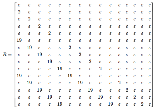
The graph representation of CGS-DM \(R \in \mathbb{Z}_{\max}^{15 \times 15}\) above is given by \(G = (V, E, w)\) where
\[V = \{v_1, \dotsc, v_{15}\}, \tag{161}\] is the set of all vertices in the graph,
\[E = E_1 \sqcup E_2, \tag{162}\] is the set of all edges in the graph where \[\begin{aligned} E_1 &= \{(v_i, v_{i + 1}) \mid i \in \{1, \dotsc, 14\} \setminus \{5, 10\} \} \,, \\ E_2 &= \{(v_i, v_{i + 5}) \mid i \in \{1, \dotsc, 10\} \} \,, \end{aligned}\] and \(w: E \to \mathbb{Z}_{\max}\) is the weight function defined via \(R\) by
\[\forall i, j \in \{1, \dotsc, 15\} \,,\; w(v_j, v_i) := r_{ij}, \tag{163}\] where \(r_{ij}\) is an entry in \(R\). The graph \(G\) is a digraph [3]. And the lower triangularity of \(R\), as guaranteed by Proposition 3.22, shows that \(G\) is a directed acyclic graph (DAG) [3].
The existence of graph \(G\) as the translation of the CGS space \((A_p, A_s, \mathbf{n}, \mathbf{d})\) demonstrates an equivalence between the two theories for this specific civil engineering construction problem. To be precise, it is the EG \(\mathcal{E}\) of \((A_p, A_s, \mathbf{n}, \mathbf{d})\) and CGS-DM \(R\) that are directly equivalent to graph \(G\). However, graph \(G\) is agnostic to the underlying configurations of the problem including the number of equipment sets in use. It makes the optimization objectives in steps O2 and O3 not possible with this setup. Therefore, the theory of CGS provides more automation compared to graph theory for such a grid-sequencing problem.
This paper has introduced the axiomatic framework of Combinatorial Grid Sequencing (CGS), starting from the foundational concept of a CGS space. We developed its associated orderings and constructed sets, namely the Entire Grid (EG), Primary Grid (PG), and Secondary Grid (SG), together with the fundamental ordering on EG called the Lexicographic Ordering (LO). We have also shown that LO admits an explicitly constructed inverse, the Anti-Lexicographic (AL) map. Notably, the derivation of this inverse led to the independent discovery of three number-theoretic identities involving the floor function in Lemma 3.13, which are essential for the AL map’s closed-form expression and the proof that the AL map is the inverse of LO.
We have further presented the framework for describing the dynamics within a CGS system called CGS Max-Plus Dynamics (CGS-MPD) by incorporating max-plus algebra. We have also explored a special condition of CGS-IPM when it is a scalar matrix, and we have presented its consequences in Proposition 3.31 which forms the basis for the architecture of Algorithm 2. Algorithm 2 is instrumental for the application presented in Section 4. Furthermore, we have explored the family of all CGS spaces and deduced a monotonicity property of a certain subfamily of CGS spaces with the same shape. This monotonicity property allows a direct comparison between two CGS spaces within the subfamily.
We have also demonstrated a computational application of the theory of CGS to optimize the total time of the concrete-casting in a three-storey building construction problem with two additional constraints related to the number of equipment sets used for the construction as presented in Section 4. The implementation of the theory of CGS successfully delivers the construction-sequencing configuration that minimizes the total time of the concrete-casting work under the assumed circumstances. The empirical computational runtime, which was 1.10 seconds given the hardware specification mentioned in Section 4.4, provides a glimpse into how an implementation of CGS can help speed up such engineering tasks significantly, compared to the industry standard practice which usually takes hours to days for the same tasks.
We have also explored a brief parallel between graph theory and the theory of CGS, demonstrating an equivalence in the specific case provided in Section 4.5. While graph-based models focus on connectivity, they remain structurally agnostic to the foundational configurations in our problem, specifically regarding the types of equipment sets. CGS spaces, by contrast, natively encode these parameters within the foundational configuration, allowing for a more representative and automated optimization process.
This framework has the potential to provide a foundation for optimization in identifying a CGS space that optimizes the CGS-FO or other objective functions associated with CGS spaces. It enables engineers to develop algorithms for automated CGS simulations, ultimately supporting systematic computational optimization.
For future work, we aim to implement the theory of CGS for a more complex civil engineering construction optimization problem. We also aspire to further generalize the current theory of CGS, such as allowing the SAC to be an empty set in future work.
The computational simulations supporting the findings of this study are available in a JupyterLab notebook hosted on GitHub at https://github.com/rizalpurnawan23/Combinatorial-Grid-Sequencing/blob/main/cgs_application_01/cgs-impl.ipynb
and are also archived on Zenodo (DOI: 10.5281/zenodo.21248849).
This work was supported by the Department of Civil and Environmental Engineering, Engineering Faculty, at Universitas Gajah Mada through the Research Grant No. 1610402/UN1.FTK/SK/HK/2025. We are grateful for the department’s continued commitment to advancing scholarly inquiry and for the resources that made this project possible.
| AL | Anti-Lexicographic |
| BIM | Building Information Modelling |
| CGS | Combinatorial Grid Sequencing |
| CGS-DM | CGS Dynamic Matrix |
| CGS-F | CGS Functional |
| CGS-FO | CGS Final Outcome |
| CGS-IPM | CGS Internal Process Matrix |
| CGS-IPO | CGS Internal Process Operator |
| CGS-MPD | CGS Max-Plus Dynamics |
| CGS-Pre-St | CGS Preprocessed State |
| CGS-Post-St | CGS Post Processed State |
| CGS-SS | CGS State Space |
| EG | Entire Grid |
| LO | Lexicographic Ordering |
| PAC | Primary Atomic Cells |
| PG | Primary Grid |
| SAC | Secondary Atomic Cells |
| SG | Secondary Grid |
| \(A_p\) | A set denoting a PAC |
| \(A_s\) | A set denoting an SAC |
| \(C\) | A map denoting the collapsing functional, but also context-dependent |
| \(\mathbf{d}\) | A tuple of \(\eta\) entries of positive integers, denoting the dynamic parameters of a CGS space, for some positive integer \(\eta\) |
| \(d_1\) | An integer which is the first entry of \(\mathbf{d}\) |
| \(d_2\) | An integer which is the second entry of \(\mathbf{d}\) |
| \(d_3\) | An integer which is the third entry of \(\mathbf{d}\) |
| \(d_4\) | An integer which is the fourth entry of \(\mathbf{d}\) |
| \(d_\eta\) | An integer which is \(\eta\)-th entry of \(\mathbf{d}\) |
| \(D\) | A max-plus matrix denoting a CGS-IPM/also context-dependent |
| \(\mathbf{n}\) | A tuple of two entries of positive integers, denoting the shape of a CGS space |
| \(n_1\) | A positive integer which is the first entry of \(\mathbf{n}\) |
| \(n_2\) | A positive integer which is the second entry of \(\mathbf{n}\) |
| \(R\) | A max-plus matrix denoting a CGS-DM/also context-dependent |
| \(T_{\mathrm{C}}\) | A map denoting a CGS-SCO |
| \(T_{\mathrm{IP}}\) | A map denoting a CGS-IPO |
| \(\mathcal{E}\) | A set denoting the EG of a CGS space |
| \(\mathcal{E}_p\) | A set denoting the PG of a CGS space |
| \(\mathcal{E}_s\) | A set denoting the SG of a CGS space |
| \(\mathfrak{T}\) | A map denoting a CGS-F |
| \(\lambda\) | A map denoting the LO of a CGS space |
| \(\omega_p\) | A map denoting the natural ordering of \(A_p\) |
| \(\omega_s\) | A map denoting the natural ordering of \(A_s\) |
| \(\mu\) | A map denoting the AL of a CGS space |
| \(\rho\) | A map called the utilization map of a CGS space |
Standard mathematical notation is used for all other symbols unless otherwise specified.