
The strategic management of the enterprise can combine the development trend of the market, the competitive advantages of the enterprise in the industry and the development needs of the enterprise to clarify the development direction and formulate the relevant strategic planning [26, 13]. In addition, the strategic management of the enterprise can also eectively supervise and control the overall operation of the enterprise, improve the implementation ability and efficiency of the enterprise, and improve the comprehensive strength of the enterprise as well as its position in the industry. Therefore, the strategic management of the enterprise has an important role and far-reaching influence on the development of the enterprise [3, 25, 16, 10].
The strategic management of the enterprise can carry out a complete planning for the operation of the enterprise, help the management personnel of the enterprise to make the correct decision which is helpful to the development of the enterprise, the strategic management has formulated the stage development planning for the enterprise in the process of development, and clarified the development goal of the enterprise in the current stage, which effectively promotes the development of the enterprise and improves the economic efficiency of the enterprise [29, 12, 23].
There must be different risks in the operation process of the enterprise, whether it can do a good job of risk prevention, identification, and effectively reduce the risk to the enterprise brought about by the loss of economic benefits and loss of social benefits, is a key factor in determining whether the enterprise can be long-term prosperity and development [4, 21]. Strategic management can accurately predict and prevent risks that have not occurred. For the risks that have already occurred in the market, the strategic management of the enterprise can minimize the losses brought by the risks to the enterprise. Therefore, strategic management is one of the most common risk management measures in enterprises nowadays [24, 22]. However, due to the ever-changing and unpredictable market environment, only the use of strategic management means of risk management can not guarantee the long-term development of the enterprise, in addition, the enterprise should also when the development of specific risk prevention system to ensure the sustainable development of the enterprise [28, 1].
The holistic nature of strategic management is the overall time, strategic management of the development of the enterprise can be a global long-term control, the development of the enterprise to play a guiding role. The strategic management of the enterprise can examine the market environment from a scientific point of view, help the enterprise to formulate the “future” development plan, to ensure that the development plan for the future long-term development of the enterprise has applicability [30, 27]. The existence of healthy competition in the market is an important factor to promote the development of more enterprises, from the perspective of strategic management, enterprises can stand on the industry’s high point of the entire market review, through the analysis of the market value chain, the enterprise’s own value chain and competitors’ value chain to fully understand the market situation, improve the inadequacies of the enterprise’s operations in a timely manner, and improve the enterprise’s competitiveness in the industry [2, 5].
In recent years with the rapid development of China’s market economy, China has appeared in the problems of high resource consumption, serious environmental pollution, and lack of independent innovation ability [14]. In the fierce market competition how can we completely get rid of the high dependence on low cost and highlight the competition, this is the problem that many enterprises need to be solved urgently at present [18]. All along, the rational allocation and use of resources is to ensure the survival and development of enterprises is a key link, only with sufficient resources to ensure the efficient operation of modern enterprises, but this inadvertently increases the cost of enterprises, if the enterprise’s resources are seriously insufficient to ensure that the future development of enterprises, the normal operation of the future development of the enterprise will bring about a serious impact and crisis [8, 7]. At the current stage of social and economic development, it is not difficult to see that, relative to the needs of customers, the resources have been embodied in the relative scarcity, therefore, this requires that modern enterprises must be on the scarce, limited resources for rational allocation, with the least amount of resource consumption to produce and provide the most suitable for the market demand for products and services, and to take this as an opportunity to win the best economic benefits [11, 17, 20].
The article firstly analyzes and models the proportion of resource allocation at the time of enterprise strategic management, and establishes a multi-parameter multi-objective resource allocation model. Secondly, it describes the principle of the Gray Wolf optimization algorithm and designs the improvement process of the Gray Wolf optimization algorithm, including the ways to improve the initial population range, convergence factor and dynamic weights. Expanding the diversity of the initial population and improving the convergence factor to a nonlinear factor enhance the ability of the algorithm to expand the search range and promote the balance between local optimization and global search. Changing the gray wolf leadership decision weights improves the accuracy of the algorithm in a dynamic weighting manner. Then the improved Gray Wolf algorithm is compared with the Gray Wolf algorithm and its variants, and five new swarm intelligence optimization algorithms in comparison experiments using 12 benchmark test functions and the CEC2017 test function set, respectively. Finally, simulation experiments are carried out as an example of resource allocation when the enterprise is intelligent, and the improved algorithm is used to solve the model, which further verifies the feasibility of the algorithm of this paper in solving practical problems.
Let the resources that an enterprise can invest in order to be intelligent be \(R=\{ H,F,T,D\}\), \(H\) denotes human resources, \(F\) denotes capital, \(T\) denotes time, and \(D\) denotes equipment [9]. And in order to achieve the expected benefits of the enterprise through intelligent transformation under the condition of limited resources, it is necessary to rationally allocate these several resources.
The core of the intelligent benefits of the enterprise is competitiveness and profitability. Then, the intelligent benefit can be expressed as \(E=(P,G)\), \(P\) for competitiveness and \(G\) for profitability. \[\label{GrindEQ__1_} \left\{\begin{array}{l} {\varphi _{1} :{\rm Exist\; }P>0}, \\ {P=(r_{1} \times w_{1,1} +r_{2} \times w_{1,2} +\cdots +r_{n} \times w_{1,n} )-Q_{1} }, \\ {n=|R|}, \\ {0<w_{1,n} \le 1}, \end{array}\right.\tag{1}\] where \(r_{n}\) represents the amount of resources available for type \(n\), \(w_{1,n}\) represents the proportion of resources allocated to type \(n\), and \(Q\) is the uncertainty of losses due to other constraints. \[\label{GrindEQ__2_} \left\{\begin{array}{l} {\varphi _{2} :{\rm Exist\; }G>0}, \\ {G=(r_{1} \times w_{2,1} +r_{2} \times w_{2,2} +\cdots +r_{n} \times w_{2,n} )-Q_{2} }, \\ {n=|R|}, \\ {0<w_{2,n} \le 1}. \end{array}\right.\tag{2}\]
Then, intelligent benefit \(E\) is further portrayed in mathematical language as: \[\label{GrindEQ__3_} \left\{\begin{array}{l} {RW^{T} -Q=(r_{ij} )_{m\times n} \times (w_{1} ,w_{2} ,\cdots ,w_{n} )^{T} -Q=E}, \\ {E=(e_{1} ,e_{2} ,\cdots ,e_{m} )^{T} }. \end{array}\right.\tag{3}\]
In the formula, \(W\) is the allocation ratio matrix of each resource, and \(R\) is the matrix of the number of various types of resources. After setting the expected intelligent benefits of the enterprise \(E\), it is necessary to find the allocation ratio of various resources \(W\), so as to achieve the expected benefits. However, the reality is that the number of various resources can be invested is limited, it is difficult to find a perfect coefficient matrix \(W\), so that the value of \(R\times W\) and \(E\) is infinitely close to the difference of 0. The optimization objective is: to find a resource allocation ratio matrix \(W=(w_{1} ,w_{2} ,\cdots ,w_{n} )^{T} ,(r_{ij} )_{m\times n} \times W_{n\times 1} -Q_{m\times 1} =Y_{m\times 1} ,Y=(y_{1} ,y_{2} ,\cdots ,y_{m} )^{{\rm T}}\), so that the minimum \(\left(\sum\limits_{i}= 1^{m} (y_{i} -e_{i} )^{2} /m\right)^{1/2}\). The optimization objective is defined as: \[\label{GrindEQ__4_} \left\{\begin{array}{l} {\varphi _{3} :\min \left(\sum\limits_{i=1}^{m}(y_{i} -e_{i} )^{2} /m\right)^{1/2} }, \\ {0<w_{j} \le 1}, \\ {0<r_{i} \le R_{e} }, \\ {\sum\limits_{i=1}^{n}w_{j} \times r_{i} \le Sum(R_{i} )}. \end{array}\right.\tag{4}\]
From (4), it can be seen that the closer its value is to 0, the better it is and the closer it is to the maximum benefit of intelligence [15].
The core of the idea of the gray wolf optimization algorithm originates from the action mode taken by the gray wolf population when they hunt collectively in nature.GWO is a new kind of group intelligence optimization algorithm, which completes the optimization process of the objective by simulating the hunting mode of the gray wolf group and obtains the corresponding optimization results. Now we will call the four ranks by \(\alpha ,\beta ,\delta ,\omega\) wolf, and the ranks are from high to low. And with reference to the process of hunting implementation, the algorithm is divided into three steps, which are: dividing the social class, tracking the prey, and hunting. When the hunting goal is accomplished, the value of the optimal solution is obtained as the location of \(\alpha\) wolves. From the perspective of mathematical theory, the details of the GWO algorithm in modeling these three stages are as follows.
Social hierarchy stratification.
In each hunting process, the gray wolf population, which has a strict social hierarchy in nature, will first complete the social hierarchy and elect \(\alpha ,\beta ,\delta ,\omega\) wolves, and the individual gray wolves will perform their own duties according to their own hierarchy.
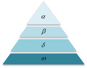
The gray wolf algorithm hierarchy is shown in Figure 1, the whole wolf population is divided into \(\alpha ,\beta ,\delta ,\omega\) wolves of four ranks, and the ranks are arranged in order from high to low [6]. And \(\alpha ,\beta ,\delta\) wolves ranked the top three in the whole population in terms of adaptability, which is at the top of the population, these gray wolves not only have strong adaptive ability, but also have the leadership responsibility for the lower level wolves.
Tracking prey.
After the hierarchical stratification is completed, the GWO initializes the position of \(\alpha ,\beta ,\delta ,\omega\) wolves for analysis, while defining their position relative to the prey, and then tracks the prey, and the position of \(\alpha ,\beta ,\delta ,\omega\) wolves is continuously updated during the optimization process, as well.
Eq. (5) represents the distance between individual gray wolves, and Eq. (6) represents how the gray wolf positions are updated. \[\label{GrindEQ__5_} X^{t+1} =X_{p}^{t} -AD,\tag{5}\] \[\label{GrindEQ__6_} D=|CX_{p}^{t} -X^{t} |,\tag{6}\] where \(t\) is the number of iterations of the action, \(X_{p}^{T}\) is the position of the prey at the \(t\)th iteration and \(X^{t}\) is the position of the individual gray wolf at the \(t\)th iteration. \[\label{GrindEQ__7_} A=2ar_{1} -a.\tag{7}\]
The random variable \(A\) is the main parameter of the gray wolf algorithm, which controls the size of the gray wolf population. When \(|A|>1\), gray wolves should try to spread out and search for prey in each region. When \(|A|\le 1\), the gray wolves will concentrate their search for prey in one or more areas. \[\label{GrindEQ__8_} C=2r_{2} ,\tag{8}\] \[\label{GrindEQ__9_} a=2-2\left(\frac{t}{\max } \right),\tag{9}\] where \(C\) denotes a perturbation to the prey and \(r_{1} ,\) \(r_{2}\) are arbitrary values that are in the interval [0, 1]. The convergence factor \(a\) is the master of parameter \(A\), which is linearly decreasing in the interval [0, 2] and \(t\) denotes the current number of iterations and max denotes the maximum value of the number of iterations.
Hunting.
During the final stage of hunting, the leading wolves discover the location of the prey. The \(\alpha\) wolves formulate the hunting strategy and guide the entire gray wolf population toward the prey [19]. The \(\alpha\), \(\beta\), and \(\delta\) wolves are assumed to be the closest to the prey, and thus, the direction and step size of all other wolves are updated based on their positions.
Let the position of a wolf at iteration \(t+1\) be denoted by \(X^{t+1}\). The vector \(A\) represents an adaptive coefficient, and the movement directions and step lengths of the remaining wolves relative to the positions of the \(\alpha\), \(\beta\), and \(\delta\) wolves are defined as follows:
\[\label{GrindEQ__10_} \begin{cases} X_{1} = X_{\alpha} – A_{1} D_{\alpha}, \\ X_{2} = X_{\beta} – A_{2} D_{\beta}, \\ X_{3} = X_{\delta} – A_{3} D_{\delta}, \end{cases}\tag{10}\]
where \(X_{\alpha}\), \(X_{\beta}\), and \(X_{\delta}\) represent the positions of the \(\alpha\), \(\beta\), and \(\delta\) wolves, respectively. The coefficients \(C_1\), \(C_2\), and \(C_3\) are random vectors. Let \(X^t\) denote the current position of a wolf in the population. The distance vectors \(D_{\alpha}\), \(D_{\beta}\), and \(D_{\delta}\) between the wolves and the leading wolves at iteration \(t\) are given by:
\[\label{GrindEQ__11_} \begin{cases} D_{\alpha} = |C_{1} X_{\alpha} – X^t|, \\ D_{\beta} = |C_{2} X_{\beta} – X^t|, \\ D_{\delta} = |C_{3} X_{\delta} – X^t|. \end{cases}\tag{11}\]
Finally, the new position of the wolf at iteration \(t+1\) is computed as the average of the three influence directions:
\[\label{GrindEQ__12_} X^{t+1} = \frac{X_{1} + X_{2} + X_{3}}{3}.\tag{12}\]
The solution of GWO has to be first divided into \(\alpha ,\beta ,\delta\) wolf, by which three layers of wolves are just hunting the position of the target, updating the position of the other gray wolves on the basis of when the position of the \(\alpha ,\beta ,\delta\) wolves, and finally on the siege target. The gray wolf algorithm wolf hunting schematic is shown in Figure 2.

The solution of GWO has to be first divided into \(\alpha ,\beta ,\delta\) wolf, by which three layers of wolves are just hunting the position of the target, updating the position of the other gray wolves on the basis of when the position of \(\alpha ,\beta ,\delta\) wolves, and finally on the siege target. The flowchart of the gray wolf optimization algorithm is shown in Figure 3:

Optimizing initial population strategy.
The inverse learning strategy can increase the diversity of the population so as to avoid the phenomenon of early maturity, and its main idea is to solve a feasible solution corresponding to the inverse solution, and evaluate both of them, and choose the best as the next generation of individuals. Here, the gray wolf population size is assumed to be \(\; N\), the search space dimension is \(\; d\), and \(x_{i} =(x_{i1} ,x_{i2} ,…,x_{id} )\) is the spatial location of the \(i\)th gray wolf individual.
Reverse solution: Assuming that a feasible solution of the current population is \(X=(x_{1} ,x_{2} ,\\\ldots ,x_{i} ,\ldots ,x_{N} )(x_{i} \in [a_{i} ,b_{i} ])\), its reverse solution is \(\bar{X}=(\overline{x_{1} },\overline{x_{2} },\ldots ,\overline{x_{i} },\ldots ,\overline{x_{N} })\), where \(\bar{x}_{i} =\lambda (a_{i} +b_{i} )-x_{i}\), \(\lambda\) are the coefficients of the uniform distribution in the interval [0, 1]. Elite reverse learning is the method of increasing the diversity of the initial population by creating reverse solutions and choosing one of the current and reverse solutions as the optimal solution for the new generation.
Elite inverse solution: Assume that the extreme point of an individual in the population is an elite individual, i.e., \(X_{i,j}^{e} =(X_{i,3}^{e} ,X_{i,2}^{e} ,…,X_{i,d}^{e} )\), where \(i=(1,2,\ldots ,N),j=(1,2,\ldots ,d)\), defines its inverse solution \(\bar{X}_{i,j}^{e} =(\overline{X_{i,1}^{e} },\overline{X_{i,2}^{e} },\ldots ,\overline{X_{i,d}^{e} })\) as: \[\label{GrindEQ__13_} \overline{X_{i,j}^{e} }=K\cdot (\chi _{j} +\delta _{j} )-X_{i,j}^{e} ,\tag{13}\] where \(K\) is the dynamic coefficient on the interval (0, 1), \(X_{i} ,j^{e} \in \left[\chi _{j} ,\delta _{j} \right],\chi _{j} =\min (X_{i,j} )\), \(\chi _{j}\) and \(\delta _{j}\) are the dynamic boundary. The dynamic boundary can overcome the shortcomings of difficult to preserve the search experience, so that the inverse solution of the elite strategy can be searched in a narrow space, and is not easy to fall into the local optimum. If \(\overline{x_{i,j}^{e} }\) crosses the boundary and becomes a non-feasible solution, it can be reset using a random generation method as follows: \[\label{GrindEQ__14_} \overline{X_{i,j}^{e} }=rand(\chi _{j} ,\delta _{j} ).\tag{14}\]
Improvement based on nonlinear convergence factor.
In this paper, an exponential \(a\)-decision algorithm is selected for the convergence process, and the function is expressed as: \[\label{GrindEQ__15_} a=2-2(2^{\frac{t}{\max } } -1)=4-2^{\frac{t}{\max } +1} ,\tag{15}\] where \(t\) represents the number of iterations and \(\max\) represents the maximum number of iterations.
Improvement based on dynamic weights.
The \(\omega\) wolves need to summarize the relative position information of the \(\alpha ,\beta ,\delta\) wolves to decide their moving direction and distance, and the three leader wolves all have equal influence on the \(\omega\) wolves, and set the same weights for all position information. In the algorithm, \(\alpha ,\beta ,\delta\) wolves must be the top three solutions in terms of fitness function values. In the algorithm solution, making \(\alpha ,\beta ,\delta\) wolves guide the other wolves in the pack with exactly the same power is obviously inconsistent with reality, which will firstly slow down the convergence of the algorithm and easily fall into the local optimum, making the final output of the algorithm unable to achieve the optimal solution in line with the actual goal. Therefore, based on the idea of dynamically distributing the guidance weight, the wolf pack determines the position after the guidance of \(\alpha ,\beta ,\delta\) wolves and updates the expression as follows: \[\label{GrindEQ__16_} \left\{\begin{array}{l} {X_{1} =X_{\alpha } -A_{1} D_{\alpha } }, \\ {X_{2} =X_{\beta } -A_{2} D_{\beta } }, \\ {X_{3} =X_{\delta } -A_{3} D_{\delta } }. \end{array}\right.\tag{16}\] The formula for Wolf’s guideline weights is as follows: \[\label{GrindEQ__17_} \left\{\begin{array}{l} {w_{1} =\frac{\left|X_{1} \right|}{\left|X_{1} \right|+\left|X_{2} \right|+\left|X_{3} \right|} }, \\ {w_{2} =\frac{\left|X_{2} \right|}{\left|X_{1} \right|+\left|X_{2} \right|+\left|X_{3} \right|} }, \\ {w_{3} =\frac{\left|X_{3} \right|}{\left|X_{1} \right|+\left|X_{2} \right|+\left|X_{3} \right|} }, \end{array}\right.\tag{17}\] where, the updated position of \(\alpha ,\beta ,\delta\) wolf is \(X_{1} ,X_{2} ,X_{3}\) and the learned weight of \(\omega\) wolf to \(\alpha ,\beta ,\delta\) is \(w_{1} ,w_{2} ,w_{3}\) respectively. Therefore, the final updated position of wolf is as follows: \[\label{GrindEQ__18_} X(t+1)=w_{1} X_{1} +w_{2} X_{2} +w_{3} X_{3} .\tag{18}\]
In order to evaluate the performance of the algorithm’s basic optimization search, this paper selects two groups of standard test functions for simulation test, one group is 12 international common standard test functions, and the other group is 29 standard test functions from IEEE CEC2017. The benchmark function information is shown in Table 1. Among them, F\({}_{1}\)\(\mathrm{\sim}\)F\({}_{5}\) are single-peak test functions, which are designed to test the global search ability of the algorithm, and F\({}_{6}\)\(\mathrm{\sim}\)F\({}_{12}\) are multi-peak test functions, which are used to evaluate whether the algorithm has the ability to jump out of the local optimum.
| Serial number | Function name | Dimensions (d) | Search space |
|---|---|---|---|
| F1 | Sphere Function | 40 | [-120,120] |
| F2 | Schwefel’s Problem 2.22 | 40 | [-20,20] |
| F3 | Schwefel’s Problem 1.2 | 40 | [-100,100] |
| F4 | Schwefel’s Problem 2.21 | 40 | [-100,100] |
| F5 | Generalized Rosenbrock’s | 40 | [-50,50] |
| F6 | Step Function | 40 | [-120,120] |
| F7 | Quartic Function i.e. Noise | 40 | [-1.36,1.36] |
| F8 | Schwefel’s Problem 2.26 | 40 | [-550,550] |
| F9 | Generalized Rastrigin’s | 40 | [-5.02,5.02] |
| F10 | Ackley’s Function | 40 | [-35,35] |
| F11 | Generalized Griewank’s | 40 | [-610,610] |
| F12 | Generalized Penalized | 40 | [-55,55] |
In order to verify the improvement effect of this paper’s algorithm, the classical GWO algorithm is selected to be compared with several variants of the algorithm proposed in recent years on the benchmark test functions. In addition, five other population intelligent optimization algorithms are selected in this paper to compare with this paper’s algorithm on the CEC2017 test function set. The specific experimental settings are as follows: population size \(NN\) = 30 and maximum number of iterations \(TT\) = 500. To reduce the random errors and enhance the reliability of the experimental results, each algorithm is subjected to 30 independent experiments and all the results are recorded.
The results of the benchmarking functions are shown in Table 2. As can be seen from the table, this paper’s algorithm has the best performance in terms of optimization search, followed by LGWO and m GWO tied for second place, followed by MGWO and IGWO, and New GWO has the worst performance. According to the function categorization, although this paper’s algorithm performs poorly on 5F, overall this paper’s algorithm performs best on the single-peak function. The performance of LGWO and MGWO on the single-peak function is very stable, while IGWO and m GWO, although excellent on 5F, perform poorly on the remaining four functions. In summary, the algorithm in this paper tops the performance on both single-peak and multi-peak test functions, proving that the algorithmic improvement is effective.
The results of CEC2017 test functions are shown in Table 3. As can be seen from the table, the algorithm in this paper exceeds the other algorithms in terms of optimization accuracy on most of the test functions and has the best overall performance in terms of stability. The advantage of this paper’s algorithm is extremely obvious in the data on the eight functions F\({}_{3}\), F\({}_{12}\), F\({}_{13}\), F\({}_{14}\), F\({}_{15}\), F\({}_{18}\), F\({}_{19}\), F\({}_{30}\), while the disadvantage on the rest of the functions is small.
The Frideman ranking results are shown in Table 4, on the CEC2017 test function, this paper’s algorithm is ranked first on average, followed by MLPA, HBA, AVOA, AO, and SHSSA is ranked last. On the benchmark test function, this paper’s algorithm is still the first, m GWO and LGWO are tied for the second, followed by MGWO, GWO, and New GWO.To summarize, this paper’s algorithm has good applicability.
According to the different values of \(\{N,M\}\) 21 problem combinations were generated, for each problem combination each of the three algorithms was run randomly 9 times, and the results of the three algorithms for the 21 instances are shown in Table 5. From the table, it can be concluded that for IGDA, NSGA-II and MOIHS are larger than this paper’s algorithm, and this paper’s algorithm has 12 instances with IGDA 0. For §\({}_{A}\), NSGA-II and MOIHS have 20 cases smaller than this paper’s algorithm, which shows that most of the non-dominated solutions of these 20 cases are provided by this paper’s algorithm. For CPU, NSGA-II has the shortest running time and MOIHS has the longest running time, although the running time of this paper’s algorithm is slightly longer than that of NSGA-II, the computational results are significantly better.
| Function | Statistical result | IGWO | LGWO | mGWO | NewGWO | MGWO | GWO |
|---|---|---|---|---|---|---|---|
| F1 | Mean value | 6.61 E-30 | 1.28 E-46 | 2.83 E-37 | 5.71 E-23 | 0.00E+00 | 0.00E+00 |
| Standard deviation | 2.98 E-29 | 7.38 E-46 | 1.41 E-36 | 2.54 E-22 | 0.00E+00 | 0.00E+00 | |
| Ranking | 6 | 4 | 3 | 5 | 1 | 1 | |
| F2 | Mean value | 1.16 E-18 | 6.61 E-29 | 2.91 E-23 | 1.75 E-14 | 4.583 E-183 | 0.00E+00 |
| Standard deviation | 6.43 E-18 | 2.23 E-28 | 0.85 E-22 | 7.49 E-14 | 0.00E+00 | 0.00E+00 | |
| Ranking | 5 | 6 | 4 | 3 | 1 | 1 | |
| F3 | Mean value | 4.97 E-07 | 3.57 E-13 | 2.81 E-10 | 7.87 E-05 | 3.663 E-303 | 0.00E+00 |
| Standard deviation | 3.05 E-06 | 1.86 E-12 | 0.36 E-09 | 4.54 E-04 | 0.53 E+00 | 0.00E+00 | |
| Ranking | 6 | 3 | 4 | 5 | 2 | 1 | |
| F4 | Mean value | 4.73 E-08 | 1.24 E-14 | 6.92 E-12 | 9.15 E-08 | 2.78 E-160 | 0.00E+00 |
| Standard deviation | 2.76 E-07 | 8.49 E-14 | 3.34 E-11 | 5.46 E-07 | 1.539 E-159 | 0.00 E+00 | |
| Ranking | 3 | 6 | 4 | 5 | 2 | 1 | |
| F5 | Mean value | 8.3 E-01 | 9.17 E-01 | 8.97 E-01 | 9.04 E-01 | 8.7 E-01 | 9.57 E-01 |
| Standard deviation | 4.94 E+00 | 4.82 E+00 | 4.63 E+00 | 5.26 E+00 | 4.81 E+00 | 5.5 E+00 | |
| Ranking | 3 | 1 | 2 | 4 | 6 | 5 | |
| F6 | Mean value | 4.31 E-02 | 4.66 E-02 | 4.31 E-02 | 4.42 E-02 | 1.52 E-02 | 2.13 E-02 |
| Standard deviation | 2.65 E-01 | 2.65 E-01 | 1.69 E-01 | 2.94 E-01 | 8.21 E-01 | 1.09 E-01 | |
| Ranking | 1 | 2 | 4 | 3 | 5 | 6 | |
| F7 | Mean value | 8.83 E-05 | 2.13 E-05 | 5.83 E-05 | 2.82 E-05 | 3.42 E-06 | 3.7 E-06 |
| Standard deviation | 4.02 E-04 | 1.22 E-04 | 2.77 E-04 | 1.65 E-04 | 1.62 E-05 | 2.07 E-05 | |
| Ranking | 6 | 2 | 1 | 3 | 5 | 4 | |
| F8 | Mean value | 2.1 E+02 | 1.59 E+02 | 2.15 E+02 | 0.59 E+02 | -5.67 E+01 | 2.31 E+02 |
| Standard deviation | 1.08 E+03 | 8.05 E+02 | 1.24 E+03 | 5.77 E+02 | 2.93 E+02 | 9.14 E+02 | |
| Ranking | 5 | 3 | 4 | 1 | 2 | 6 | |
| F9 | Mean value | 1.59 E-01 | 0.00 E+00 | 0.03 E+00 | 5.56 E-09 | 0.00 E+00 | 0.00 E+00 |
| Standard deviation | 8.71 E-01 | 0.00 E+00 | 0.00 E+00 | 3.85 E-08 | 0.00 E+00 | 0.00 E+00 | |
| Ranking | 5 | 1 | 1 | 6 | 1 | 1 | |
| F10 | Mean value | 2.47 E-15 | 3.41 E-16 | 7.15 E-16 | 6.17 E-13 | 1.29 E-16 | 3.06 E-17 |
| Standard deviation | 2.58 E-14 | 1.56 E-15 | 3.26 E-15 | 3.63 E-12 | 7.25 E-16 | 1.72 E-16 | |
| Ranking | 1 | 6 | 3 | 2 | 4 | 5 | |
| F11 | Mean value | 5.11 E-04 | 0.00 E+00 | 0.00 E+00 | 2.39 E-15 | 0.00 E+00 | 0.00 E+00 |
| Standard deviation | 4.1 E-03 | 0.00 E+00 | 0.00 E+00 | 1.41 E-14 | 0.00 E+00 | 0.00 E+00 | |
| Ranking | 6 | 1 | 1 | 5 | 1 | 1 | |
| F12 | Mean value | 1.5 E-03 | 4.18 E-03 | 1.35 E-03 | 3.72 E-03 | 1.83 E-02 | 4.71 E-04 |
| Standard deviation | 7.6 E-03 | 1.17 E-02 | 9.46 E-03 | 1.55 E-02 | 0.66 E-01 | 2.85 E-03 | |
| Ranking | 2 | 4 | 3 | 5 | 6 | 1 | |
| Average ranking | 4.11 | 2.925 | 2.925 | 5.32 | 3.2 | 1.55 | |
| Final ranking | 5 | 2 | 2 | 6 | 4 | 1 |
The 6 algorithms 30*6, 60*6, 90*2, 90*4, 150*4 and 150*6 are solved 9 times by 3 algorithms, and the distribution of non-dominated solutions of the 3 algorithms is shown in Figure 4, and 4a \(\mathrm{\sim}\)4f are the 6 algorithms. As can be seen from the figure, the non-dominated solutions obtained by this paper’s algorithm are better than the other 2 algorithms both in terms of frontier and distribution, which also shows the effectiveness of this paper’s algorithm in solving the multi-objective resource allocation problem of enterprises.
| Function | Statistical result | GWO | MPA | AO | SHSSA | AVOA | HBA |
|---|---|---|---|---|---|---|---|
| F1 | Mean value | 6.1E+04 | 2.47E+09 | 2.62 E+08 | 1.26 E+08 | 5.01E+03 | 7.97E+03 |
| Standard deviation | 0.92E+05 | 1.88E+09 | 2.72 E+08 | 5.62 E+07 | 5.78E+03 | 7.71E+03 | |
| Ranking | 1 | 4 | 5 | 6 | 3 | 2 | |
| F2 | Mean value | 3.59 E+02 | 4.47 E+04 | 4.1 E+04 | 6.39 E+04 | 2.45 E+04 | 1.07 E+04 |
| Standard deviation | 2.54 E+01 | 7.98 E+03 | 1.19 E+04 | 1.05 E+04 | 6.25 E+03 | 4.95 E+03 | |
| Ranking | 1 | 2 | 3 | 6 | 4 | 5 | |
| F3 | Mean value | 4.59 E+02 | 5.68 E+02 | 6.5 E+02 | 5.78 E+02 | 4.57 E+02 | 5.42 E+02 |
| Standard deviation | 3.04 E+01 | 3.15 E+01 | 8.82 E+01 | 5.3 E+01 | 3.41 E+01 | 1.81 E+01 | |
| Ranking | 4 | 1 | 5 | 2 | 3 | 6 | |
| F4 | Mean value | 6.8 E+02 | 6.4 E+02 | 7.54 E+02 | 8.16 E+02 | 7.13 E+02 | 5.52 E+02 |
| Standard deviation | 2.7 E+01 | 2.75 E+01 | 4.29 E+01 | 3.77 E+01 | 4.81 E+01 | 2.33 E+01 | |
| Ranking | 1 | 4 | 6 | 5 | 3 | 2 | |
| F5 | Mean value | 6.34 E+02 | 5.95 E+02 | 6.14 E+02 | 6.06 E+02 | 6.17 E+02 | 6.22 E+02 |
| Standard deviation | 6.42 E+00 | 1.71 E+00 | 7.49 E+00 | 6.19 E+00 | 10.19 E+00 | 5.52 E+00 | |
| Ranking | 3 | 1 | 2 | 4 | 6 | 5 | |
| F6 | Mean value | 9.83 E+02 | 8.33 E+02 | 1.03 E+03 | 1.83 E+03 | 1.62 E+03 | 8.64 E+02 |
| Standard deviation | 5.38 E+01 | 3.7 E+01 | 5.49 E+01 | 5.97 E+01 | 8.66 E+01 | 4.81 E+01 | |
| Ranking | 1 | 2 | 3 | 4 | 6 | 2 | |
| F7 | Mean value | 8.66 E+02 | 9.06 E+02 | 9.42 E+03 | 0.95 E+03 | 9.93 E+03 | 9.56 E+02 |
| Standard deviation | 4.66 E+01 | 2.54 E+01 | 3.26 E+01 | 2.17 E+01 | 3.54 E+01 | 2.73 E+01 | |
| Ranking | 1 | 2 | 3 | 4 | 6 | 5 | |
| F8 | Mean value | 2.23 E+03 | 2.69 E+03 | 6.6 E+03 | 6 E+03 | 4.76 E+03 | 1.92 E+03 |
| Standard deviation | 1.54 E+03 | 5.36 E+02 | 1.33 E+03 | 7.72 E+02 | 1.57 E+03 | 10.29 E+02 | |
| Ranking | 1 | 2 | 4 | 3 | 6 | 5 | |
| F9 | Mean value | 4.26 E+03 | 4.77 E+03 | 5.53 E+03 | 4.94 E+03 | 5.33 E+03 | 6.46 E+03 |
| Standard deviation | 4.93 E+02 | 4.85 E+02 | 7.69 E+02 | 5.14 E+02 | 7.38 E+02 | 0.98 E+03 | |
| Ranking | 4 | 5 | 3 | 2 | 6 | 1 | |
| F10 | Mean value | 2.04 E+03 | 1.2 E+03 | 2.4 E+03 | 2.35 E+03 | 0.82 E+03 | 1.47 E+03 |
| Standard deviation | 5.2 E+01 | 3.44 E+02 | 3.5 E+02 | 5.42 E+02 | 5.69 E+01 | 9.99 E+01 | |
| Ranking | 2 | 5 | 3 | 4 | 6 | 1 | |
| F11 | Mean value | 2.12 E+05 | 4.51 E+07 | 5.19 E+07 | 0.73 E+08 | 4.1 E+06 | 2.82 E+05 |
| Standard deviation | 4.11 E+05 | 5.16 E+07 | 5.35 E+07 | 7.6 E+07 | 3.29 E+06 | 4.48 E+05 | |
| Ranking | 1 | 2 | 4 | 5 | 6 | 3 | |
| F12 | Mean value | 3.81 E+03 | 4.02 E+06 | 8.55 E+05 | 2.96 E+05 | 8.66 E+04 | 4.46 E+04 |
| Standard deviation | 3.94 E+02 | 1.02 E+07 | 5.59 E+05 | 2.74 E+05 | 4.95 E+04 | 4.87 E+04 | |
| Ranking | 5 | 4 | 1 | 3 | 6 | 2 | |
| F13 | Mean value | 1.67 E+03 | 9.8 E+04 | 6.76 E+05 | 0.73 E+06 | 1.37 E+05 | 3.13 E+05 |
| Standard deviation | 9.75 E+00 | 3.4 E+04 | 9.69 E+05 | 7.11 E+06 | 2.2 E+05 | 6.9 E+05 | |
| Ranking | 1 | 2 | 5 | 4 | 6 | 3 | |
| F14 | Mean value | 1.68 E+03 | 8.39 E+05 | 1.65 E+05 | 6.83 E+04 | 3.09 E+04 | 0.51 E+04 |
| Standard deviation | 2.88 E+01 | 1.3 E+06 | 6.6 E+04 | 6.19 E+04 | 2.28 E+04 | 1.49 E+04 | |
| Ranking | 5 | 4 | 1 | 2 | 6 | 3 | |
| F15 | Mean value | 3.08 E+03 | 2.57 E+03 | 2.61 E+03 | 3.32 E+03 | 3.33 E+03 | 2.7 E+03 |
| Standard deviation | 2.16 E+02 | 2.02 E+02 | 3.77 E+02 | 4.72 E+02 | 3.31 E+02 | 4.28 E+02 | |
| Ranking | 5 | 1 | 4 | 3 | 6 | 2 | |
| F16 | Mean value | 2.27 E+03 | 1.95 E+03 | 2.47 E+03 | 2.49 E+03 | 2.15 E+03 | 3.55 E+03 |
| Standard deviation | 1.47 E+02 | 2.03 E+02 | 2.64 E+02 | 3.12 E+02 | 2.66 E+02 | 1.94 E+02 | |
| Ranking | 5 | 4 | 2 | 1 | 6 | 3 | |
| F17 | Mean value | 1.45 E+03 | 1.76 E+06 | 2.6 E+06 | 1.99 E+06 | 1.09 E+06 | 1.08 E+05 |
| Standard deviation | 2.43 E+01 | 2.43 E+06 | 1.8 E+06 | 1.76 E+06 | 2.04 E+06 | 1.84 E+05 | |
| Ranking | 2 | 1 | 3 | 5 | 6 | 4 | |
| F18 | Mean value | 1.69 E+03 | 1.75 E+06 | 2.52 E+06 | 5.01 E+06 | 2.03 E+04 | 1.36 E+04 |
| Standard deviation | 0.86 E+01 | 0.82 E+06 | 6.44 E+06 | 5.26 E+06 | 1.94 E+04 | 1.49 E+04 | |
| Ranking | 1 | 2 | 4 | 5 | 6 | 3 | |
| F19 | Mean value | 2.29 E+03 | 2.44 E+03 | 2.75 E+03 | 3.05 E+03 | 3.15 E+03 | 2.59 E+03 |
| Standard deviation | 1.11 E+02 | 1.44 E+02 | 1.02 E+02 | 2.3 E+02 | 1.85 E+02 | 2.53 E+02 | |
| Ranking | 1 | 2 | 4 | 3 | 6 | 5 | |
| F20 | Mean value | 2.07 E+01 | 2.99 E+01 | 2.9 E+01 | 3.17 E+01 | 2.36 E+01 | 2.94 E+01 |
| Standard deviation | 3.61 E+01 | 3.19 E+01 | 3.63 E+01 | 4.93 E+01 | 3.58 E+01 | 3.08 E+01 | |
| Ranking | 4 | 2 | 3 | 1 | 5 | 6 | |
| F21 | Mean value | 5.8 E+03 | 4.66 E+03 | 1.77 E+03 | 7.26 E+03 | 5.02 E+03 | 3.74 E+03 |
| Standard deviation | 1.91 E+01 | 2.6 E+01 | 7.53 E+01 | 1.49 E+01 | 2.28 E+01 | 1.05 E+01 | |
| Ranking | 1 | 2 | 6 | 3 | 5 | 4 | |
| F22 | Mean value | 3.74 E+03 | 2.92 E+03 | 2.79 E+03 | 3.27 E+03 | 2.32 E+03 | 3.16 E+03 |
| Standard deviation | 3.47 E+03 | 2.73 E+03 | 4.53 E+03 | 8.97 E+03 | 7.88 E+03 | 5.07 E+03 | |
| Ranking | 5 | 4 | 3 | 1 | 6 | 2 | |
| F23 | Mean value | 3.16 E+03 | 3.35 E+03 | 2.47 E+03 | 3.3 E+03 | 4.4 E+03 | 2.15 E+03 |
| Standard deviation | 5.9 E+01 | 3.42 E+01 | 5.6 E+01 | 9.39 E+01 | 8.72 E+01 | 7.09 E+01 | |
| Ranking | 1 | 2 | 6 | 3 | 5 | 4 | |
| F24 | Mean value | 3.46 E+03 | 3.27 E+03 | 3.64 E+03 | 2.59 E+03 | 3.64 E+03 | 2.89 E+03 |
| Standard deviation | 2.09 E+01 | 1.94 E+01 | 3.02 E+01 | 2.64 E+01 | 2.5 E+01 | 9.76 E+01 | |
| Ranking | 4 | 2 | 3 | 1 | 5 | 6 | |
| F25 | Mean value | 4.81 E+03 | 4.17 E+03 | 5.41 E+03 | 8.89 E+03 | 5.79 E+03 | 5.47 E+03 |
| Standard deviation | 7.33 E+01 | 3.24 E+01 | 1.52 E+01 | 9.86 E+01 | 1.59 E+01 | 1.07 E+00 | |
| Ranking | 5 | 3 | 2 | 1 | 6 | 4 | |
| F26 | Mean value | 2.91 E+03 | 2.9 E+03 | 3.85 E+03 | 3.06 E+03 | 4.27 E+03 | 2.97 E+03 |
| Standard deviation | 3.01 E+02 | 1.53 E+02 | 5.59 E+03 | 1.61 E+02 | 4 E+03 | 8.03 E+02 | |
| Ranking | 2 | 1 | 3 | 4 | 6 | 5 | |
| F27 | Mean value | 3.17 E+03 | 1.86 E+03 | 3.91 E+03 | 3.63 E+03 | 3.75 E+03 | 2.56 E+03 |
| Standard deviation | 2.46 E+01 | 5.92 E+01 | 7.8 E+01 | 5.68 E+02 | 2.86 E+01 | 3.4 E+01 | |
| Ranking | 3 | 4 | 5 | 2 | 6 | 1 | |
| F28 | Mean value | 3.89 E+03 | 3.83 E+03 | 5.34 E+03 | 4.82 E+03 | 4.8 E+03 | 4.04 E+03 |
| Standard deviation | 1.75 E+01 | 1.43 E+01 | 3.51 E+01 | 5.32 E+01 | 3.65 E+01 | 2.89 E+01 | |
| Ranking | 1 | 5 | 6 | 3 | 4 | 2 | |
| F29 | Mean value | 9.21 E+03 | 0.72 E+03 | 1.45 E+03 | 1.45 E+03 | 0.56 E+03 | 2.1 E+03 |
| Standard deviation | 1.88 E+02 | 10.51 E+02 | 1.32 E+02 | 1.72 E+02 | 1.78 E+02 | 5.8 E+02 | |
| Ranking | 2 | 1 | 3 | 5 | 4 | 6 | |
| F30 | Mean value | 6.1 e+03 | 2.47 e+07 | 2.62 e+07 | 1.26 e+07 | 5.01 e+05 | 7.97 e+05 |
| Standard deviation | 0.92 e+03 | 1.88 e+06 | 2.72 e+07 | 5.62 e+07 | 5.78 e+05 | 7.71 e+05 | |
| Ranking | 1 | 4 | 5 | 6 | 2 | 3 | |
| Average ranking | 2 | 2.6 | 4.25 | 5.72 | 3.66 | 2.75 | |
| Final ranking | 1 | 2 | 5 | 6 | 4 | 3 |
| P value | MPA | GWO | AO | SHSSA | AVOA | HBA |
|---|---|---|---|---|---|---|
| 1.04E-04 | 2.45 | 2 | 4.32 | 5.62 | 3.71 | 2.76 |
| P value | IGWO | GWO | mGWO | NewGWO | MGWO | LGWO |
| 6.59E-14 | 4.05 | 1.55 | 2.9233 | 5.34 | 3.02 | 2.923 |
| Numerical example | Ours | NSGA-II | MOIHS | ||||||
|---|---|---|---|---|---|---|---|---|---|
| \(IGD_{A}\) | \(\xi _{A} ,\)\(\mathrm{}\)\({}_{A}\) | CPU/S | \(IGD_{A}\) | \(\xi _{A} ,\)\(\mathrm{}\)\({}_{A}\) | CPU/S | \(IGD_{A}\) | \(\xi _{A} ,\)\(\mathrm{}\)\({}_{A}\) | CPU/S | |
| 30*2 | 0.0184 | 19,0.477 | 30.8 | 0.0352 | 12,0.322 | 21.6 | 0.054 | 8,0.215 | 26.3 |
| 30*4 | 0.0093 | 26,0.736 | 43.5 | 0.0313 | 4,0.155 | 34.9 | 0.0451 | 4,0.125 | 42.5 |
| 30*6 | 0.0000 | 28,1.000 | 45.1 | 0.2281 | 0,0.000 | 46.1 | 0.3851 | 0,0.000 | 53.3 |
| 50*2 | 0.0173 | 29,0.623 | 34.1 | 0.0801 | 17,0.356 | 23.8 | 0.1299 | 2,0.049 | 34.4 |
| 50*4 | 0.0000 | 25,1.000 | 43 | 0.2094 | 0,0.000 | 40.4 | 0.7216 | 0,0.000 | 51.2 |
| 50*6 | 0.0000 | 31,1.000 | 61.4 | 0.1721 | 0,0.000 | 56.7 | 0.4008 | 0,0.000 | 68.6 |
| 60*2 | 0.0000 | 44,1.000 | 30 | 0.0607 | 0,0.000 | 25.1 | 0.2759 | 0,0.000 | 31.3 |
| 60*4 | 0.042 | 15,0.532 | 46.1 | 0.0246 | 15,0.322 | 44.9 | 0.2069 | 0,0.000 | 52.4 |
| 60*6 | 0.0000 | 20,1.000 | 68.4 | 0.1862 | 4,0.081 | 62.6 | 0.5453 | 0,0.000 | 68.8 |
| 90*2 | 0.0317 | 22,0.652 | 36.8 | 0.0299 | 13,0.466 | 35.2 | 0.0656 | 0,0.000 | 41.3 |
| 90*4 | 0.0000 | 22,1.000 | 56 | 0.2421 | 0,0.000 | 52.1 | 0.4999 | 0,0.000 | 62.5 |
| 90*6 | 0.0035 | 28,1.000 | 79.2 | 0.2958 | 0,0.000 | 73.5 | 0.6626 | 0,0.000 | 87.7 |
| 100*2 | 0.003 | 38,0.922 | 41.1 | 0.0378 | 5,0.096 | 33.1 | 0.3499 | 0,0.000 | 44.5 |
| 100*4 | 0.0000 | 29,1.000 | 59.2 | 0.1731 | 0,0.000 | 57.1 | 0.5863 | 0,0.000 | 72.7 |
| 100*6 | 0.0399 | 34,1.000 | 83.4 | 0.0538 | 22,0.152 | 78 | 0.5654 | 0,0.000 | 92.7 |
| 120*2 | 0.0000 | 41,0.925 | 46.8 | 0.1574 | 0,0.000 | 41 | 0.4922 | 0,0.000 | 51.4 |
| 120*4 | 0.015 | 26,1.000 | 70.1 | 0.2425 | 7,0.165 | 69.5 | 0.4317 | 0,0.000 | 79 |
| 120*6 | 0.0000 | 34,0.366 | 96.3 | 0.2737 | 0,0.000 | 85.5 | 0.7844 | 0,0.000 | 109.6 |
| 150*2 | 0.0000 | 46,1.000 | 44.9 | 0.1499 | 0,0.000 | 40.6 | 0.5216 | 0,0.000 | 52.3 |
| 150*4 | 0.0000 | 38,1.000 | 78.6 | 0.3137 | 0,0.000 | 71.4 | 0.6692 | 0,0.000 | 92.4 |
| 150*6 | 0.0000 | 43,1.000 | 113.3 | 0.2224 | 0,0.000 | 103.4 | 0.7646 | 0,0.000 | 120.8 |
The principle of maximizing the efficiency of resource allocation requires enterprises to ensure that each unit of resource use in the process of resource utilization can produce the greatest economic returns, and the key to achieving this goal lies in optimizing the structure of resource allocation and improving the accuracy of resource utilization. The enhancement of resource allocation efficiency also requires managers to capture the sensitivity of the internal and external environment of the enterprise and adjust the resource allocation in time to adapt to the changes in the external environment, so as to maintain the timeliness and adaptability of resource allocation. Maximizing the efficiency of resource allocation focuses on the economic effect produced in the actual operation after the completion of resource allocation, which requires enterprises not only to pursue cost-effectiveness in resource allocation, but also to maximize profits in the actual operation. At the strategic level, enterprises should clarify the long-term and immediate goals of resource allocation, and formulate a resource allocation plan in line with the development strategy of the enterprise. At the operational level, detailed project management and performance monitoring should be implemented to ensure that the resource allocation plan can be effectively implemented and adjusted in a timely manner to cope with deviations in the process of implementation, so as to enhance the competitiveness of the enterprise in the market and indirectly promote the improvement of the efficiency of resource allocation.

Enhancing the dynamic adaptability of resource allocation requires the optimization of an enterprise’s internal information feedback mechanism, the implementation of which allows for the real-time collection, processing and analysis of data generated in the enterprise’s operations and of information on changes in the market and the environment, thus providing a scientific basis for resource allocation decisions. In order to optimize this mechanism, enterprises should adopt efficient enterprise resource planning systems and customer relationship management systems, which are able to integrate data resources from various departments of the enterprise and provide real-time business analysis to help decision makers understand the immediate effect of resource allocation and its contribution to the enterprise’s goals. At the same time, enterprises need to implement flexible resource management strategies to further enhance the dynamic adaptability of resource allocation. To this end, enterprises need to adopt a modularized management approach to allocate resources to various independent but synergistic modules, with each module adjusting its own resources according to the specific situation, thus enhancing the flexibility and efficiency of overall resource allocation, and introducing a flexible budgeting system on this basis, which allows for adjustments to the budget allocation according to the progress of the project and the market demand within a certain range. The flexibility of this budget system enables enterprises to quickly reorganize resources and adjust strategies in the face of unpredictable market changes.
From the perspective of economic management, the strategy of optimizing cost management and control can start from two aspects, namely, the transparent management of costs and the construction of a dynamic cost control system. Among them, cost transparency requires enterprises to clarify the expenditure structure and cost composition of each cost center, including the detailed division of direct costs, indirect costs and fixed and variable costs, and a comprehensive cost accounting system should be set up to record and classify each expenditure and cost input in detail. At the same time, the use of integrated financial software platform to strengthen the real-time monitoring and analysis of cost data, to ensure that managers can obtain cost information in a timely manner and make accurate decisions. Dynamic cost control system can automatically adjust the cost control strategy according to the changes in the market environment and enterprise operation status. Specifically, when the market demand increases, the system can prioritize the allocation of resources to support the increase in production of raw materials and labor costs, and when the market demand decreases, it can be quickly adjusted to reduce unnecessary inventory and overproduction, thus avoiding idle and wasteful capital.
A good resource allocation strategy can make the enterprise production efficiency increase, and at the same time, it has a great influence on the stability and profitability of enterprise production. In this study, the enterprise resource allocation model is mainly designed, while the basic gray wolf optimization algorithm is optimized and improved, and the model is solved. Through algorithm performance test experiments and simulation experiments, the article draws the following conclusions:
1) In the algorithm performance test, AGWO and HBA, AO, AVOA, SHSSA algorithms are compared with the algorithm of CEC2017 test function set for the optimization comparison experiment, and the result proves that the improved algorithm of this paper has a strong competitiveness among the five algorithms, which fully proves the effectiveness of the improved algorithm.
2) In the simulation experiments, for §\({}_{A}\), NSGA-II and MOIHS have 20 algorithms smaller than this paper’s algorithm. For CPU, NSGA-II has the shortest running time and MOIHS has the longest running time, and in general, the calculation results are obviously better.
Hence, the improved Gray Wolf algorithm is better than other algorithms, and the method of this paper can effectively solve the multi-objective optimization problem and provide reference for the resource allocation of enterprises.