
With rapid progress of urbanization in China, economic exchanges and interactions between cities are becoming more and more frequent [12]. In order to meet needs of urbanization in new era improve comprehensive transportation corridors, integrated transportation hubs and logistics networks [4]. Promote integration of infrastructure construction of urban clusters, improve rapid and efficient interconnection of transport networks between urban clusters, will become focus of development of China’s construction of modern integrated transport system [7].
The construction of comprehensive transportation system must be supported by scientific research on traffic behavior, and only by mastering travel rules of residents and speed of change of traffic demand can we make reasonable planning and construction of future transportation system [6]. For a long time, many experts and scholars have used questionnaires as a means of data collection, and many theoretical methods such as “utility theory” and “prospect theory” to conduct research on individual travel behavior, and through establishment of individual-level non-settlement models, they have been applied to control We have used individual-level non-aggregate models to control and optimize traffic structure and guide construction of traffic infrastructure, and have achieved good results [11,8]. However, variety of data that can be collected is becoming more and more abundant and amount of data is becoming larger, and there is a momentum of change from analytical modeling to data-driven traffic behavior analysis methods [10,13]. Machine learning, as a data-driven model, is also one of core technologies of artificial intelligence. In addition to its excellent learning and prediction ability, machine learning can tap into huge amount of information implied in big data, which provides a good idea for studying intercity travel mode choice behavior [1,9]. Some scholars have already used this method in related research.
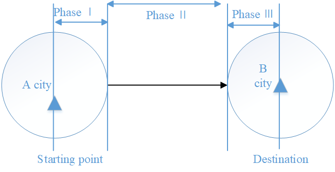
The whole process of moving residents from their point of origin to their destination is called travel. The geographical range of origin and destination can be divided into intra-city travel and inter-city travel. Intercity travel refers to whole process of residents moving in one direction from one city to another city via an intercity transportation channel in order to achieve a certain purpose of life and production. The diagram is shown in Figure 1:
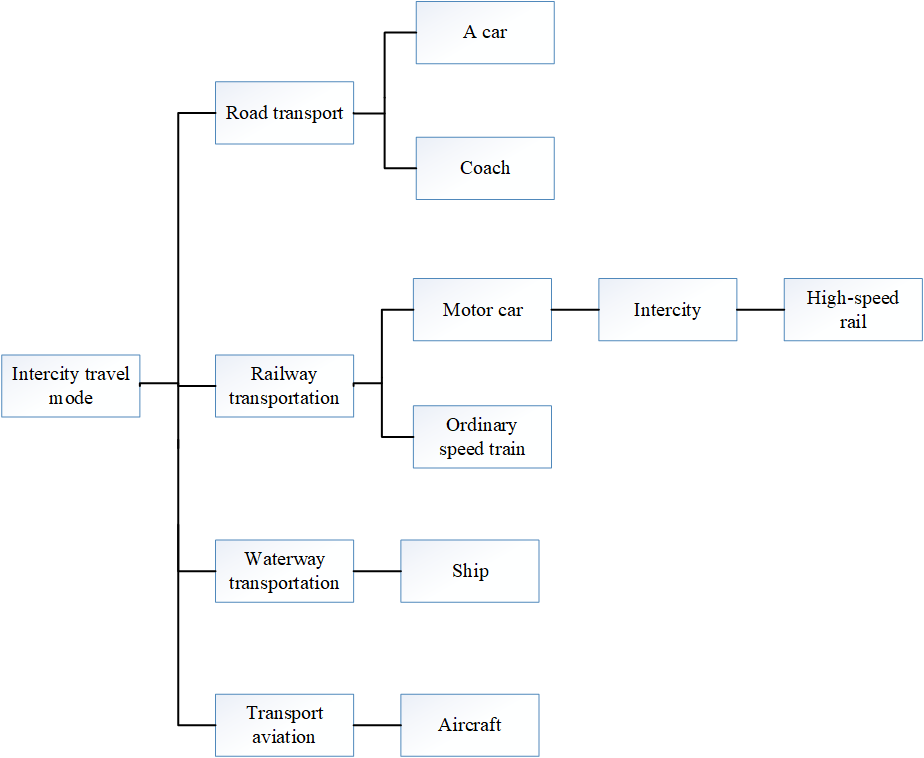
Intercity travel mode choice, as an important part of intercity travel behavior decision, also has a mutual influence with other choice links. This is mainly because different intercity travel modes differ in their own characteristics and applicable conditions, which are reflected in departure time, travel time consumption, and route. The types of intercity travel modes are divided into following categories as shown in Figure 2.
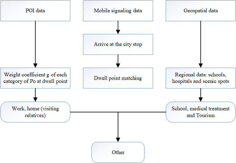
This paper classifies travel purposes into six categories based on ability and characteristics of fused data: home (including visiting relatives), work, school, medical, travel and others. In order to improve accuracy of travel purpose recognition, most suitable recognition method is chosen for different travel purposes. The three travel purposes of school, medical treatment and tourism are extracted by stopping point matching method; two travel purposes of home (visiting relatives) and work are extracted by POI weighting method. The travelers who are not in above five travel purposes are judged to be other travel purposes. The flow chart of travel purpose extraction is shown in Figure 3:
The prediction model of xgboost can be expressed as:
\[\label{e1} {\hat y_i} = \sum\limits_{k = 1}^K {{f_k}} \left( {{x_j}} \right),\tag{1}\] where, K – total number of carts; \({f_k}\) – kth cart,Characteristic vector corresponding to \({{x_j}}\) -sample I, \({\hat y_i}\)– prediction results of sample I.
After getting model, we need to solve model. Balancing algorithm performance and operation speed is art of machine learning, so it is particularly important to solve model objective function. Xgboost uses traditional loss function + model complexity as solution objective, which can be written as following formula:
\[\label{e2} {\text{ obj }} = \sum\limits_{i = 1}^n l \left( {{y_i},{{\hat y}_i}} \right) + \sum\limits_{k = 1}^K \Omega \left( {{f_k}} \right),\tag{2}\] where: n – total amount of data imported into kth cart, \(l\left( {{y_i},{{\hat y}_i}} \right)\) training error of sample I, usually expressed by adjusted mean square error RMSE; \(\Omega \left( {{f_k}} \right)\) – regular term of k-th tree, representing complexity of model.
Combined with above two sets of expressions, since \({\hat y_i}\) already contains iteration results of all carts, entire objective function is related to K carts. So two parts of OB are solved respectively. For first part, in process of model learning, a cart is added in each iteration to fit residual between predicted value and real value obtained in last iteration. Assuming that predicted value predicted in step t is \(\hat y_i^{(r – 1)}\), expression is as follows:
\[\label{e3} \hat y_i^{(0)} = 0.\tag{3}\]
\[\label{e4} \hat y_i^{(t)} = \sum\limits_{k = 1}^l {{f_k}} \left( {{x_i}} \right) = \hat y_i^{(r – 1)} + {f_i}\left( {{x_i}} \right).\tag{4}\]
With increase of cart, loss function changes. When t-th cart is established, first T1 carts have been trained, and second term in objective function and training error have become known constant terms. Using Taylor expansion, objective function can be transformed into:
\[\label{e5} obj = \sum\limits_{i = 1}^n {\left[ {l\left( {{y_i},{{\hat y}^{(t – 1)}}} \right) + {g_i}{f_i}\left( {{x_i}} \right) + \frac{1}{2}{h_i}f_t^2\left( {{x_i}} \right)} \right]} + \Omega \left( {{f_t}} \right) + C,\tag{5}\] where: \(l\left( {{y_i},{{\hat y}^{(t – 1)}}} \right)\) – training error obtained from 11 cart is a constant: \({g_i}\) – first derivative of loss function \(l\left( {{y_i},{{\hat y}^{(t – 1)}}} \right)\) to \({\hat y^{(t – 1)}}\), \({h_i}\) – second derivative of loss function \(l\left( {{y_i},{{\hat y}^{(t – 1)}}} \right)\) to \({\hat y^{(t – 1)}}\).
So far, xgboost is an integration algorithm based on gbdt, and integration relationship between carts has been solved. G and H are only related to traditional loss function. Next, we need to solve (x) of each cart, that is, regular term part of objective function, which can be expressed as:
\[\label{e6} {f_i}(x) = {\omega _{q(x)}},\tag{6}\] where: \(\omega\) -leaf node score value \(\omega \in {R^T}\) , \(q\left( x \right)\) – leaf node corresponding to sample x. Thus, when L2 regularization is adopted, second term representing complexity in objective function can be expressed as:
\[\label{e7} \Omega \left( {{f_i}} \right) = \gamma T + \frac{1}{2}\lambda \sum\limits_{j = 1}^r {\omega _j^2} ,\tag{7}\] where: t is number of leaf nodes;J-index of each leaf node \({\omega _j}\) -Weight of a leaf node with index J:Y-A super parameter that controls number of leaves;A parameter that controls intensity of regularization. Ll regularization uses a.
Replace above formula back to objective function \(obj\left( \theta \right)\) and sort it out to get:
\[\label{e8} {\operatorname{obj} ^{(t)}} = \sum\limits_{j = 1}^T {\left[ {{G_j}{\omega _j} + \frac{1}{2}\left( {{H_j} + \lambda } \right)\omega _j^2} \right]} + \gamma T,\tag{8}\] where, \({G_j} = \sum\limits_{i \in {I_j}} {{g_i}} ,{H_i} = \sum\limits_{i \in {I_j}} {{h_i}}\).
It is defined that each value of J is a quadratic function \({\omega _j}\) with \({F^*}\left( {{\omega _j}} \right)\) as independent variable. In order to minimize objective function \({\operatorname{obj} ^{(t)}}\), as long as quadratic function under value of J of each leaf is smallest, sum must also be most.
\[\label{e9} {F^*}\left( {{\omega _j}} \right) = {\omega _j}{G_j} + \frac{1}{2}\omega _j^2\left( {{H_j} + \lambda } \right).\tag{9}\]
So, on \({F^*}\left( {{\omega _j}} \right)\), \({\omega _j}\), Find derivative, make first derivative equal to 0, find extreme value, and you can get:
\[\label{e10} {\omega _j} = – \frac{{{G_j}}}{{{H_j} + \lambda }}.\tag{10}\]
If above formula is substituted into objective function, there are:
\[\label{e11} ob{j^{(t)}} = – \frac{1}{2}\sum\limits_{j = 1}^T {\frac{{G_j^2}}{{{H_j} + \lambda }}} + \gamma T.\tag{11}\]
So far, compared with original loss function + complexity, objective function has been transformed, and sample size I has been attributed to each leaf. Further, in order to find best branch of cart, that is, difference of structural scores, we can use basic principle of cart solution, that is, using greedy algorithm to control local optimization to achieve global optimization. Since cart is all binary tree, difference of structure scores after branching can be expressed as:
\[\label{e12} {\text{ Gain }} = \frac{1}{2}\left[ {\frac{{G_L^2}}{{{H_L} + \lambda }} + \frac{{G_R^2}}{{{H_R} + \lambda }} – \frac{{{{\left( {{G_L} + {G_R}} \right)}^2}}}{{{H_L} + {H_R} + \lambda }}} \right] – \gamma ,\tag{12}\] where: \({G_L}\) , \({H_L}\) – respectively represent sum of first and second derivatives of loss function at left node; \({H_R}\) ,\({G_R}\) and h- respectively represent sum of first and second derivatives of loss function at right node.
For each layer of each cart, above formula is calculated. Compared with original gradient descent, practice has proved that this method for solving optimal tree structure is faster and performs well on large data sets. Based on understanding of principle of X gboost model, more attention is paid to design of xgboost parameters in actual modeling and application process. Due to complexity of model, many parameters are involved, some of which are.
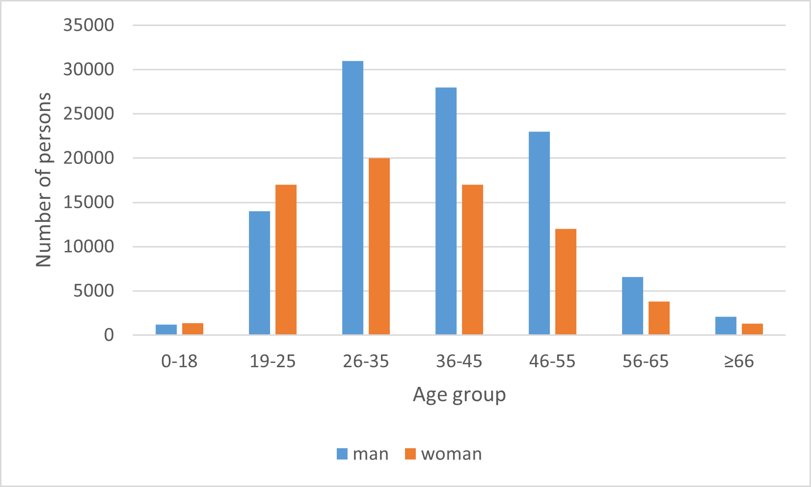
Since age and gender are important attributes for intercity travel behavior analysis, personal basic information contained in cell phone data is incomplete due to information collection and other factors, so such users should be deleted. Among 195,627 intercity travelers, 18,934 users remained after deleting those with null values of gender and age and those with less than 200 daily signaling data. The age-sex distribution of target group is shown in Figure 4:
In this paper, we take Chengdu – Mianyang intercity trip as an example, and distribution of departure time and arrival time of intercity trip intercity section after segmentation is shown in Figure 5:
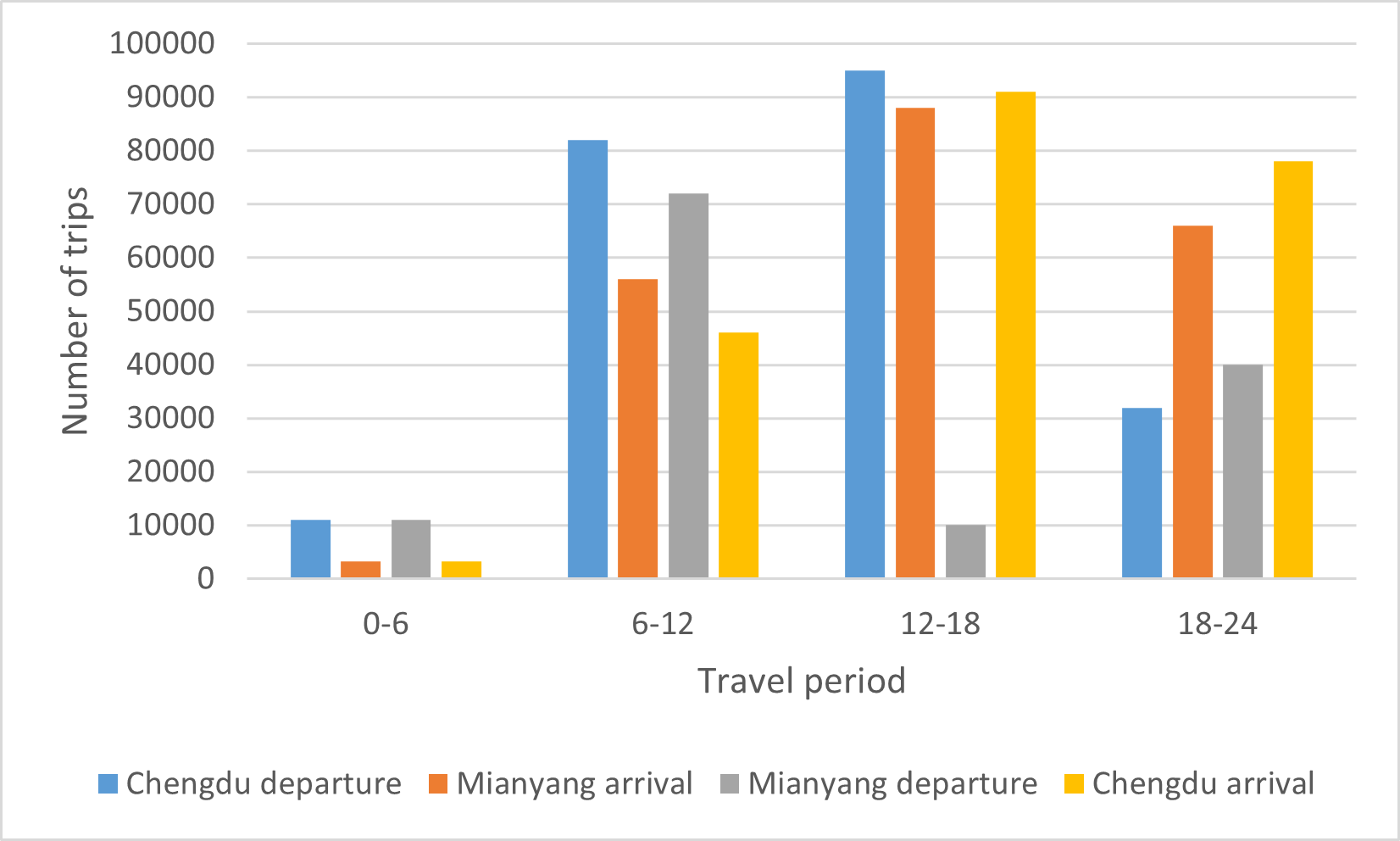
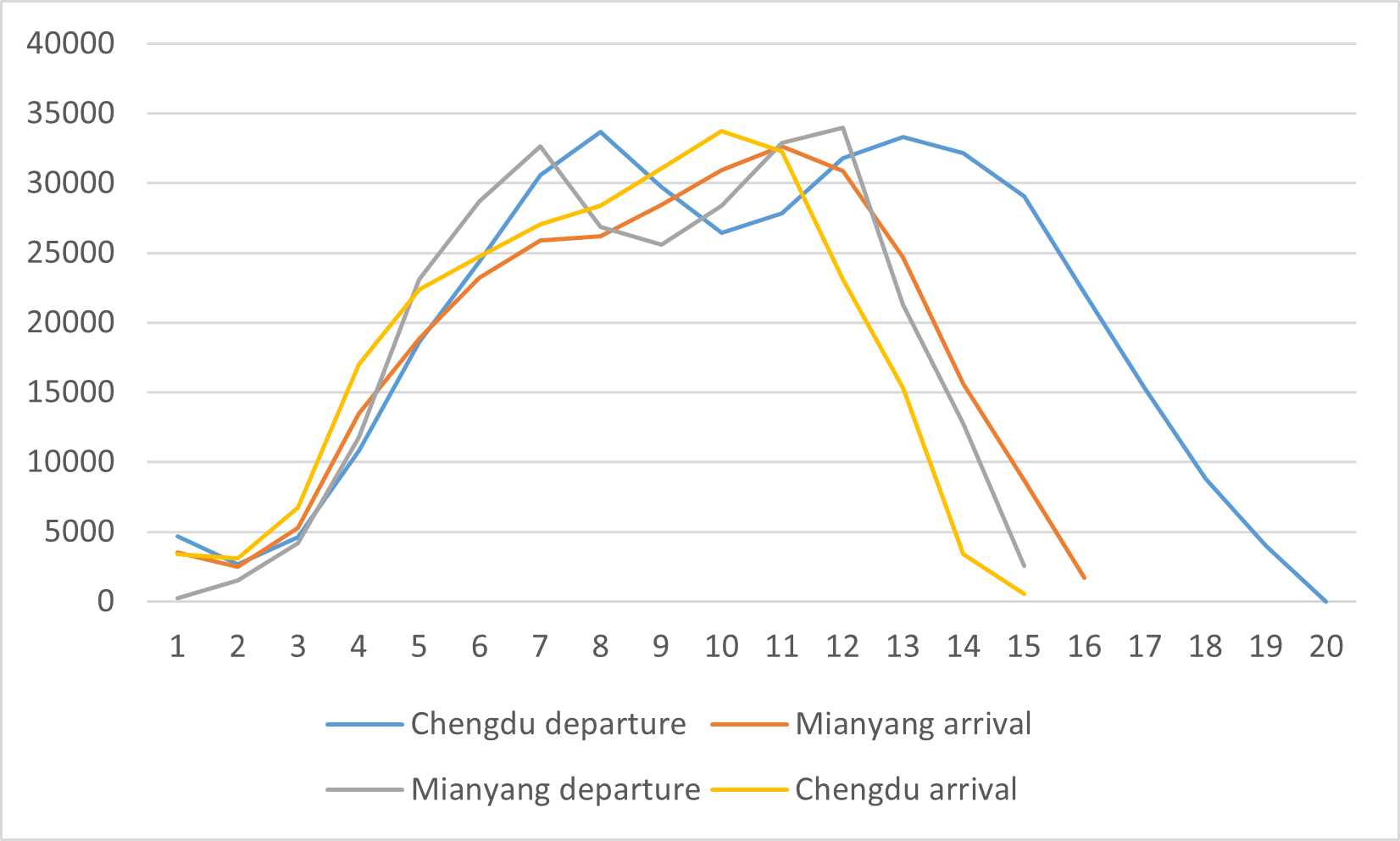
From Figure 5 above, it can be seen that intercity travel activity is weakest between 0:00 and 6:00, mainly because this time is usually people’s rest time, which is in line with common sense. A finer granularity (as shown in Figure 6) shows that there is a double-peak characteristic of Chengdu-Miandu intercity travel, but it is not obvious, for example, departure peak is from 8:00 to 10:00 and 14:00 to 16:00 in Chengdu, arrival peak is from 10:00 to 12:00 in Mianyang, departure peak is from 16:00 to 18:00 in Mianyang, and arrival peak is from 18:00 to 20:00 in Chengdu, and this delay characteristic is generally consistent with travel time of Chengdu-Miandu intercity travel. This delay characteristic is generally consistent with travel time of Chengdu-Miandu Intercity. Common sense shows that departure and arrival time characteristics of Chengdu-Miandu intercity travel are different from those of regular intra-city travel, mainly in terms of double-peak characteristics and delay of peak hours.
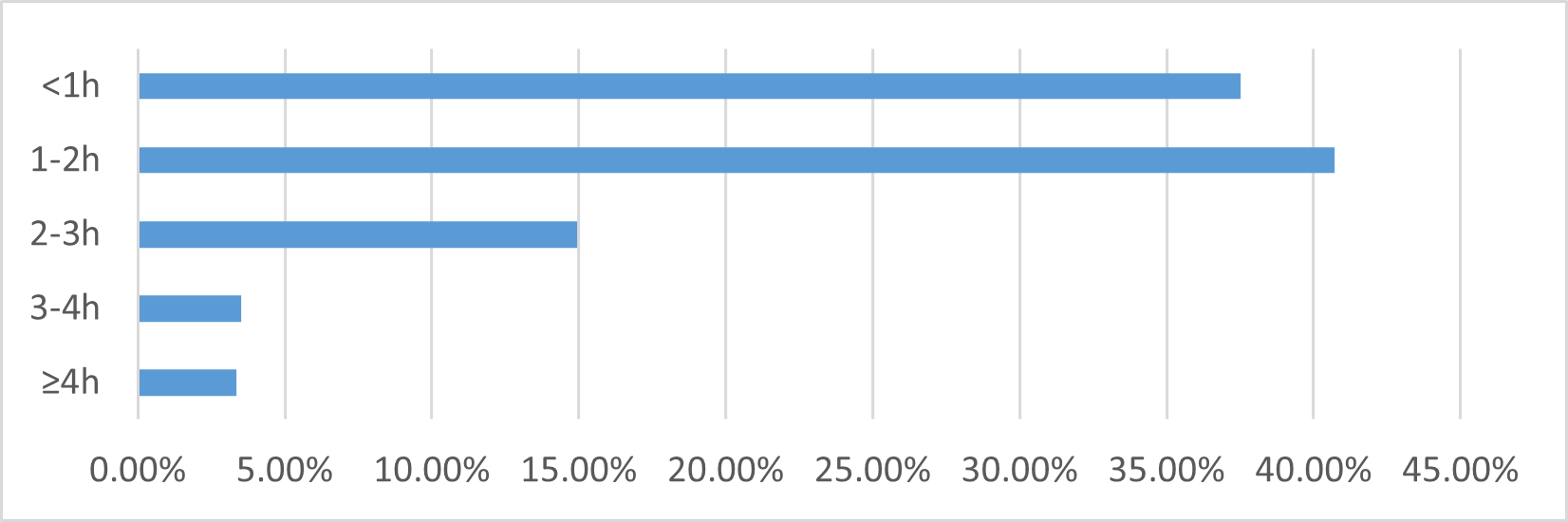
Since travel in intra-city section is limited by travel distance, for example, in Chengdu and Mianyang, it can usually be completed within 2 h. Therefore, distribution of departure and arrival times in intra-city section is not as characteristic as that in inter-city section, so it is not shown again. However, travel time of each section can be obtained intercity section and difference between arrival time and departure time of intracity section, which is an important feature affecting choice of intercity travel mode:
As can be seen from Figure 7 above, intercity section of Chengmian intercity travel has highest percentage of travel time of 1 to 2 hours, reaching 40.7%; followed by less than 1 hour, accounting for 37.52%; travel time of 2 to 3 hours accounts for 14.94%; proportion of more than 3 hours is very small, only 6.84%. Such travel time data distribution is closely related to distance and traffic conditions of Cheng-Mian intercity, on other hand, travel time of intercity section is also a major attribute of intercity travel mode, which has a great influence on choice of intercity travel mode of intercity travelers.
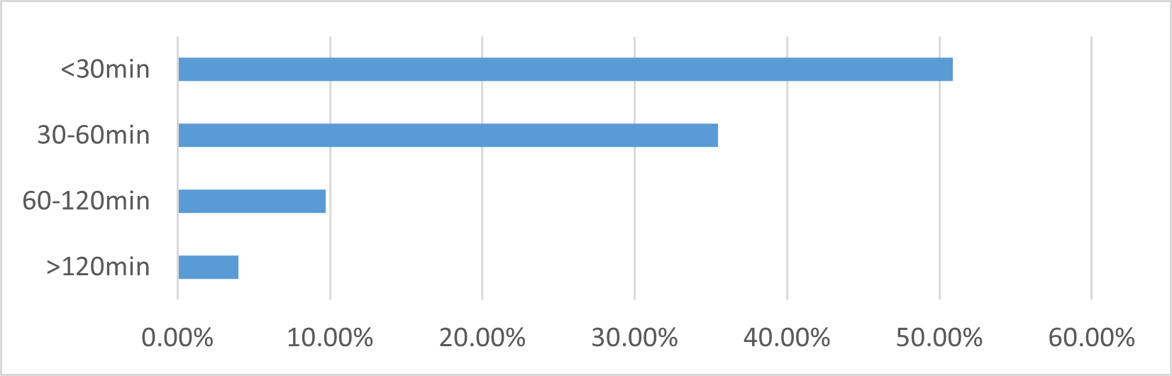
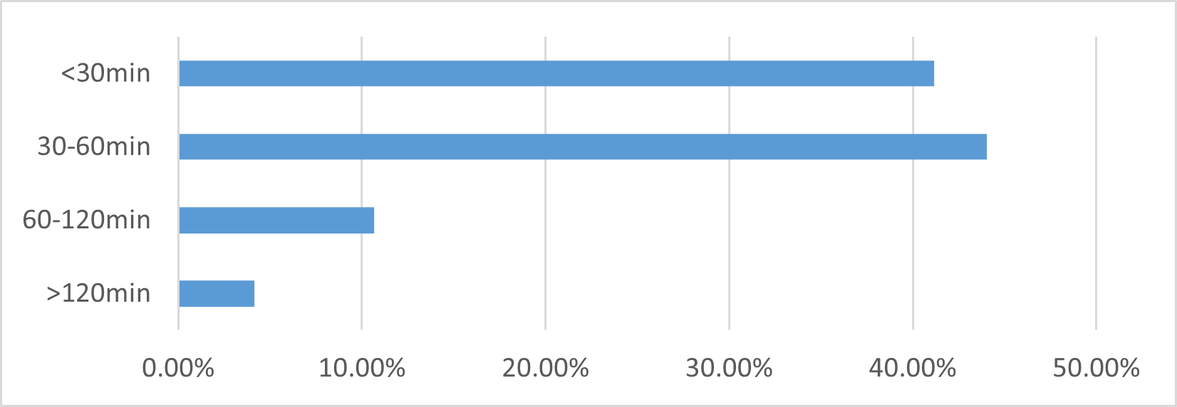
This is mainly related to travel distance, which is generally smaller than intercity section, so travel time is relatively less. The highest percentage of travel time in city section is less than 30 minutes, which is 50.87% (Figure 8). The arrival time was different, with highest percentage of arrival time between 30 and 60 minutes (44.04%). The reason for this result may be that intercity travelers are more unfamiliar with traffic environment in arrival city than in departure city, so they spend more time traveling in inner city section of arrival city than in departure city (Figure 9). Of course, this may also be related to traffic conditions of departure city and arrival city itself, and city level [5]. For example, compared with Mianyang, transportation system in Chengdu is more complete, which will have a positive impact, but city has a larger area, and travel time may increase with increase of travel distance, which will have a negative impact. Therefore, for study of intercity travel mode choice behavior, it is necessary to model each intercity trip for each individual traveler to analyze how travel time in inner city section affects intercity travel mode choice.
During study period, among four modes of travel in Chengdu-Miannan intercity section, largest number of trips were made by cars, accounting for 47.31% of trips, followed by trains, accounting for 38.28% of trips, and 12.59% of trips were made by regular trains, while smallest number of trips were made by coaches. Among railroad travel modes, number of people who choose train as intercity travel mode is about three times of those who choose general speed train. Among road travel modes, number of people who choose cars as intercity travel mode is much higher than that of coaches. The statistics on number of trips taken by four intercity travel modes are shown in Table 1:
| – | Direction / method / date | 11.04 | 11.05 | 11.06 | 11.07 | 11.08 | 11.09 | 11.10 |
|---|---|---|---|---|---|---|---|---|
| Chengdu | Acar | 6254 | 6213 | 6254 | 6258 | 8471 | 8623 | 7785 |
| Chengdu | Coach | 142 | 157 | 151 | 151 | 198 | 174 | 178 |
| Mianyang Chengdu | Ordinary speed train | 1478 | 1479 | 1354 | 1657 | 2741 | 2284 | 2536 |
| Mianyang Chengdu | Mtor train unit | 4814 | 4157 | 4213 | 4789 | 8321 | 7048 | 6984 |
| Mianyang Chengdu | Acar | 6885 | 6100 | 6547 | 7024 | 8974 | 8120 | 10057 |
| Mianyang Coach | 321 | 254 | 301 | 328 | 587 | 421 | 625 | |
| Mianyang Coach | Ordinary speed train | 1745 | 1432 | 1587 | 1625 | 2478 | 25471 | 2671 |
| Mianyang Coach | Mtor train unit | 4854 | 4662 | 4578 | 5213 | 5289 | 7457 | 7120 |
According to purpose extraction algorithm, intercity users’ intercity travel purpose is extracted by fusing Chengmian cell phone signaling data, POI data and geospatial data. The purpose of travel refers to reason why intercity travelers make intercity travel. In this paper, intercity travel purposes of Chengmian intercity travelers are divided into six types, namely, going home (or visiting relatives), work, school, tourism, medical treatment and others. The number of trips for different intercity trip purposes is shown in Table 2:
| Destination /date | 11.04 | 11.05 | 11.06 | 11.07 | 11.08 | 11.09 | 11.10 |
|---|---|---|---|---|---|---|---|
| Get home | 4925 | 4874 | 4947 | 5214 | 7451 | 7126 | 6574 |
| Work | 5231 | 3578 | 3652 | 3784 | 5471 | 3625 | 4952 |
| Go to school | 295 | 293 | 287 | 320 | 457 | 423 | 254 |
| Travel | 1817 | 1874 | 1859 | 1924 | 2745 | 1658 | 2471 |
| Seek medical advice | 332 | 357 | 287 | 365 | 354 | 332 | 374 |
| Other | 1421 | 1429 | 1475 | 1456 | 2137 | 2087 | 1954 |
From Table 2 above, it can be seen that, among intercity trips in direction of Chengdu → Mianyang during study period, largest number of trips were made for purpose of going home (or visiting relatives), followed by work [3]. In terms of time trends, intercity travel for purpose of going home (or visiting relatives) peaked on November 8 (Friday); travel for purpose of work peaked three times during week, namely on November 4 (Monday), November 8 (Friday) and November 10 (Sunday). Intercity travel for tourism purposes peaks on weekends, but peak characteristics are not obvious. The proportion of trips with school and medical purposes as intercity trips is low.
As shown in Table 3 above, intercity trips in direction of Mianyang-Chengdu with purpose of going home (or visiting relatives) or working show similar characteristics as those in direction of Chengdu-Miangyang. However, number of intercity trips witnessed by medical treatment has increased, which is probably due to fact that Chengdu, as capital of Sichuan Province, has better medical resources than Mianyang City.
In terms of XGBoost model prediction evaluation index (Table 4) and running time (Table 5), XGBoost has excellent prediction results on test dataset, with a prediction accuracy of 95.55%, a fl value of 95.46%, and a running time of 453.79 s. Overall, model has excellent prediction ability, with highest prediction accuracy for small cars and lowest prediction accuracy for a few types of coaches. The model has highest prediction accuracy for small cars and lowest prediction accuracy for a few types of coaches. From principle of XGBoost, it can be seen that running time of XGBoost is long because model builds a tree model based on gradient descent, and there are correlations between trees [2].
| Destination /date | 11.04 | 11.05 | 11.06 | 11.07 | 11.08 | 11.09 | 11.10 |
|---|---|---|---|---|---|---|---|
| Get home | 5355 | 5302 | 5321 | 2625 | 8147 | 7852 | 7232 |
| Work | 5781 | 3857 | 3925 | 4127 | 5998 | 3924 | 5321 |
| Go to school | 321 | 320 | 328 | 339 | 487 | 469 | 445 |
| Travel | 1982 | 1963 | 1995 | 2087 | 3017 | 2887 | 2714 |
| Seek medical advice | 980 | 825 | 1057 | 709 | 968 | 935 | 984 |
| Other | 1550 | 1532 | 1657 | 2365 | 2258 | 2118 | 2471 |
| Actual forecast | A car | Coach | Ordinary speed train | Motor train unit |
|---|---|---|---|---|
| A car | 3015 | 0 | 0 | 815 |
| Coach | 0 | 880 | 205 | 432 |
| Ordinary speed train | 0 | 0 | 8351 | 234 |
| Motor train unit | 1210 | 0 | 370 | 2398 |
| Evaluating indicator | Accuracy | F1 value | Running time |
|---|---|---|---|
| Value | 0.956 | 0.955 | 454.78 |
In this paper, intercity travel mode selection behavior is studied based on machine learning methods by integrating cell phone signaling data, geospatial data, and POI data in the context of big data. Based on the analysis of influencing factors of intercity travel mode selection behavior, we designed a data pre-processing method including cell phone signaling data, geospatial data, and POI data, as well as an intercity travel feature data extraction algorithm including target group, travel chain, travel mode, and travel purpose. We constructed an intercity travel mode selection model based on the XGBoost machine learning method, and combined with an example, we verified intercity travel feature data using railway ticket data. The effectiveness of the intercity travel feature data extraction algorithm is verified by using railroad ticket data, and the advantages and disadvantages of three models are compared and analyzed based on the accuracy of model prediction results and running time.
Additionally, the findings from this study have significant implications for higher education in tourism talent cultivation. Incorporating such advanced data analytics and machine learning methodologies into academic curricula can enhance the theoretical and practical knowledge of tourism students. Core courses like tourism economics and management can integrate case studies on data-driven decision-making in travel behavior analysis. Practical training sessions, including internships and simulations, can be enriched with real-world data processing and model-building exercises. Encouraging interdisciplinary learning and research can further prepare students for the evolving demands of the tourism industry. By fostering skills in data analysis, machine learning, and geospatial technologies, higher education institutions can better equip future professionals to address complex challenges in travel and tourism management.
The authors would like to show sincere thanks to those techniques who have contributed to this research.
All authors reviewed the results, approved the final version of the manuscript and agreed to publish it.
The experimental data used to support the findings of this study are available from the corresponding author upon request.
The authors declared that they have no conflicts of interest regarding this work.
This study by funding support:Humanities and Social Science Research Project of Hebei Education Department(No:BJS2023032); Hebei Northern University 2023 Innovation and Entrepreneurship School-Level Education and Teaching Reform Research and Practice Project: Research on the Construction of an Educational Ecosystem for Innovation and Entrepreneurship Research in Colleges and Universities under the Background of High-Quality Development Hebei Northern University Education and Teaching Reform Research Project, Research on the Path and Countermeasures of Improving the Practical Ability of Hotel Management Students through the Integration of Competition and Education Based on CIPP Evaluation(JG202227); Hebei Northern University Education and Teaching Reform Research Project, Empowering Learning, Competition and Research, and Connecting the Industrial Chain: Improving and Rebuilding the Practical Teaching of Hotel Management Majors under the Background of New Liberal Arts (JG2024008).