
The plateau vortex, a sub-weather-scale low-pressure vortex that occurs on the main body of the plateau in summer and half a year, is a major weather system in the plateau region [5, 26]. It is often generated in the central and western part of the plateau, and most of it weakens and disappears in the downslope of the eastern part of the plateau, rarely moving out of the plateau, and is the main rainfall system on the plateau in summer [7,17,25]. It is worth noting that, under the favorable circulation situation, individual plateau vortex can move eastward out of the plateau development, often triggering the downstream area of the plateau a wide range of heavy rain, thunderstorms and other catastrophic weather processes [13,23].
Atmospheric circulation refers to the distribution and movement of various meteorological elements in the atmosphere in the horizontal and vertical directions, including air pressure, temperature, humidity, wind direction and wind speed. It is an indispensable part of the earth’s climate system and plays an important role in the formation and change of the earth’s climate [14,20,22,3]. Atmospheric circulation is mainly divided into two categories, one is global atmospheric circulation and the other is local atmospheric circulation. The global atmospheric circulation refers to the extensive movement of the Earth’s atmosphere, including the equatorial low-pressure belt, subtropical high-pressure belt, polar low-pressure belt, and North and South Polar high-pressure systems and other components of the circulation system [1,6,16,21]. This circulation system is the result of a combination of factors such as the Earth’s rotation, solar radiation, and temperature differences between different regions of the Earth’s surface [19,11,10]. Local atmospheric circulation refers to the movement of air currents in local areas on the Earth, including local winds, ocean winds, topographic winds and valley winds. This circulation system is the result of the combined effect of factors such as topography, sea and land distribution, surface cover, solar radiation, etc. [9,15,18].
This paper proposes an adaptive filtering algorithm to analyze the data related to the plateau vortex and atmospheric circulation, adjust and optimize the filtering coefficients in the filtering subsystem through the adaptive algorithm module, and realize the adaptive adjustment of the filtering step size of the adaptive filtering algorithm. The basic Wiener filter structure is then used to separate the signal from the noise of the plateau vortex and atmospheric circulation data, so as to optimize the performance of the adaptive filtering algorithm in data processing. Subsequently, this paper introduces the LMS criterion into the adaptive filtering algorithm for further optimization, and proposes the quantization error algorithm and the affine projection algorithm to deal with the ordinary data and the strong correlation data, so as to reduce the data analysis error and convergence speed of the adaptive filtering algorithm. In this study, the performance of the adaptive filtering algorithm optimized based on the LMS criterion is tested by experimentally analyzing the noise covariance and online filtering performance of the algorithm in data processing. The coupling effect and spatial and temporal characteristics of the vortex and atmospheric circulation over the Tibetan Plateau during the period of 2000-2020 are investigated by using the data of the vortex and atmospheric circulation over the Tibetan Plateau.
1) Random signals, arbitrary in the system, with no clear connection to time, in a state of disorder, can not be described by an accurate time function of the signal, but, in this chaotic world, the value of the change is subject to statistical laws.
2) Deterministic signals, can be used as a function of time, graphical representation of the signal for deterministic signals, that is, given a time series \(t\), can predict the size of the \(y=x\left(t\right)\) signal for deterministic signals.
The filtering subsystem and the adaptive algorithm module [8] are the main building blocks of the adaptive filter. The filter subsystem, which is one of the key components of the system, is characterized by a variety of structural modes depending on the function it solves. The adaptive algorithms are at the heart of the filter computation, where the adjustment of the filter coefficients or of the parameters of the filter sub-structure is done in the algorithmic part. Various criteria and algorithms intervene during the adjustment of the adaptive filter coefficients. The focus of the algorithmic tuning is the adaptive tuning of the filtering step size, which aims at a rapid decrease of the error to a global minimum in accordance with the principles set by the system. The adaptive process I and the filtering process II are the two processes in the filtering part of the adaptive filter. Adjustment of the filter coefficients \(w_{i} (k)\) is the fundamental goal of process 1, which results in a gradual decrease of the useful objective function \(\varepsilon \left(\cdot \right)\) and a gradual approximation of the signal \(y(k)\) to the desired reference signal \(d(k)\), which is used as the final output. The adjustment principle of filter coefficients is mainly carried out by the error signal \(e(k)\) between \(y(k)\) and \(d(k)\) to carry out a certain algorithm, the result of which allows the filter to quickly be in the optimal working condition, and ultimately complete the filtering goal. It can be seen that the adaptive algorithm process is an iterative search for the global optimum, and the regulation mechanism of the algorithm affects the time required for the adaptive process in the iterative loop \(t\). It should be noted that the objective function \(\varepsilon \left(\cdot \right)\) is a function of \(x(k)\), \(d(k)\), and \(y(k)\), i.e., \(\varepsilon \left(\cdot \right)=\varepsilon \left[x(k),d(k)y(k)\right]\), and therefore the objective function should have two properties.
1) Non-negativity: \[\label{GrindEQ__1_} \varepsilon \left(\cdot \right)=\varepsilon \left[x(k),d(k),y(k)\right]\ge 0,\forall x(k),d(k),y(k) .\tag{1}\]
2) Optimality: \[\label{GrindEQ__2_} \varepsilon \left(\cdot \right)=\varepsilon \left[x(k),d(k),y(k)\right]=0,{\rm \; }when{\rm \; }y(k)=d(k) .\tag{2}\]
Adaptive parameter optimization process, the essence of the corresponding algorithm to make the objective function \(\varepsilon \left(\cdot \right)\) gradually minimized, finally, can make \(y(k)\) infinitely close to the signal \(d(k)\), can make the parameters in the system \(w_{i} (k)\) converge to \(w_{opt}\), this solution \(w_{opt}\) is the best solution of the parameters of the adaptive algorithm. Thus, the adaptive adjustment process is the optimal linear expected adaptive adjustment process, in order to facilitate the adjustment of the main objective direction, at this time, both the filter is expected to complete the desired signal \(d(k)\), and the weight coefficients are expected to be adjusted, the two should be considered at the same time, and this successive time-varying form of the analysis occurs throughout the process.
A filtering technique that separates useful signals from the noise of plateau eddy and atmospheric circulation data is the Wiener filtering technique. Stable stochastic process models and degenerate models of linear spatially robust systems are its theoretical basis. As a requirement for the design of Wiener filter, i.e., to give a representation of the \(h(k)\) or \(H(z)\) function of the filter under the condition of minimum mean-square error, the essence of the process is to solve the Wiener-Hopf equation. \(x(k)\) and \(y(k)\) signals are fed into the filter at the same time in the conventional Wiener filter structure [4]. The mathematical model \(y(k)\) will contain a connected component in \(x(k)\), while the other component is independent of \(x(k)\). The Wiener filter generates an optimal prediction of the connected component with \(x(k)\) in \(y(k)\), while \(e(k)\) is obtained by subtracting \(y(k)\) from this analysis.
If there is a FIR filter consisting of \(N\) weight coefficients, the Wiener filter is \(e(k)\) differentiated from the original signal \(y(k)\) and the result is: \[\label{GrindEQ__3_} e_{k} =y_{k} -\hat{n}_{k} =y_{k} -w^{T} x_{k} =y_{k} -\sum _{i=0}^{N-1}w (i)x_{k-i},\tag{3}\] where \(x_{k}\) and \(w\) are the input signal vector and weight vector, respectively, determined by: \[\label{GrindEQ__4_} x_{k} =\left[\begin{array}{l} {x_{k} } \\ {x_{k-1} } \\ {M} \\ {x_{k-(N-1)} } \end{array}\right],\quad w=\left[\begin{array}{l} {w(0)} \\ {w(1)} \\ {M} \\ {w(N-1)} \end{array}\right] .\tag{4}\]
The error squared is: \[\label{GrindEQ__5_} e_{k}^{2} =y_{k}^{2} -2y_{k} x_{k}^{T} w+w^{T} x_{k} x_{k}^{T} w .\tag{5}\]
The mean square error \(\left(MSE\right)\varepsilon\) can be obtained by taking the expectation around the Eq. (5), if \(x(k)\) and \(y(k)\) as the afferent and efferent are combined with the ansatz, that is: \[\begin{aligned} \label{GrindEQ__6_} {\varepsilon } {=} & {E\left[e_{k} \right]^{2} } \notag\\ {} {=} & {E\left[y_{k} \right]^{2} -2E\left[y_{k} x_{k}^{T} w\right]+E\left[w^{T} x_{k} x_{k}^{T} w\right]} \notag\\ {} {=} & {\sigma ^{2} +2P^{T} w+w^{T} Rw}, \end{aligned}\tag{6}\] where \(E\) represents the expectation, \(\sigma ^{2} =E\left[y_{k} \right]^{2}\) is the variance of \(y(k)\), \(P=E\left[y_{k} x_{k} \right]\) is the inter-correlation vector of length \(N\), and \(R=E\left[x_{k} x_{k}^{T} \right]\) is the autocorrelation matrix of \(N\times N\). The graph obtained from the filter coefficients of a bowl-shaped MSE is characterized by a unique minimum bottom whose values are all greater than zero. The gradient of the altered graph surface can be expressed as: \[\label{GrindEQ__7_} \nabla =\frac{d\varepsilon }{dw} =-2P+2Rw .\tag{7}\]
In weighting coefficient \(w(i)\), the coefficients self correspond to points in the surface, in the lowermost part of the surface, when the gradient vector obtains very small, and the filtering weight vector approaches the optimal \(w_{opt}\): \[\label{GrindEQ__8_} w_{op} =R^{-1} P .\tag{8}\]
This is the solution of the Wiener-Hoff equation. Appropriate algorithms are used to tune the filter weight coefficients is the first task of this algorithm \(w_{i} (0),w_{i} (1),w_{i} (2),\ldots ,w_{i} (N-1)\), so as to find the optimal point of the performance surface \(w_{opt}\).
In this paper, the adaptive filtering algorithm is optimized based on the LMS criterion [24], which aims to shorten the convergence time or reduce the complexity of the algorithm in order to improve the performance of the adaptive filtering algorithm in the analysis of spatial and temporal characteristics of the coupling effect of the plateau vortex and the atmospheric circulation. In this paper, the adaptive filtering algorithm based on the LMS criterion, i.e., quantization error method and affine projection algorithm, is designed.
The basic idea of the quantization error algorithm [2] is to reduce the computational complexity of the LMS algorithm by using a short word length or using a simple power of 2. The computational complexity is the multiplication operation performed during the coefficient update as well as the operation of the output signal of the adaptive filter, which simplifies the LMS algorithm by quantizing the error signal, and ultimately obtains the quantization error adaptive filtering algorithm, which has adjustable parameters the digital filter weight coefficient update equation is: \[\label{GrindEQ__9_} w(k+1)=w(k)+2\mu Q[e(k)]x(k) ,\tag{9}\] where \(Q\left[\cdot \right]\) is the quantization operation. The quantization function is a function that takes discrete values, is bounded, and is non-decreasing. Different quantization methods determine the various quantization error algorithms.
Quantization of the error implies a modification of the minimization objective function, and in gradient type algorithms, the weights are updated with the following formula: \[\label{GrindEQ__10_} {w(k+1)} =w(k)-\mu \frac{\partial F[e(k)]}{\partial w(k)} ={w(k)-\mu \frac{\partial F[e(k)]}{\partial e(k)} \frac{\partial e(k)}{\partial w(k)} }.\tag{10}\]
For linear combiners, Eq. (10) can be rewritten as: \[\label{GrindEQ__11_} w(k+1)=w(k)+\mu \frac{\partial F[e(k)]}{\partial e(k)} x(k) .\tag{11}\]
Therefore, the minimization objective function in the quantization error algorithm needs to be satisfied: \[\label{GrindEQ__12_} \frac{\partial F[e(k)]}{\partial e(k)} =2Q[e(k)] .\tag{12}\]
Common quantization error algorithms are symbol error algorithms, two-symbol algorithms, power-of-2 error algorithms, and symbol-data algorithms.
The quantization function is a symbolic function, which is defined as: \[\label{GrindEQ__13_} sgn[b]=\left\{\begin{array}{ll} {1} & {b>0} ,\\ {0} & {b=0} ,\\ {-1} & {b<0} .\end{array}\right.\tag{13}\]
The symbolic error algorithm quantifies the error using a symbolic function with an update equation for the coefficient vector: \[\label{GrindEQ__14_} w(k+1)=w(k)+2\mu sgn[e(k)]x(k) .\tag{14}\]
The idea of the two-symbol algorithm is to make large corrections to the coefficient vector when the modulus of the error signal is larger than some predetermined value. The fundamental reason for using the two-symbol algorithm is to avoid the slow convergence problem inherent in the symbolic error algorithm caused by using \(sgn\left[e\left(k\right)\right]\) instead of \(e(k)\) when \(\left|e(k)\right|\) is large.
The quantization function of the two-symbol algorithm is: \[\label{GrindEQ__15_} ds\left[a\right]=\left\{\begin{array}{ll} {\varepsilon sgn[a]} & {|a|>\rho }, \\ {sgn[a]} & {|a|\le \rho }, \end{array}\right.\tag{15}\] where \(\varepsilon >1\) is a power of 2. The two-symbol algorithm utilizes the above function to quantify the error in a way that the coefficients are updated: \[\label{GrindEQ__16_} w(k+1)=w(k)+2\mu ds[e(k)]x(k) .\tag{16}\]
The power of 2 error algorithm uses the following quantization function to quantize the error signal: \[\label{GrindEQ__17_} pe\left[b\right]=\left\{\begin{array}{cc} {sgn[b]} & {\left|b\right|\ge 1}, \\ {2^{floor} \left[\log 2^{\left|b\right|} \right]sgn[b]} & {2^{-b_{d} +1} \le \left|b\right|<1}, \\ {\tau sgn[b]} & {\left|b\right|<2^{-b_{d} +1} } ,\end{array}\right.\tag{17}\] where \(floor\left[\cdot \right]\) denotes the integer value of \(\left[\cdot \right]\), \(b_{d}\) is the word length of the data with the sign bit removed, and the \(\tau\) value is usually 0 or \(2^{-b_{d} }\).
The coefficient update equation for the power error algorithm for 2: \[\label{GrindEQ__18_} w(k+1)=w(k)+2\mu pe[e(k)]x(k) .\tag{18}\]
The data reuse method is used to improve the convergence speed of the adaptive filtering algorithm when the correlation between the signals of the plateau vortex and the coupled atmospheric circulation effects input into the adaptive filtering algorithm is high, the price paid for reusing the past signals is the increase of the algorithm’s misalignments and computational effort, so the algorithm, like ordinary algorithms, also introduces a convergence factor to balance the amount of misalignments and the speed of convergence.
In data reuse, the last \(L+1\) input vector is written as in Eq. (19), the output vector as in Eq. (20), the desired signal as in Eq. (21) and the error vector as in Eq. (22): \[ {X(k)} {=} {\left[x(k)x(k-1)\cdots x(k-L)\right]}= {\left[\begin{array}{cccc} {x(k)} & {x(k-1)} & {\cdots } & {x(k-L)} \\ {x(k-1)} & {x(k-2)} & {\cdots } & {x(k-L-1)} \\ {\vdots } & {\vdots } & {\ddots } & {\vdots } \\ {x(k-N)} & {x(k-N-1)} & {\cdots } & {x(k-L-N)} \end{array}\right]} , \tag{19}\]\[ y(k)=X^{T} (k)W(k)=\left[\begin{array}{c} {y_{0} (k)} \\ {y_{1} (k)} \\ {\vdots } \\ {y_{L} (k)} \end{array}\right] ,\tag{20}\]\[ D(k)=\left[\begin{array}{c} {d(k)} \\ {d(k-1)} \\ {\vdots } \\ {d(k-L)} \end{array}\right] ,\tag{21}\]\[ e(k)=\left[\begin{array}{c} {e_{0} (k)} \\ {e_{1} (k)} \\ {\vdots } \\ {e_{L} (k)} \end{array}\right]=\left[\begin{array}{c} {d(k)-y_{0} (k)} \\ {d(k-1)-y_{1} (k)} \\ {\vdots } \\ {d(k-L)-y_{L} (k)} \end{array}\right]=D(k)-y(k) . \tag{22}\]
The idea of the affine projection algorithm [12] is that the \(k+1\)-moment weight vector \(W(k+1)\) is kept as close as possible to the \(k\)-moment weight vector \(W(k)\), i.e., under \(D(k)-X^{{\rm T}} (k)W(k+1)=0\) conditions, to minimize the following equation: \[\label{GrindEQ__23_} \frac{1}{2} \left\| W(k+1)-W(k)\right\| ^{2} .\tag{23}\]
The transformation of an optimization problem containing constraints into a problem optimized without constraints can be achieved by using a mathematical method, i.e., the Lagrange multiplier method, where the expression of the function optimized without constraints is to minimize the following equation: \[\label{GrindEQ__24_} \begin{array}{rcl} {F[W(k+1)]} & {=} & {\frac{1}{2} \left\| W(k+1)-W(k)\right\| ^{2} } {+\lambda {}^{T} (k)\left[D(k)-X^{T} (k)W(k+1)\right]} \end{array} ,\tag{24}\] where \(\lambda (k)\) is a \((L+1)\times 1\)-dimensional Lagrange multiplier. Let \(\frac{\partial \nabla F[W(k+1)]}{\partial W(k+1)} =0\), be obtained: \[\label{GrindEQ__25_} W(k+1)=W(k)+X(k)\lambda (k) .\tag{25}\]
Bringing Eq. (25) into the constraint relationship in Eq. (23) gives: \[\label{GrindEQ__26_} X^{T} (k)X(k)\lambda (k)=D(k)-X^{T} (k)W(k)=e(k) .\tag{26}\]
The solution can be obtained from the above equation and brought into the weight update equation to get the weight update formula, in order to regulate the balance of steady state dislocation and convergence speed, the step factor is added, then the final affine projection algorithm’s weight update formula is: \[\label{GrindEQ__27_} W(k+1)=W(k)+\mu X(k)\left[X^{T} (k)X(k)\right]^{-1} e(k) .\tag{27}\]
It can be seen that the affine projection algorithm becomes a normalized least mean square algorithm when the data reuse factor is \(L=1\).
The stochastic noise characteristics of the plateau vortex and atmospheric circulation coupling effect data are usually unknown or inaccurate, and in such a scenario, the traditional Kalman filtering not only fails to play the role of noise reduction, but also destroys the beneficial signals contained in the data. Therefore, the optimized adaptive filtering method based on LMS has a good application scenario in the spatial and temporal characterization of the coupled effects of plateau eddies and atmospheric circulation. In this section, we will verify whether the adaptive filtering optimization algorithm proposed in this paper can accurately process the data related to the coupling effect of plateau vortex and atmospheric circulation, so as to ensure the analysis accuracy of the data.
In this paper, the coupled vortex and atmospheric circulation data of the Tibetan Plateau from December 4, 2023 to December 10, 2023 provided by the International Service Data Center are selected, with a sampling interval \(\mathrm{\Delta}\)t of 30s and a total of 20,512 calendar elements for seven consecutive days. The pseudorange single-point localization results are solved using RTKLIB open-source software to obtain the raw data. The data analysis performance of the three methods, SWVAKF, RT-ALS and the adaptive filtering optimization model proposed in this paper, is compared in terms of the changes of noise parameters and noise covariance of the model in the process of analyzing and processing the coupled data of the plateau vortex and the atmospheric circulation, respectively.
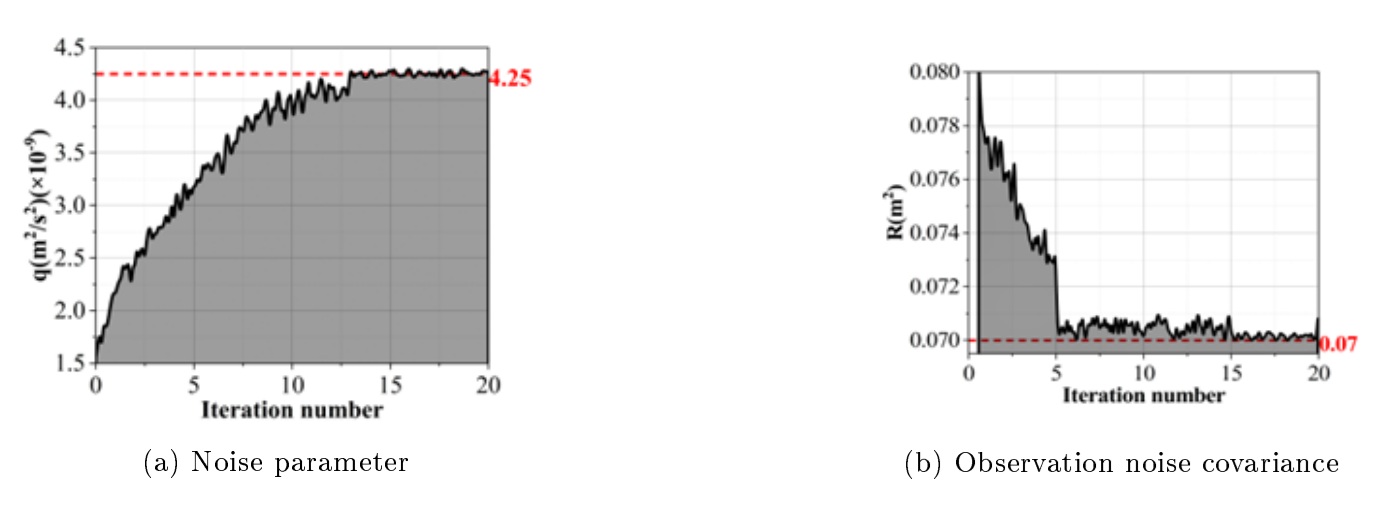
In the actual test scenario, in order to compare and analyze the data processing and analysis accuracy of the three methods, this paper takes the analysis results of the standard method ALS as the reference value of the model, and the closer the noise parameter and covariance in the data analysis processing of the model are to the reference value, which indicates that the analysis of the data of coupling of the plateau vortex with the atmospheric circulation and the analysis accuracy are more precise.The iterative results of the analysis of the ALS model are shown in Figure 1, with the changes of the noise parameter and observation noise covariance R in Figure 1 and the results of 20 iterations of the ALS model converged. Figures 1a and 1b are the results of the variation of the noise parameter and the observed noise covariance, respectively. 20 iterations of the ALS model results in the convergence of the process noise parameter q and the observed noise covariance R. Therefore, the optimal noise covariance of the ALS model is the same as the process noise parameter. Therefore, the optimal reference value of the noise covariance is q = 4.25\(\times {\rm 10}^{-9} m^{2} /s^{2}\), R = 7.00\(\times {\rm 10}^{-2} m^{2}\).
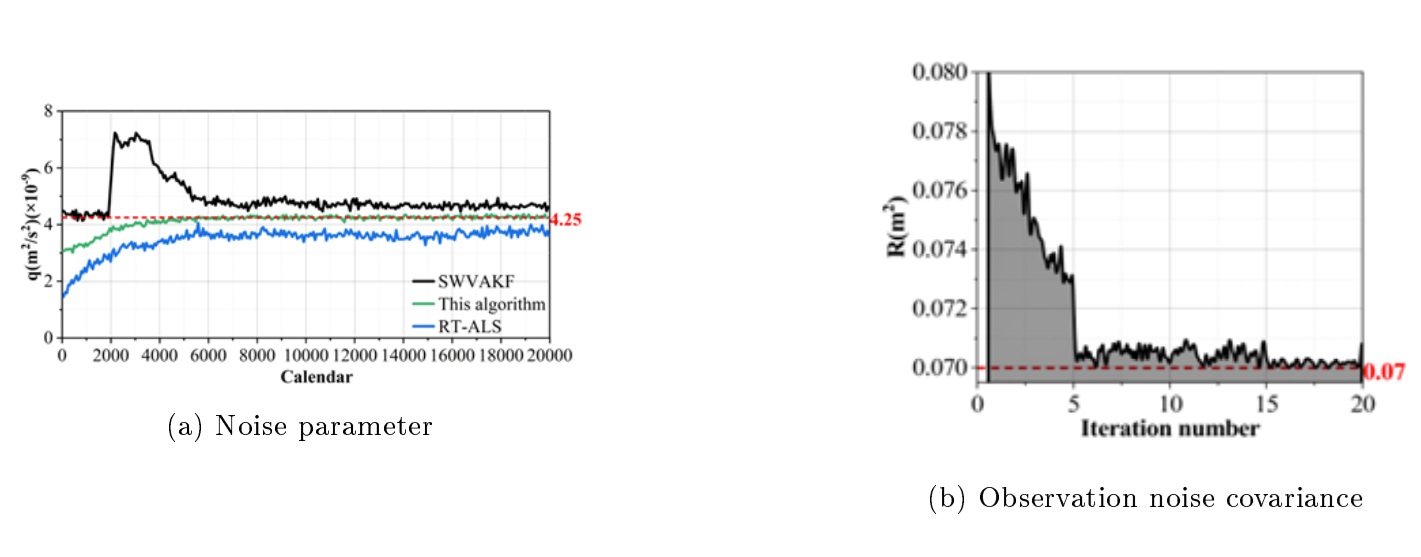
The data analysis and processing results of SWVAKF, RT-ALS and the adaptive filtering optimization algorithm proposed in this paper are shown in Figure 2, with 2a and 2b representing the results of noise and noise covariance analysis for different models, respectively. From the figure, it can be seen that the analysis results of the process noise parameter q of the SWVAKF model are unstable, and there is a large deviation from the ALS around the 2000th calendar year, which indicates that the SWVAKF model is not ideal for this process noise covariance analysis that satisfies a specific matrix form.The analysis results of the observation noise covariance R of the SWVAKF model are jittered near the ALS, and the magnitude of the jitter is less than the RT-ALS algorithm. In contrast, the analytical results of the process noise parameter q and the observed noise covariance R of the adaptive filtering optimization algorithm proposed in this paper are gradually smooth with the increase of calendar elements, and the analytical results are close to those of ALS.
In order to evaluate the online filtering analysis accuracy of different models, this paper takes the square root of the normalized Frobenius parameter of the noise covariance matrix (SRNFN) as an evaluation criterion, defined as:
\[\label{GrindEQ__28_} SRNFN=\left(\frac{1}{{\rm n}_{p}^{2} M} \sum _{s-1}^{M}\left\| \widehat{P}^{j} -\widetilde{P}^{j} \right\| ^{2} \right)^{\frac{1}{4} } ,\tag{28}\] where \(n_{p}\) denotes the dimension of the noise covariance matrix, and \(\widehat{P}^{j}\) and \(\widetilde{P}^{j}\) are the valuation and truth value of the noise covariance matrix at the jth Monte Carlo simulation, respectively.
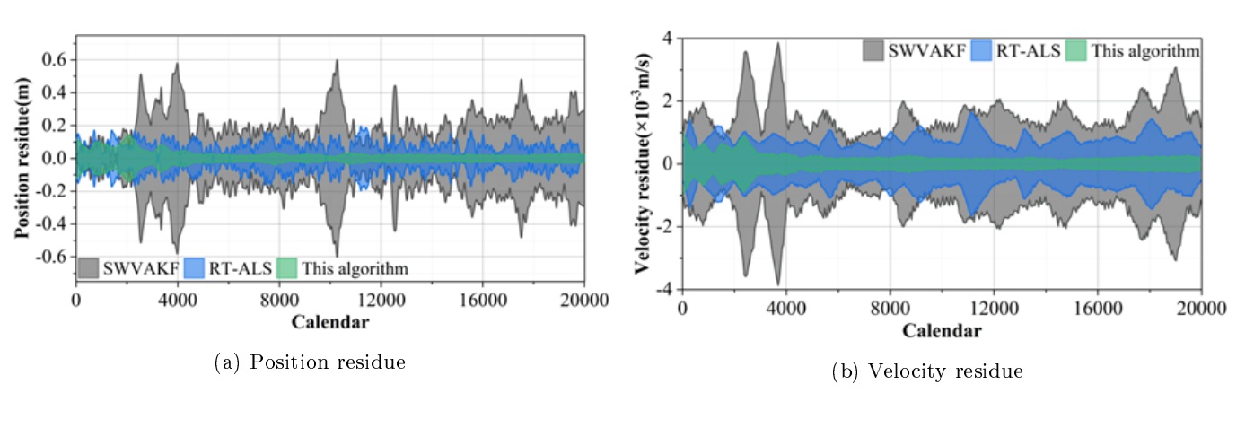
The online filtering results of SWVAKF, RT-ALS and this paper’s adaptive filtering optimization algorithm for the coupling of plateau vortex and atmospheric circulation are shown in Figure 3, where 3a and 3b represent the results of position residuals and velocity residuals of the model’s online filtering, respectively. It can be seen that the position residuals and velocity residuals of the adaptive filtering optimization algorithm proposed in this paper gradually decrease with the increase of the calendar element, and some of the residuals have converged to 0. This is mainly due to the fact that the real-time analysis of the noise covariance has gradually converged to the optimal value, thus obtaining the optimal state valuation. The state valuation residuals of both components of the SWVAKF model are larger than those of RT-ALS, mainly because of the lower analysis accuracy of the SWVAKF adaptive filtering model, and the state valuation residuals of the SWVAKF model become the largest around 4000 and 11000 calendar elements, mainly because the analysis results of the process noise parameter q deviate more from the reference value.
The SRTAE values of the online filtering results of the three methods are shown in Table 1. The SRTAE of both state components of the optimization algorithm proposed in this paper are lower than those of RT-ALS adaptive filtering and SWVAKF model, which are improved by 64.14% and 66.68% compared with RT-ALS adaptive filtering, and 80.24% and 79.33% compared with SWVAKF, respectively. It can be concluded that the state analysis accuracy of the adaptive filtering algorithm optimized based on the LMS criterion gradually improves with calendar elements and is significantly better than the RT-ALS adaptive filtering and SWVAKF model. Overall, the RT-ALS model is affected by the simultaneous inaccuracy of the process noise covariance and the observation noise covariance, and the processing accuracy of the analysis of the plateau eddy coupled with the atmospheric circulation data is limited, while the SWVAKF is limited by the specific matrix structure form of the process noise, and the results of the analysis of the process noise covariance show a large deviation. The two methods not only fail to play the role of noise reduction for the analysis of the coupled data of plateau vortex and atmospheric circulation, but also destroy the beneficial signals contained in the data. The algorithm in this paper, as a real-time adaptive filtering analysis method, is significantly better than the comparative model in terms of both the data analysis processing results and the filtering results. Therefore, the model in this paper is more suitable for the spatial and temporal characterization of the coupling effect of plateau eddies and atmospheric circulation.
| Model | Position component (m) | Velocity component (m/s) |
|---|---|---|
| SWVAKF | 8.214\(\times 10^{-2}\) | 5.623\(\times 10^{-4}\) |
| RT-ALS | 4.526\(\times 10^{-2}\) | 3.487\(\times 10^{-4}\) |
| This model | 1.623\(\times 10^{-2}\) | 1.162\(\times 10^{-4}\) |
Reasonably defining plateau vortices and tracking their movement paths are prerequisites for conducting this study. Currently, there are three main types of algorithms for determining plateau vortices; the first type is based on physical characteristics and defines vortices by setting a threshold value for a particular parameter. The second category is based on the geometrical features of the flow field to determine the vortex by the shape or curvature of the instantaneous flow line; and the third category is the hybrid method, which is a combination of the first two methods. A new method of plateau vortex detection is proposed, which uses high-resolution satellite remote sensing of plateau temperature data to obtain the thermogenic velocity field, identifies the plateau vortex center by analyzing the geometrical features of the thermogenic velocity field, determines the vortex center location, size, polarity, and intensity, and traces its path. Since it completely depends on the geometric features of the flow field, it belongs to the second category of algorithms.
The CFSR data from the National Centers for Environmental Prediction (NCEP) is a new kind of high-resolution reanalysis data of coupled atmospheric circulation with a horizontal resolution of 0.5\(\mathrm{{}^\circ}\)\(\mathrm{\times}\)0.5\(\mathrm{{}^\circ}\), a vertical stratification of 37 layers, and a length of the atmospheric circulation data data data from January 1980 to January 2020, which can be used to find out some fine features in the atmospheric circulation at a much smaller scale. In this paper, the 6-hour-by-6-hour CFSR data are selected, and the selected atmospheric circulation elements include boundary layer height, latitudinal wind speed, meridional wind speed, vertical velocity, friction velocity, and so on.
The data used in this paper include the location of the plateau vortex center, vortex size, vortex polarity, vortex strength, and atmospheric circulation latitudinal wind speed, and the study period is 2000-2020. It should be noted that this paper focuses on the spatial and temporal characteristics of the coupling effect of the plateau vortex and the general circulation in March, because the interannual variability of the vortex on the Tibetan Plateau in March is the largest relative to other months, and previous studies have also focused on the impact of the changes of the plateau vortex on the general circulation in March. For the mechanism analysis, two diagnostic quantities, namely, the intensity of the Tibetan Plateau vortex activity and its induced potential height between the upper troposphere and lower troposphere of the atmospheric circulation, are used in this paper. The data are analyzed using the proposed adaptive filtering optimization algorithm, and the eddy intensity forcing used in the simulation is derived from the eddy intensity forcing output from the Coupled Model Intercomparison Program 5 (CMIP5) model, which is a latitudinally uniform eddy intensity forcing, and the simulation time period is from 2000 to 2020, with a total of 21 years. The results of the simulation and analysis of the spatial and temporal characteristics of the coupled effects of vortex strength and atmospheric circulation on the Tibetan Plateau are shown in Figure 4, with 4a-4c representing the results for the western, central and eastern regions of the Tibetan Plateau, respectively.
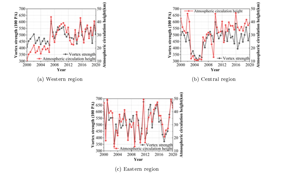
It can be seen that there is a close coupling effect between the vortex intensity and the atmospheric circulation in different spatial and temporal regions of the Tibetan Plateau. Comparatively speaking, the coupling effect between the intensity of the Tibetan plateau vortex in the western and eastern regions of the Tibetan Plateau and the atmospheric circulation in the western region is stronger in terms of the upper tropopause potential height and the lower tropopause potential height, and the average intensity of the Tibetan plateau vortex in the western region reached 603.89 hPa in 2007, and the atmospheric circulation potential height increased to 43.76 km. The intensity of the Tibetan plateau vortex in the eastern region reached 43.76 km in 2001, 2011, and 2019. In 2001, 2011 and 2019, the average strength of the Tibetan Plateau vortex in the western region is 688.21 hPa, 686.00 hPa and 680.93 hPa, respectively, and the height of the atmospheric circulation potential in the simultaneous spatial period of the same year reaches a peak of 49.31 km, 49.38 km and 49.31 km, respectively. The above results show that there is a strong coupling between the vortex strength and the atmospheric circulation over the Tibetan Plateau in different time zones, and that the changes in vortex strength can affect the changes in the potential heights of the upper and lower troposphere of the atmospheric circulation. This coupling implies that the changes of vortex strength on the Tibetan Plateau may affect the atmospheric circulation anomalies.
In this paper, the structure of the adaptive filtering algorithm is optimized using the LMS criterion to improve the performance of the adaptive filtering algorithm in the analysis of plateau eddy and atmospheric circulation data. Through testing experiments to verify the performance of the adaptive algorithm, it is found that the noise parameter and observation noise covariance of the adaptive filter optimization algorithm proposed in this paper are smooth with the increase of calendar elements, and the analysis results are closer to the reference value. The position residuals and velocity residuals of the algorithm gradually decrease with the increase of calendar elements, and some of the residuals tend to zero, which indicates that the effectiveness of the algorithm in the analysis of plateau eddy and atmospheric circulation data has been verified. The analysis of vortex and general circulation data on the Tibetan Plateau during the period of 2000-2020 reveals that there is a close coupling between the strength of the vortex and the general circulation in different spatial and temporal regions of the Tibetan Plateau. In the western part of the Tibetan Plateau, the mean plateau vortex intensity reached 603.89 hPa in 2007, and the atmospheric circulation potential height increased to 43.76 kilometers. The work accomplished in this study verifies the coupling effect between the atmospheric circulation and the plateau vortex, and lays a foundation for the further comprehensive utilization of the anomalous signals of the plateau vortex in different spatial and temporal regions of the Tibetan Plateau to predict the atmospheric circulation characteristics.