
With the increasing frequency of international trade, the economic links between countries are getting closer and closer, and the international competition has become more intense. The real exchange rate reflects the relative high and low price level of the two countries, reflecting the competitiveness of different countries’ commodities in the international market, and its rise and fall will have an important impact on a country’s foreign trade and international economic and trade activities [9,13]. From the end of the 20th century to the beginning of the 21st century, China implemented the strategy of export-led economic development, realizing sustained and high-speed growth of the economy, and the sharp growth of the export and trade surpluses, and accumulating a large amount of foreign exchange reserves, and at the same time, there was a continuous devaluation of China’s real exchange rate. At the same time, China’s real exchange rate experienced continuous depreciation. The Bassa effect suggests that developing countries in the process of high economic growth will be accompanied by real exchange rate appreciation, and the phenomenon of China’s real exchange rate changes deviating from the rapid economic development has aroused strong interest in the academic community [10,14,26]. This may be closely related to the demographic dividend that exists in China, as China has not reached the Lewis inflection point, the demographic dividend has been released in the development of urbanization, and the low labor cost has eased the inflationary pressure and suppressed the appreciation of the real exchange rate [4,6,8].
However, the demographic dividend is not sustainable in the long run. Ageing is both an inevitable result of economic and social development and is also bound to have a greater impact on the economy and society. The aging process will inevitably have a negative impact on a country’s labor force participation rate, technological progress, capital accumulation and economic growth, but also on international capital flows, exchange rates to a certain extent [15,17,19]. From the aspect of international capital flows, population aging will lead to a decline in the proportion of the working population, the relative surplus of capital, reducing the relative return on capital, which will lead to the flow of international capital from the countries with serious aging to the countries with relatively less serious aging [1,12,24,5]. In addition, countries with severe aging have negative current account balances, thus leading to international capital flows from countries with relatively less severe aging to countries with severe aging [16,11,28,23]. In terms of the exchange rate, both international capital outflows and inflows act on the exchange rate, with international capital inflows leading to exchange rate appreciation and international capital outflows leading to exchange rate depreciation [3, 21,7]. With the gradual internationalization of the RMB and the gradual opening of the capital account, the volatility of the RMB exchange rate is also expanding, so it is necessary to study in depth the relationship between population aging and the real effective exchange rate and the impact mechanism [20,2].
This paper points out that the real exchange rate mainly includes the internal real exchange rate and the external real exchange rate, and uses the formula derivation method to show the relationship between the internal real exchange rate and the external real exchange rate. The relationship between population aging and real exchange rate is analyzed from the perspective of demand structure mechanism and current account mechanism. The “Balassa-Samuelson effect” is mentioned, and the transmission mechanism of population aging on the real exchange rate is decomposed through demand changes. Analyze the relationship between population aging, investment rate and current account balance, and establish a trade balance model based on population aging. Interpret the sample data and analyze the impact of population aging on the real exchange rate, the size of the trade surplus and the current account balance, respectively.
The real exchange rate usually consists of two types: the internal real exchange rate and the external real exchange rate.
The internal real exchange rate can be expressed as \(INRER={P_{N} \mathord{\left/ {\vphantom {P_{N} P_{T} }} \right. } P_{T} }\), where \(P_{T}\) represents the domestic price level of the country’s tradable goods and \(P_{N}\) represents the domestic price level of the country’s non-tradable goods. It is essentially the relative prices of non-tradable and tradable goods within a country.
The external real exchange rate can be expressed as \(EXRER={\left(E\times P_{f} \right)\mathord{\left/ {\vphantom {\left(E\times P_{f} \right) P_{d} }} \right. } P_{d} }\), where \(E\) is the nominal exchange rate of the national currency (direct markup method), \(P_{f}\) is the foreign price level, and \(P_{d}\) is the national price level. In theory, the rise in the price of non-tradable goods relative to the price of tradable goods is usually defined as an appreciation of the internal real exchange rate. And the rise in the price of domestic products relative to foreign products is defined as external real exchange rate appreciation.
The relationship between the internal real exchange rate and the external real exchange rate will be demonstrated by the derivation of the formula below. Assuming that the overall price level of a country is equal to the weighted average of the price level of the country’s domestically traded goods and the price level of non-tradable goods, then the overall foreign and domestic price levels can be expressed as: \[\label{GrindEQ__1_} P_{f} =P_{fT}^{\alpha } \times P_{fN}^{1-\alpha } ,\tag{1}\] \[\label{GrindEQ__2_} P_{d} =P_{dT}^{\beta } \times P_{dN}^{1-\beta } ,\tag{2}\] where \(P_{fT}\) and \(P_{fN}\) are the price levels of foreign tradable and non-tradable goods, respectively. \(P_{dT}\) and \(P_{dN}\) are the price levels of domestic tradable and non-tradable goods, respectively. \(\alpha\) is the weight of the price of foreign tradable goods in the overall price level. \(\beta\) is the weight of the price of domestic tradable goods in the overall price level. The external real exchange rate expression is: \[\label{GrindEQ__3_} EXRER = \frac{E \times P_f}{P_d} = E \frac{P_{dT}^{\alpha} P_{dN}^{1-\alpha}}{P_{dT}^{\beta} P_{dN}^{1-\beta}} = \frac{E \times P_f}{P_{dt}} \times \frac{\left( \frac{P_{dT}}{P_{dN}} \right)^{1-\beta}}{\left( \frac{P_{T}}{P_{N}} \right)^{1-\alpha}}.\tag{3}\]
It is evident that \(\frac{E \times P_{fr}}{P_{dT}}\) represents the external real exchange rate, measured using the price of traded goods, and is denoted as \(EXRER_{T}\). Similarly, the ratio \(\frac{P_{dT}}{P_{dN}}\) corresponds to the internal real exchange rate of the domestic country, denoted as \(INRER_{d}\), while \(\frac{P_{fr}}{P_{fN}}\) represents the **internal real exchange rate** of the foreign country, denoted as \(INRER_{f}\).
Thus, the expression for the external real exchange rate can be rewritten as:
\[\label{GrindEQ__4_} EXRER = EXRER_{T} \times \frac{INRER_{d}^{1-\beta}}{INRER_{f}^{1-\alpha}}.\tag{4}\]
Further rewriting Eq. (4) in the form of rate of change gives: \[\label{GrindEQ__5_} \Delta EXRER=\Delta EXRER_{T} +\left(1-\beta \right)\Delta INRER_{d} -\left(1-\alpha \right)\Delta INRER_{f},\tag{5}\] where, \(\Delta\) represents the form of rate of change. Under the assumption that “the law of prices of internationally traded goods is valid”, \(\Delta EXRER_{r}\) is zero, the Eq. (5) can be simplified to: \[\label{GrindEQ__6_} \Delta EXRER=\left(1-\beta \right)\Delta INRER_{d} -\left(1-\alpha \right)\Delta INRER_{f} .\tag{6}\]
It can be seen that rising prices of non-tradable goods are key to the appreciation of a country’s real exchange rate.
In terms of demand, the juvenile and elderly populations are more inclined to consume non-tradable goods than the working-age population, for example, the juvenile population needs education and the elderly population tends to need medical and nursing care. A rise in the share of teenagers and the elderly implies a higher demand for domestic non-tradable goods, which will increase the price of non-tradable goods, and given the price of tradable goods the general price level will rise, eventually leading to an appreciation of the real exchange rate. As can be seen, a rise in the share of a country’s working-age population negatively affects the real exchange rate through the mechanism of the demand structure, leading to a real appreciation of the country’s currency. While a rise in the proportion of juvenile and elderly population will have a positive impact on the real exchange rate through the demand structure mechanism, leading to a real appreciation of the country’s currency.
The current account mechanism means that changes in the age structure of the population will first affect the current account by affecting savings and investment, and changes in the current account will lead to international capital flows, which will further affect the demand for non-tradable goods in each country, thus affecting the price of non-tradable goods and ultimately leading to changes in the real exchange rate.
Life Cycle Theory (LCH) suggests that rational people smooth their consumption over the course of their lives, increasing their savings when they are young and decreasing them when they are old. The teenage and elderly populations have little to no income but need to consume; these populations consume more than they save and are usually considered negative savers. The working-age population, on the other hand, has a source of income, tends to consume less than it earns, and is considered a positive saver. Thus, if a country’s share of the teenage and elderly population rises, the country’s savings will decrease, which will further lead to a current account deficit. In turn, the current account deficit will lead to capital inflows, and the country’s residents will increase their consumption of non-tradable goods, while the prices of non-tradable goods will rise, which will ultimately lead to an appreciation of the real exchange rate.
This paper argues that even though the elderly population may be motivated to save positively for inheritance reasons, their positive savings will usually be lower than those of the working-age population due to their lower incomes. Therefore, if a rise in the share of the elderly population corresponds to a fall in the share of the working population, the country’s aggregate savings will still decline, leading to a current account deficit, capital inflows, and ultimately real exchange rate appreciation.
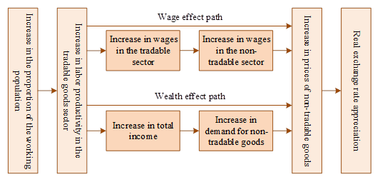
The “Balassa-Samuelson effect” mechanism states that an increase in the proportion of people of working age leads to an increase in the productivity of labor in society as a whole, which causes a general rise in real wages in society. The increase in labor costs leads to an increase in non-tradable prices and an appreciation of the real effective exchange rate. Conversely, an increase in the dependency burden causes the real effective exchange rate to depreciate.
The analysis of the impact mechanism on the supply side of the economy is shown in figure 1, which is framed as follows: in a two-sector economy, the labor productivity in the non-tradable goods output sector of a country (or region) is different from that in the tradable goods sector. It is generally believed that technological improvements will promote productivity gains in the tradable sector, while the role in the non-tradable goods sector is not very obvious, unless the economy meets a large technological innovation or breakthrough. Assuming that a country’s economy is experiencing a period of rapid growth, labor productivity is relatively high in its tradable goods output sector. Higher labor productivity in the tradable goods sector inevitably leads to higher real wages for workers in the tradable goods sector. If the labor force is free to change jobs between the two sectors, then the real wage level in the non-tradable sector will also rise in the same proportion as in the tradable sector, otherwise workers engaged in the production of non-tradable goods will shift to the tradable goods sector. This is despite the fact that the non-tradable sector, without technological innovation, does not have much productivity gain. However, its real wage level will also increase at roughly the same rate as the rest of the sector, and the cost of production determines that the relative price of non-tradable goods will rise.
According to the formula for the internal real exchange rate, the resulting “Balassa” effect suggests that economies experiencing rapid economic growth will also have a marked tendency for the real effective exchange rate to appreciate. The “Balassa-Samuelson” effect bridges the gap between economic growth and the real exchange rate by making use of analytical assumptions such as the free movement of labor across sectors within an economy and differences in labor productivity between the two sectors.
This part uses a comparative static analysis to illustrate the impact of population aging on the real exchange rate through demand movements under market clearing conditions [22,25].
Assume that in the initial equilibrium, country 1 has \(L_{1}\) laborers and \(N_{1}\) seniors. The wage of the labor force in country 1 is \(w_{1}\) times the wage of the labor force in country 2. Country 1 imports the first \(\gamma\) goods, exports the last \(n-k\) goods, and neither imports nor exports the \(\gamma +1\)th through \(k\)th goods. Country 2 has \(L_{2}\) laborers and \(N_{2}\) elderly people, and the wage of country 2’s labor force is unitized to 1. Country 2 exports the first \(\gamma\) goods, imports the next \(n-k\), and neither imports nor exports goods \(r+1\) through \(k\).
The total demand for each commodity in both countries can be obtained by substituting the working population, the elderly population and the wage of the labor force into: \[\label{GrindEQ__7_} Q_{1i}^{D} =\frac{\omega _{1i} \delta _{i} L_{1} }{\left(\rho \left(1+r_{i} \right)+1\right)P'_{1i} } +\frac{\rho \left(1+r_{t-1} \right)\omega _{1t-1} \delta _{i} N_{1} }{\left(\rho \left(1+r_{t-1} \right)+1\right)P'_{1i} },\tag{7}\] \[\label{GrindEQ__8_} Q_{2i}^{p} =\frac{\delta _{i} L_{2} }{\left(\rho \left(1+r_{i} \right)+1\right)P'_{2i} } +\frac{\rho \left(1+r_{t-1} \right)\delta _{i} N_{2} }{\left(\rho \left(1+r_{t-1} \right)+1\right)P'_{2i} } ,\tag{8}\] where, \(Q_{1i}^{p}\) and \(Q_{2i}^{p}\) represent the aggregate demand for commodity \(i\) in countries 1 and 2, respectively. In market equilibrium, all commodities are required to satisfy equal supply and demand. Since country 1 imports the first \(\gamma\) commodities and exports the last \(n-k\) commodities, it neither imports nor exports commodities \(\gamma +1\) through \(k\). Country 2 exports the first \(\gamma\) commodities, imports the second \(n-k\) commodities, and neither imports nor exports commodities \(\gamma +1\) through \(k\). So the demand for the first \(\gamma\) goods in both countries and the demand for goods \(\gamma +1\) through \(k\) in country 2 is supplied by the production of country 2. The demand for the last \(n-k\) goods in both countries and the demand for goods \(\gamma +1\) through \(k\) in country 1 are supplied by production in country 1. The quantity of production of each good in the two countries is: \[\label{GrindEQ__9_} Q_{1i}^{p} =\left\{\begin{array}{l} {0,i\le \gamma }, \\ {Q_{1i}^{D} ,\gamma <i\le k}, \\ {Q_{1i}^{p} +Q_{2i}^{b} ,k<i}, \end{array}\right.\tag{9}\] \[\label{GrindEQ__10_} Q_{2i}^{p} =\left\{\begin{array}{l} {Q_{1i}^{b} +Q_{2i}^{b} ,i\le \gamma }, \\ {Q_{2i}^{p} ,\gamma <i\le k}, \\ {0,k<i}, \end{array}\right.\tag{10}\] where, \(Q_{1i}^{p}\) and \(Q_{2i}^{p}\) denote the total production of commodity \(i\) for country 1 and country 2 respectively. Substituting Eqs. (9) and (10) into Eqs. (7) and (8), respectively, yields the demand for labor for the production of each commodity in each country, and summing them yields the total demand for labor in each country: \[\label{GrindEQ__11_} L_{1}^{D} =\sum\limits_{i=r+1}^{k}\frac{v^{a_{ii} } \left(1-a_{1i} \right)^{a_{1i} } Q_{ii}^{p} }{A_{1i} w_{1}^{a_{1i} } a_{1i}^{a_{1i} } } ,\tag{11}\] \[\label{GrindEQ__12_} L_{2}^{D} =\sum\limits_{i=r+1}^{k}\frac{v^{a_{2i} } \left(1-a_{2i} \right)^{a_{2i} } Q_{2i}^{p} }{A_{2i} w_{2}^{a_{i2} } a_{2i}^{a_{2i} } } ,\tag{12}\] where \(L_{1}^{D}\) and \(L_{2}^{D}\) denote the aggregate demand for labor in country 1 and country 2, respectively. The demand for labor is an increasing function of output and the interest rate, respectively, and a decreasing function of wages. At market equilibrium, the labor market also needs to reach equilibrium between supply and demand, i.e., \[\label{GrindEQ__13_} L_{1} =L_{1}^{D} ,\tag{13}\] \[\label{GrindEQ__14_} L_{2} =L_{2}^{D} .\tag{14}\]
The increase in the number of older persons in country 1 is used as an example to analyze the impact of the increase in the share of older persons in country 1 on the real exchange rate through the demand side. Assume that the number of elderly people in country 1 increases from \(N_{1}\) to \(N'_{1}\).
From Eq. As \(N_{1}\) increases to \(N_{1}\), Country 1’s demand for all goods increases. Since the labor force in both countries is fully employed, supply cannot increase. Under the new market equilibrium condition, the quantity demanded of each individual in both countries for each good must decrease to reach the new market equilibrium.
Since the number of consumers in country 2 remains the same, country 2’s total consumption of each good decreases, i.e., \[\label{GrindEQ__15_} \nabla Q_{2i}^{D} <0 ,\tag{15}\] where, \(\nabla\) indicates the effect of the shock on this variable. Aggregate supply is unchanged because the quantity of labor in the two countries is unchanged. In the new market equilibrium, the aggregate consumption of the two countries remains unchanged, i.e., \[\label{GrindEQ__16_} \nabla \left(Q_{1i}^{D} +Q_{2i}^{D} \right)=0 .\tag{16}\]
From Eqs. (15) and (16), the new market equilibrium shows that the total consumption of all commodities by country 1 increases in the new market equilibrium, i.e., \[\label{GrindEQ__17_} \nabla Q_{1i}^{D} >0 .\tag{17}\]
The change in the price of the commodity in the two countries: \[\label{GrindEQ__18_} \nabla P_{1i} \left\{\begin{array}{ll} {=0,} & {i\le \gamma } ,\\ {>0,} & {\gamma <i\le k{'} }, \\ {>0,} & {k{'} <i} .\end{array}\right.\tag{18}\] \[\label{GrindEQ__19_} \nabla P_{2i} \left\{\begin{array}{ll} {=0,} & {i\le \gamma {'} }, \\ {>0,} & {\gamma {'} <i\le k}, \\ {>0,} & {k<i}. \end{array}\right.\tag{19}\] \[\label{GrindEQ__20_} \nabla P_{1i} \left\{\begin{array}{ll} {=\nabla P_{2i} ,} & {k{'} <i}, \\ {>\nabla P_{2i} ,} & {k{'} >i\ge k} .\end{array}\right.\tag{20}\]
Eqs. (19) and (20) show that in the new market equilibrium, country 1 imports the first \(\gamma {'}\) commodities, exports the last \(n-k\) commodities, and neither imports nor exports commodities from \(\gamma {'} +1\) to \(k\). Since the cost of production increases, country 1 imports more and exports less, i.e. \(\gamma {'} >\gamma\), \(k{'} >k\).
Since the cost of production rises in country 1, the types of goods imported by country 1 increase and the types of goods exported by country 1 decrease, i.e., 5, 6. For country 1, the prices of all non-imported goods rise in the new equilibrium. For country 2, the prices of imported goods also rise in the initial equilibrium.
In the new equilibrium, the price of country 2 increases by the same amount as the price of country 1 for the goods that country 2 still imports. For the goods that Country 2 originally imported and now no longer imports, the increase in the price of Country 2 is less than the increase in the price of Country 1. This is because the price of country 2 for the goods still imported in the new equilibrium and the price of country 1’s goods are determined by country 1’s cost of production, while the original price of the goods no longer imported are determined by country 1’s cost of production. But in the new equilibrium conditions are determined by the cost of production of the two countries, country 2’s cost of production and the original equilibrium cost of imports of the difference is less than the new equilibrium conditions of country 1’s cost of production and the original cost of production difference.
The change in the real exchange rate is: \[\label{GrindEQ__21_} \nabla reer_{1} =\frac{{\sum\limits_{i=1}^{n}\theta _{i} p'_{1i} \mathord{\left/ {\vphantom {\sum\limits_{i=1}^{n}\theta _{i} p'_{1i} \sum\limits_{i=1}^{n}\theta _{i} p_{1i} }} \right. } \sum\limits_{i=1}^{n}\theta _{i} p_{1i} } }{{\sum\limits_{i=1}^{n}\theta _{i} p'_{2i} \mathord{\left/ {\vphantom {\sum\limits_{i=1}^{n}\theta _{i} p'_{2i} \sum\limits_{i=1}^{n}\theta _{i} p_{2i} }} \right. } \sum\limits_{i=1}^{n}\theta _{i} p_{2i} } } .\tag{21}\]
When \(\nabla reer_{1} >1\), it means that the real exchange rate appreciates. A rise in the wage income of the labor force in country 1 causes the real exchange rate to appreciate, i.e., \(\nabla reer_{1} >1\). Thus, population aging causes the real exchange rate to appreciate through the demand side.
Assuming that there is no depreciation, all of a country’s capital accumulation in period t + 1 comes from investment in period t. Capital and factors are freely mobile and the economy is not large enough to affect the level of world interest rates. The level of interest rates in the country depends on the level of interest rates in the international capital market \(R^{W}\), and factor price changes caused by aging in the country have little or no effect on \(R^{W}\). Then the level of interest rates in the country is basically exogenous, and the rise in the savings rate and the increase in the supply of capital caused by aging will not bring about a fall in the level of interest rates, thus effectively stimulating investment. In both the short and the long run, the impact of ageing on investment is mainly reflected in a decline in the level of capital accumulation caused by a fall in the fertility rate, and thus in the gross national investment rate.
The “double-gap model” links financial flows due to the savings-investment gap in an open economy to the current account, i.e., under the condition that government tax revenues are balanced: \[\label{GrindEQ__22_} M-X=I-S^{1} .\tag{22}\]
Divide each side by GDP to get: \[\label{GrindEQ__23_} Cab_{t} =SR_{t} -IR_{t} ,\tag{23}\] where \(Cab_{t}\) is the ratio of current net exports to GDP, which is used to measure the size of the current account balance. The effect of population aging on the current account balance is realized through the separate effects on the savings rate and the investment rate and the contrasting relationship between the two.
Combining the results of the discussion of the savings rate and investment rate, population aging has a positive push on the current account balance in the short run under the assumption of a small country economy, as longer individual life expectancy drives up the level of individual savings and down the level of investment, and domestic capital outflows and trade balances are subjected to upward pressure under the assumption of free capital flows.
Based on the above analysis, the basic proposition of this study is put forward that population aging will have a positive impact on the size of a country’s current account surplus in the short run by affecting the saving and investment rates.
As mentioned earlier, a country’s net exports are equal to the difference between this country’s output and its domestic absorption, and when all variables are effectively laborized in units, the trade balance is: \[\label{GrindEQ__24_} nx_{t} =y_{t} -\left(c_{t} +i_{t} +g_{t} \right) .\tag{24}\]
Substituting Eq. (24) gives: \[ nx_{t} =y_{t} -\left(c_{t} +(x+n+\delta )k_{t} +gy_{t} \right) .\tag{25}\]
Among them: \[ y_{t} =k_{t}^{1-\alpha } ,\tag{26}\]\[ R_{t} =(1-\alpha )k_{t}^{-\alpha } +(1-\delta ) ,\tag{27}\]\[ \label{GrindEQ__28_} c_{t} =\pi _{t} \left\{\left[1+\left(\varepsilon _{t} -1\right)\lambda _{t} \right]R_{t} a_{t} +h_{t}^{w} +\varepsilon _{t} s_{t}^{r} \right\} ,\tag{28}\]\[ \label{GrindEQ__29_} \pi _{t} =1-\beta ^{\frac{1}{1-\rho } } (\Omega R)^{\frac{\rho }{1-\rho } } ,\tag{29}\]\[ \label{GrindEQ__30_} s_{t}^{r} =\theta \tau _{t} y_{t} ,\tag{30}\]\[ \label{GrindEQ__31_} \lambda _{t}^{w} =\frac{\left(1-\tau _{t} \right)\alpha y_{t} }{(1+x+n)(1+n-\gamma )\psi } (1+x+n)-\gamma \omega \left(\beta R_{t} \right)^{\frac{1}{1-\rho } } ,\tag{31}\]\[ \label{GrindEQ__33_} \Omega _{t+1} =\omega +\left(1-\omega _{t} \right)\varepsilon ^{-\frac{1-\rho }{\rho } } . \tag{32}\]
If we look at bilateral trade between the two countries, a surplus in one country necessarily makes a deficit in the other, and the net exports of the two countries are equal in amount and opposite in direction, so by introducing a trading partner country, the balance of trade equation becomes: \[\label{GrindEQ__34_} nx_{t} =0.5\left(y_{t} -y_{t}^{*} \right)-0.5\left[\left(c_{t} -c_{t}^{*} \right)+\left(i_{t} -i_{t}^{*} \right)+\left(g_{t} -g_{t}^{*} \right)\right] ,\tag{33}\] where * denotes foreign countries.
If the differences between the two countries in other respects are not taken into account, but only the further change in net exports due to differences in the age structure of the population in terms of total social property and total marginal propensity to consume of the society, i.e., \[\label{GrindEQ__35_} \begin{array}{l} {nx_{t} =-0.5\pi _{t} } {\left[R\left(a_{t} -a_{t}^{*} \right)+\left(\varepsilon _{t} -1\right)R\left(\lambda _{t} a_{t} -\lambda _{t}^{*} a_{t}^{*} \right)+\left(h_{t}^{*} -h_{t}^{w^{*} } \right)+\varepsilon _{t} \left(s_{t}^{r} -s_{t}^{r^{*} } \right)\right]}. \end{array}\tag{34}\]
Eq. (35) can be further simplified if both countries have the same effective labor capital per unit, social wealth, after-tax labor income for workers, and transfer income (pensions) from the government for retirees, and if the modeling assumption that the marginal propensity to consume of retirees is greater than that of workers, i.e., \(\left(\varepsilon _{t} -1\right)>0\), is satisfied: \[\label{GrindEQ__36_} nx_{t} =-0.5\pi \pi _{t} \left(\varepsilon _{t} -1\right)Ra_{t} \left(\lambda _{t} -\lambda _{t}^{*} \right) .\tag{35}\]
Substitution gives: \[\label{GrindEQ__37_} nx_{t} =-0.5\pi _{t} \left(\varepsilon _{t} -1\right)Ra_{t} \frac{(1+x+n)(1+n-\gamma )}{(1+x+n)-\gamma \omega \left(\beta R_{t} \right)^{\frac{1}{1-\rho } } } \left(\psi _{t} -\psi _{t}^{*} \right) .\tag{36}\]
It is clear that \(\left(\psi _{t} -\psi _{t}^{*} \right)>0\) when the aging level of the country is higher (or faster) than that of the foreign country, and \(\left(\psi _{t} -\psi _{t}^{*} \right)\) is negatively related to \(nx_{t}\). Therefore, when the aging level of the country is higher or faster compared to that of the foreign country, then the balance of trade of the country will deteriorate. This deterioration in the balance of trade is due to the fact that the increase in the degree of aging causes a change in the distribution of the total wealth of the society among the different age groups. It is also caused by differences in the marginal propensity to consume of individuals in different age groups.
Similarly, if the two countries in the unit of effective labor capital, social wealth, age structure are the same premise, we have: \[\label{GrindEQ__38_} \begin{cases} {nx_{t} =-0.5\pi _{t} \left(h_{t}^{*} -h_{t}^{w^{*} } \right)} ,\\ {nx_{t} =-0.5\pi _{t} \left[-\alpha y_{t} \left(\tau _{t} -\tau _{t}^{*} \right)+\varepsilon _{t} y_{t} \left(\theta _{t} \tau _{t} -\theta _{t}^{*} \tau _{t}^{*} \right)\right]}. \end{cases}\tag{37}\]
Substitution gives: \[\label{GrindEQ__39_} nx_{t} =0.5\pi _{t} \alpha y_{t} \left(\tau _{t} -\tau _{t}^{*} \right) .\tag{38}\]
It is clear from the equation that the tax rate of the country relative to foreign countries \(\left(\tau _{t} -\tau _{t}^{*} \right)\) is positively related to the trade balance of the country \(nx_{t}\), which indicates that when the country raises the tax rate relative to foreign countries, it will improve the trade balance of the country, which is due to the increase in the tax rate that reduces the disposable income of the individual and thus suppresses the consumption of the individual.
If both countries have the same effective labor capital per unit, social wealth, age structure and after-tax labor income of workers, we have: \[\label{GrindEQ__40_} nx_{t} =-0.5\pi _{t} \varepsilon _{t} \left(s_{t}^{r} -s_{t}^{r^{*} } \right) .\tag{39}\]
Substitution gives: \[\label{GrindEQ__41_} nx_{t} =-0.5\pi _{t} \varepsilon _{t} \tau _{t} y_{t} \left(\theta _{t} -\theta _{t}^{*} \right) .\tag{40}\] When the transfer expenditure of the home government on the elderly population increases relative to foreign countries, i.e., \(\left(\theta _{t} -\theta _{t}^{*} \right)>0\), the home country’s balance of trade deteriorates, a deterioration that is caused by an increase in the income of the elderly population leading to an increase in the consumption demand of the society as a whole.
After discussing the three scenarios separately, we will further analyze the scenario where the three scenarios coexist, because in practice, as the aging process of a country continues, it will cause the government of that country to pay more attention to the problem of aging. And further increase the investment in the elderly population, and the increase in investment may further cause an increase in tax revenue. Such as some of the Nordic countries with a high degree of aging show the characteristics of high welfare and high taxes.
It can be seen that as a country ages more, an increase in the dependency ratio worsens the balance of trade. At the same time, an increase in transfer income to the aging population likewise worsens the balance of trade. However, there may be uncertainty about the impact of higher tax rates on the balance of trade. This is because higher tax rates can discourage consumption, which can improve the balance of trade. However, higher tax rates can lead to more transfer income for the elderly population. This, in turn, stimulates consumption through increased income and can worsen the trade balance.
In order to empirically test the impact of population aging on the internal real exchange rate, the benchmark panel model constructed in this paper is as follows: \[\label{GrindEQ__42_} irer_{it} =c_{0} +c_{1} oldrate_{it} +Z'_{it} c_{2} +\mu _{i} +\varepsilon _{it} ,\tag{41}\] where \(irer_{it}\) denotes the internal real exchange rate, \(oldrate\) denotes the degree of population aging, and \(\mu _{i}\) is the individual effect, \(\varepsilon _{it}\) is the disturbance term, and \(Z'_{it}\) is the matrix of control variables.
In order to answer the question of whether deeper aging causes an increase in the internal real exchange rate, the combined impact effect is estimated using a benchmark regression. Meanwhile, in order to further answer the question of how an increase in the share of the aging population affects the internal real exchange rate through two transmission paths: the Bassa effect and the demand structure effect. The mediation effect method is used for empirical testing, and the relevant model is: \[\label{GrindEQ__43_} M_{it} =a_{0} +a_{1} oldrate_{it} +Z'_{it} a_{2} +\mu '_{i} +\varepsilon '_{it} ,\tag{42}\] \[\label{GrindEQ__44_} irer_{it} =b_{0} +b_{1} oldrate_{it} +Z'_{it} b_{2} +b_{3} M_{it} +\mu ''_{i} +\varepsilon ''_{it} .\tag{43}\]
In Eqs. (42) and (43), \(M_{it}\) is the mediating variable, which is the proxy variable for the Bassa effect and the demand structure effect. According to the test steps of the stepwise regression method of the mediation effect test, the first regression of Eq. (44) is conducted to test whether the estimated parameter cl of population aging on the internal real exchange rate is significantly positive, and if it is significantly positive, it means that the increase in aging rate leads to the increase in the value of the internal real exchange rate. Secondly, the regression of Eq. (42) is conducted to test whether the coefficient a1 of the aging rate on the mediating variable is significant. Finally, Eq. (43) is tested to determine the significance of b1 and b3. If b3 is significant, it means that the mediating effect is established. If b1 is significant, it is a partial mediation effect, and vice versa, it is a full mediation effect.
Based on the inter-provincial panel data of 29 provinces and cities from 2001 to 2023, this paper constructs a fixed-effects model to test the impact of population aging on the real exchange rate. It also introduces two intermediary variables, relative labor productivity and demand structure, to empirically test the reasonableness of the existence of the two transmission mechanisms.
The internal real exchange rate is decomposed from the real exchange rate, which is defined as the ratio of the price of the products of the non-tradable and tradable sectors in a country measured in the currency of that country, and it is necessary to clarify the division of the non-tradable sectors and tradable sectors before measuring this index.
In this paper, the secondary industry is divided into tradable sectors and the tertiary industry is divided into non-tradable sectors. Firstly, according to the value added of the secondary and tertiary industries at constant price in 2001 as well as the value added index in each province, the value added of the secondary and tertiary industries at constant price in each year is calculated in each province. Secondly, the price index of the secondary and tertiary industries in each province is obtained by dividing the value added at current price by the value added at constant price. Finally, the ratio obtained by dividing the price index of the tertiary industry by the price index of the secondary industry is the internal real exchange rate of each province.
In the robustness test of this paper, the old age dependency ratio is regressed as a variable replacing the proportion of population aged 65 and above. Both variables are logarithmized.
In this paper, GDP per capita, local government expenditure, foreign direct investment, land finance, rural labor force transfer, and openness are selected as control variables. The description of the control variables is as follows:
GDP per capita (rgdp): GDP per capita is a measure of the income effect, a rise in GDP per capita indicates a rise in the income of the population and an increase in the consumption of non-tradable goods thereby increasing the internal real exchange rate. This effect is controlled for here using GDP per capita from the statistical yearbook, and the results are logarithmized.
Local government expenditures (gov): the share of general budget expenditures of each provincial government in regional GDP is used as a proxy variable for government expenditures, and the results are logarithmized.
Foreign direct investment (fdi): use the share of foreign direct investment in GNP of each province multiplied by 100 to express foreign direct investment.
Land finance (lfi): in order to control for the impact of land finance, this paper uses the share of state-owned land use right transfer revenue in the budgeted local fiscal revenue of each province as a proxy variable for land finance.
Rural labor force transfer (tra): using the gap between the per capita annual income of urban and rural residents as a proportion of the per capita annual income of rural residents as a proxy variable for rural labor force transfer for empirical regression.
Openness (open): use the total import and export of each province as a proportion of the province’s GDP to portray this indicator.
Relative labor productivity (pro): Using the GDP of the secondary and tertiary industries and the corresponding employment in each province in the statistical yearbook, the per capita output of each industry in each province is calculated, and the per capita output of the tertiary industry is divided by the per capita output of the secondary industry to get the relative labor productivity and logarithmic processing.
Demand structure (demstr): The ratio of per capita consumption expenditure of the tertiary industry to that of the secondary industry in each province is used to portray the structure of consumer demand.
Descriptive statistics of the main variables are shown in Table 1.
| Variable | Sample size | Mean | Standard deviation | Minimum value | Maximum value |
|---|---|---|---|---|---|
| Actual effective exchange rate | 1569 | 100.96 | 15.37 | 45.08 | 293.44 |
| Elderly dependency ratio | 1569 | 8.25 | 6.78 | 1.97 | 30.56 |
| International capital flow | 1569 | -3.02 | 13.43 | -412.31 | 152.83 |
| Economic growth | 1569 | 2.14 | 4.12 | -21.06 | 19.79 |
| Openness | 1569 | 66.89 | 40.37 | 13.75 | 346.01 |
| Domestic money supply | 1569 | 63.05 | 39.86 | 7.21 | 264.12 |
| Inflation level | 1569 | 91.43 | 35.71 | 4.03 | 389.47 |
The data sources are the same as above, and the explanatory variables, explanatory variables and control variables selected in the model are specified below.
The explanatory variable is the trade balance, and the net export value of the location of the business unit is used as the proxy variable for the trade balance, which is denoted as NE. The explanatory variables are selected as the old-age population dependency ratio (OLD), the natural population growth rate (NPG), and population mobility (MI). The old-age population dependency ratio is the proportion of the population aged 65 and above to the working population aged 15-64. The degree of aging of the elderly population is negatively correlated with net exports. The natural population growth rate (NPG) is the ratio of the natural increase in the population (births – deaths) over a certain period of time to the average total population over the same period of time, and the natural population growth rate is negatively correlated with net trade exports. Population mobility (MI), i.e., the movement of people between regions within a certain period of time. This paper measures population mobility by subtracting the resident population from the household population and dividing by the household population, and population mobility is negatively correlated with net trade exports.
The control variables are foreign direct investment (FDI), local public financial expenditure (GOV), social fixed asset investment (INV), total retail sales of consumer goods (CON) and per capita GDP growth rate (PGDP).
Foreign direct investment (FDI), i.e. investment activities carried out by foreign investors to obtain investment income, operation rights, control rights, FDI can measure the level of the region’s openness to the outside world, and international trade shows a high degree of correlation and development of convergence, the capital export promotes the export trade, and the two show a positive correlation.
Local public finance expenditure (GOV), i.e. the nominal value of local public finance expenditure in each province, measures government expenditure. Local government expenditure has a crowding-out effect on national savings, while pushing up the investment rate, resulting in a narrowing of the savings and investment gap and a decline in net exports, so the coefficient of local fiscal expenditure is negative.
Social investment in fixed assets (INV), is a comprehensive indicator reflecting the scale, speed, proportion and direction of use of investment in fixed assets. According to the net export is equal to savings minus investment, an increase in investment will lead to a decline in net export, so the investment coefficient is negative.
Total retail sales of consumer goods (CON), is a direct indicator of consumer demand. Consumption and net exports have a complementary relationship in both the long and short term, and consumption growth has a positive relationship with net export growth.
The descriptive statistics of the relevant variables are shown in Table 2.
| Variable name | Unit | Symbol | Observed value | Mean value | SD | Min | Max |
|---|---|---|---|---|---|---|---|
| Net export | Billion | NE | 1569 | 9.66 | 59.68 | -310.55 | 273.43 |
| Older people’s oral dependency ratio | % | OLD | 1569 | 13.52 | 3.04 | 7.45 | 23.55 |
| Natural growth rate of population | % | NPG | 1569 | 6.31 | 3.22 | -1.07 | 13.46 |
| Population mobility | % | MI | 1569 | 3.76 | 17.45 | -21.86 | 70.23 |
| Local public expenditure | Billion | GOV | 1569 | 31.46 | 25.78 | 1.25 | 159.46 |
| Total retail sales of consumer goods | Hundredbillion | CON | 1569 | 7.07 | 6.45 | 0.09 | 40.15 |
| The whole club will invest in fixed assets | Hundredbillion | INV | 1569 | 12.51 | 11.74 | 0.18 | 56.73 |
| Foreign direct investment | Billion | FDI | 1569 | 6.98 | 8.62 | 0.06 | 36.92 |
| Total retail sales of consumer goods | Hundredbillion | CON | 1569 | 7.05 | 7.69 | 0.12 | 40.15 |
The empirical results of the regression model (explanatory variable: real effective exchange rate) are shown in Table 3. Column 2 shows the empirical results of the regression based on data for the full sample of countries. Column 3 shows the empirical results of the regression based on data for the super-aging countries. Column 4 shows the empirical results based on regressions with data from deeply aging countries. Column 5 shows empirical results based on regressions with data from mildly aging countries, and column 6 shows empirical results based on regressions with data from non-aging countries.
The results show that the old-age dependency ratio is an important influence on the real effective exchange rate. From the full sample of countries, the coefficient of the old-age dependency ratio in column 2 is 1.5263 and significant at the 1% statistical level, indicating that a rise in the old-age dependency ratio will lead to a rise in the real effective exchange rate. That is to say, both statistical significance and economic significance, the old-age dependency ratio will have a significant uplifting effect on the real effective exchange rate. That is, aging will lead to real effective exchange rate appreciation.
From the empirical results of the sample country subgroups, the relationship between the impact of the old-age dependency ratio on the real effective exchange rate is significantly heterogeneous. The coefficients of the old-age dependency ratio of super-aging countries and mildly aging countries are all negative and significant at the 1% statistical level, indicating that a rise in the old-age dependency ratio will drive down the real effective exchange rate. The coefficients of the old-age dependency ratios of deeply aging countries and non-aging countries are positive and significant at the 10% statistical level, indicating that a rise in the old-age dependency ratio will lead to a rise in the real effective exchange rate. In conclusion, countries in the stage of super-aging and mild aging, aging will lead to the depreciation of the real effective exchange rate. In the stage of deeply ageing and non-ageing countries, ageing leads to real effective exchange rate appreciation.
| Interpretation variable | All sample countries | Ultra aging country | Country of deep aging | A mild aging country | The unaged country |
|---|---|---|---|---|---|
| Elderly dependency ratio | 1.5263 (0.006) | -2.3965 (0.001) | 4.2798 (0.000) | -3.2604 (0.015) | 4.3587 (0.072) |
| Economic growth | -0.2047 (0.223) | 0.6352 (0.153) | -0.0752 (0.804) | -0.0268 (0.717) | -0.4213 (0.167) |
| Openness | -0.2586 (0.000) | 0.2368 (0.003) | -0.1675 (0.063) | -0.3684 (0.000) | -0.2255 (0.003) |
| Domestic money supply | 0.0725(0.136) | -0.0596(0.008) | -0.1042(0.039) | 0.1024(0.065) | 0.1423(0.204) |
| Inflation level | -0.0869(0.000) | 0.7961(0.000) | -0.1023(0.711) | 0.1382(0.003) | -0.1639(0.000) |
| Constant term | 125.003(0.000) | 0.7968(0.000) | -0.1207(0.823) | 0.1346(0.003) | -0.1785(0.000) |
| Observed value | 1569 | 135 | 365 | 489 | 580 |
| Hausman Test | Fixed effect model | Fixed effect model | Fixed effect model | Fixed effect model | Fixed effect model |
| F statistic | 15.23(0.001) | 75.39(0.001) | 5.06(0.001) | 22.57(0.000) | 14.36(0.000) |
Setting up the estimated, we have: \[\label{GrindEQ__45_} cl_{it} =\beta _{0} +\beta _{1}^{*} oldrate_{it} +\beta _{2} X_{it} +\varepsilon _{it} ,\tag{44}\] where \(cl\) is the international capital flow variable, \(ageo\) is the old age dependency ratio, \(X\) is the control variable and \(\varepsilon\) is the error term.
The empirical results of the regression model (explanatory variable: international capital flows) are shown in Table 4. From the full sample of countries, the coefficient of the old age dependency ratio in column 2 is 0.3291 and is not significant at the 10% statistical level, indicating that the increase in the old age dependency ratio does not have an impact on net international capital inflows.
| Interpretation variable | All sample countries | Ultra aging country | Country of deep aging | A mild aging country | The unaged country |
|---|---|---|---|---|---|
| Elderly dependency ratio | 0.3291(0.526) | 0.3215(0.102) | -1.0236(0.423) | 1.8224(0.000) | -2.1405(0.047) |
| Economic growth | -0.2136(0.082) | 0.2518(0.072) | -1.0036(0.042) | 0.0362(0.713) | 0.1708(0.142) |
| Openness | -0.0321 (0.0745) | -0.1311(0.008) | 0.1367(0.412) | -0.0252(0.301) | -0.0796(0.005) |
| Domestic money supply | -0.0235(0.721) | -0.0663(0.085) | -0.0082(0.915) | -0.0721(0.018) | 0.0063 (0.0811) |
| Inflation level | -0.0125(0.217) | 0.2635(0.000) | -0.0182(0.906) | -0.0415(0.15) | -0.0241(0.068) |
| Constant term | -0.7251(0.855) | -20.1214(0.001) | 14.2351(0.457) | -10.0213(0.003) | 12.4058(0.007) |
| Observed value | 1569 | 135 | 365 | 489 | 580 |
| Hausman Test | Fixed effect model | Fixed effect model | Fixed effect model | Fixed effect model | Fixed effect model |
| F statistic | 1.56(0.635) | 7.46(0.003) | 1.73(0.362) | 5.21(0.003) | 4.57(0.000) |
That is, aging is not a significant influence on net international capital inflows. The main reason is that population aging may affect international capital flows through two paths, the capital-labor ratio and the current account balance, but the effects of the two paths cancel each other out, resulting in a non-significant effect on net international capital inflows.
The empirical results of the sample country groupings show that the relationship between the impact of the old-age dependency ratio on international capital inflows is significantly heterogeneous.
In mildly aging countries, unaging countries and other countries with low aging, the coefficient of the old-age dependency ratio is significant at the 5% statistical level, indicating that a rise in the old-age dependency ratio significantly affects international capital flows.
In countries with a high degree of ageing, such as the super-ageing countries and the deeply ageing countries, the coefficient on the old-age dependency ratio is not significant at the 10 per cent statistical level, suggesting that an increase in the old-age dependency ratio would not significantly affect international capital flows.
Impact of population ageing on the size of trade surplus: The regression results of the benchmark model are shown in Table 5. Models (1) and (2) use the proportion of the population aged 60 years or older as a proxy variable for population ageing. Models (3) and (4) use the old-age population dependency ratio as a proxy variable for population aging for robustness reasons, accounting for the regression results obtained in the econometric model.
Columns (1) and (3) select economic size (lnGDP), R&D investment (RDR), human capital (EDU), and urbanization level (URBAN) as control variables. Columns (2) and (4) add the growth rate of GDP per capita (GPCG), the level of capital stock per capita (CSPPS), the share of loan balance (LOANR), the local fiscal policy (FIDER), the scale of foreign direct investment (FDIR), and the level of social security expenditures (ESSER) to columns (1) and (3), respectively, to further control for the omitted variables that cause bias in the estimation of the estimation bias of the core variables.
The regression results from columns (1) to (4) show that this suggests that at the provincial level, the development of an aging population at this stage will result in further accumulation of current account surpluses. This result is consistent with the theoretical model.
According to the discussion of the theoretical analysis, population aging realizes the impact on the current account balance by exerting influence on the national saving rate and investment rate respectively. In order to verify the mechanism of the impact of population aging on the current account balance, the mediating variables national saving rate and investment rate are introduced to examine whether the impact mechanism is in line with the theoretical expectations. The mechanism analysis of the impact of population aging on the size of trade surplus is shown in Table 6.
| Explained variable | ||||
|---|---|---|---|---|
| Trade surplus | (1) | (2) | (3) | (4) |
| AGPR | 0.496**(0.367) | 0.499**(0.223) | – | – |
| ODEP | – | – | 0.321*(0.175) | 0.325*(0.174) |
| Constant term | -120.369***(15.673) | -150.336***(16.403) | -112.521***(14.507) | -142.331*** (16.204) |
| Other control variables | yes | yes | yes | yes |
| Year control variable | yes | yes | yes | yes |
| Provincial control variable | yes | yes | yes | yes |
| Observed number | 1569 | 1569 | 1569 | 1569 |
| \(r2\_ p\) | 0.365 | 0.378 | 0.385 | 0.392 |
| \(p\) | 0 | 0 | 0 | 0 |
| Variable name | Saving rate | Investment rate | ||||||
|---|---|---|---|---|---|---|---|---|
| (1) | (2) | (3) | (4) | (5) | (6) | (7) | (8) | |
| AGPR | 1.362***(0.368) | 1.124***(0.279) | – | – | 0.135(0.629) | -0.237(0.768) | – | – |
| ODEP | 0.899***(0.235) | 0.789***(0.195) | 0.053(0.461) | -0.152(0.362) | ||||
| Constant | 32.262***(4.527) | -172.632**(22.504) | 33.526***(3.072) | -153.396**(25.635) | 32.632***(7.504) | 55.362(45.107) | 33.956***(7.024) | 55.236 (45.115) |
| Other control variables | yes | yes | yes | yes | yes | yes | yes | yes |
| Year control variable | yes | yes | yes | yes | yes | yes | yes | yes |
| Provincial control variable | yes | yes | yes | yes | yes | yes | yes | yes |
| Observed value | 1569 | 1569 | 1569 | 1569 | 1569 | 1569 | 1569 | 1569 |
| R-squared | 0.812 | 0.855 | 0.733 | 0.824 | 0.659 | 0.674 | 0.819 | 0.725 |
| r2 | 0.812 | 0.855 | 0.733 | 0.824 | 0.659 | 0.674 | 0.819 | 0.725 |
| N | 1569 | 1569 | 1569 | 1569 | 1569 | 1569 | 1569 | 1569 |
Using the fixed-effects model, the impact of population aging on the national savings rate is examined on the basis of controlling the province effect and the year effect.
Models (1) and (3) are the estimation results without adding other control variables using the proportion of the elderly population and the elderly population dependency ratio, respectively. Models (2) and (4) are the estimation results with the addition of control variables affecting savings and investment, respectively. It can be seen that the population aging indicator significantly affects the national saving rate under different model settings. Models (5)-(8) use a fixed effects model to examine the impact of population aging on the investment rate. It can be seen that the effect of population aging on investment is not significant under different model settings. It shows that population aging does not have a significant impact on the current account balance through investment under the selected sample. Population aging positively affects the trade surplus at the provincial level mainly by affecting the level of savings.
This paper analyzes the correlation between population aging and the real exchange rate, and proposes a model of the impact between population aging and the real exchange rate by integrating the “Balassa-Samuelson effect”. It also decomposes the impact of population aging on the trade balance, and establishes the impact model of population aging and current account balance.
1) The coefficient of the old-age dependency ratio of all samples is 1.5263, and it is significant at 1% statistical level, showing that the old-age dependency ratio is an important factor influencing the real effective exchange rate, and the rise of the old-age dependency ratio will drive the real effective exchange rate to rise. Population aging and international capital flows in the empirical test, reflecting the old age dependency ratio on the international capital inflows of the impact of the relationship has obvious heterogeneity.
2) The regression analysis of the benchmark model of population aging on the size of trade surplus finds that, at the provincial level, the degree of aging does have a positive impact on the trade surplus by increasing the level of residents’ savings, which is consistent with the findings of the theoretical analysis. This indicates that population aging has a positive impact on the trade surplus at the provincial level mainly by affecting the level of savings.