
Enterprises face enormous competitive pressure in the digital era, and in order to adapt to this change, various industries have carried out digital transformation. The supply chain, as the main component of enterprise operation, utilizes advanced technologies such as the Internet of Things, big data analysis, artificial intelligence, etc., in the digital transformation process to monitor, analyze and apply the data of each link in real time, which realizes the intelligent management and optimization of the supply chain [13, 17].
For the majority of manufacturing industries, it is essential for them to increase the importance of supply chain cost control [12]. Supply chain cost management includes the costs that need to be invested in material procurement, the costs that need to be invested in the process of product marketing and promotion, and the costs that need to be invested in the process of production and manufacturing [3, 11]. The existence of supply chain cost management, to a large extent, can promote the extension of internal cost control work, and ultimately develop into a management behavior across multiple departments in the enterprise, which can have a direct impact on the enterprise’s transaction and cooperation object selection [20, 23, 8, 15]. In addition, digital transformation of an enterprise requires it to adjust the way it allocates resources according to the digital technology paradigm [14]. Digitally transformed enterprises are characterized by flexibility and ease of change, and can adapt quickly to reconfigure resources and develop new capabilities [5, 4]. In particular, they establish strong new connections with other stakeholders through digital platforms or networks, expand into new areas, identify new market opportunities and create value through strategic approaches [9, 10, 21].
Tiwari et al. [17] showed that big data analytics is one of the best techniques for supply chain professionals to deal with the massive amount of data generated in end-to-end supply chain management practices by investigating and analyzing the data to provide valuable insights to the industry. Gunasekaran et al. [7] investigated the impact of big data predictive analytics (BDPA) on supply chain (SCP) and organizational performance (OP) and clarified the mediating effect of connectivity and information contributing resources in executive commitment based on a resource-based perspective. Gopal et al. [6] analyzed the impact of big data analytics capabilities on the development of retail supply chains, and found that big data practices can provide retailers who are caught in a dilemma between customer loyalty and cost with importance and dominance assessment based on the optimal decision-making. Zhang et al. [22] proposed a dynamic scheduling method for logistics supply chain based on adaptive ant colony algorithm, constructed a dynamic scheduling model of the supply chain based on the constraints, and introduced the adaptive ant colony algorithm to solve the optimal dynamic scheduling scheme for logistics supply chain. The cost control method of mobile e-commerce under the information of big data, and utilized the intelligent and digital means to analyze the internal and external problems of the supply chain and establish an enterprise supply chain cost control model based on this. Xue et al. [19] used cloud genetic algorithm as the basis and means of quality management and cost control in the long-term operation of logistics service supply chain, and proposed suitable supply chain construction method and cost optimization method, aiming to construct and operate logistics service supply chain in the form of high quality with lower cost.
This paper analyzes the necessity of using big data to optimize supply chain cost control, takes big data technology as the technical support for enterprise cost management, and designs the supply chain cost control procedure based on big data. The intelligent sales forecast is constructed, the CPFR theory is introduced, and the CPFR sales combination forecast model is formed by combining the time series forecast model and the multiple regression model. For the inventory optimization based on supply chain coordination, safety stock design is added to form the supply chain inventory optimization program for product demand forecast. The time series forecasting model and multiple regression forecasting model are validated separately, and the forecasting results of the two are synthesized to obtain the combined forecasting effect. Based on the sales forecast, inventory surplus calculation is carried out and flexible ordering is implemented. The optimization effect of the inventory optimization scheme based on big data sales forecast on supply chain cost control is analyzed in terms of procurement cost and operation cost.
Supply chain in enterprise development occupies an increasingly important position, is the enterprise “the third source of profit”, supply chain is not only the point of enterprise cost generation but also the focus of cost reduction [1,2].
Supply chain cost control not only includes the internal cost of the enterprise, but also includes the cost between the supply chain and other enterprises. The ultimate goal of supply chain cost control is the optimization and reduction of the total cost of the whole supply chain. The application of big data technology in each link of the supply chain can reduce the cost of each link and increase the efficiency of the enterprise, thus improving the comprehensive competitiveness of the company.
For the supply chain to play its due role, it is not only necessary to see whether the whole supply chain can reduce costs for the company, but also to see whether the company’s supply chain is reasonable, i.e., whether the operation efficiency is efficient.
The company’s supply chain management covers all aspects of R&D, procurement, production, sales and logistics. The complex and changing internal and external operating environment requires the company to make operational decisions quickly. The use of big data technology can help the company accurately locate the balance point of various operational decisions from the complicated influencing factors, so as to reach the long-term, dynamic global optimal wisdom decision. The company can utilize big data technology to improve the existing supplier database, so as to facilitate the rapid screening of suitable suppliers to shorten the procurement time, thus improving the procurement efficiency. At the same time in the production can also use big data technology to predict the amount of inventory, etc. to improve production efficiency. It can be seen that the application of big data technology to all aspects of the company’s supply chain, in order to achieve intelligent prediction, intelligent demand, intelligent procurement, etc., to improve the efficiency of the supply chain operation.
With the development of information technology, big data technology provides strong support for enterprise cost management. Based on the reasonable collection of data information generated by various aspects of the business of the enterprise, the cost data information is quantified through professional information processing technology. The company needs to improve the process of big data supply chain cost control, and implement relevant improvement measures according to the standards, so that the supply chain cost control program can be effective. The supply chain cost control program based on big data is shown in Figure 1.
Prior prediction refers to the enterprise before incurring costs, based on the historical cost data of each link of the enterprise supply chain, using big data prediction technology to comprehensively predict and analyze the costs that may be incurred by each link of the enterprise supply chain. From there, it determines the standard cost of each link of the supply chain of the enterprise under normal operation and establishes a standard cost database. As a measure of enterprise supply chain cost overspending or saving standards, so as to realize cost control beforehand.
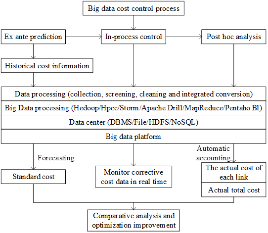
Ex-ante control refers to the enterprise with the help of big data platform, real-time supervision of the cost of each link of the enterprise supply chain and the degree of impact on the total cost of the supply chain, timely detection of problems, real-time supervision and correction of errors. Timely adjustment of solutions according to changes in specific problems. The big data analysis platform shortens the cycle from data extraction to offline analysis and then to report production, eliminating the need to repeat the number of withdrawals, and the marginal cost tends to be close to zero, which significantly reduces the time and labor costs.
Post-facto analysis refers to the fact that after generating costs, the enterprise automatically accounts for the actual costs of each link in the supply chain for a certain period of time with the help of the big data platform, compares the standard costs in the database established in the pre-prediction, analyzes the causes of the discrepancies and pursues the responsibility, reports to the corresponding management and decision-making levels in a timely manner, formulates the solutions, and sums up the experience to optimize and improve the existing measures.
Sales forecasting, as the first part of supply chain management, should be a key concern for enterprises. Reasonable and accurate sales forecasts can help enterprises adjust their short-term development plans and marketing strategies, and rationally deploy their daily management.
Generally speaking, sales forecasting should not only take into account the external market demand, economic environment and other factors, but also consider the enterprise’s own market positioning, product price prediction and promotion strategy and other factors. Therefore, building a sales forecasting system helps to do a good job of strategic planning, adjusting its sales quota, rationally managing cash flow, and then improving the efficiency of resource allocation.
The flow of the intelligent sales forecasting system is shown in Figure 2. Using visual analysis tools, the order analysis situation, inventory data and internal and external factors of offline stores are summarized and analyzed. It also extracts the characteristics of each commodity type and constructs the corresponding sales prediction model. The system finally derives various scenarios of total sales forecast of commodities, single-point sales forecast of different regions, and single product forecast of different types of the same commodity. The above forecasts are then transmitted to the purchasing system for coordination and communication between the purchasing department and suppliers.
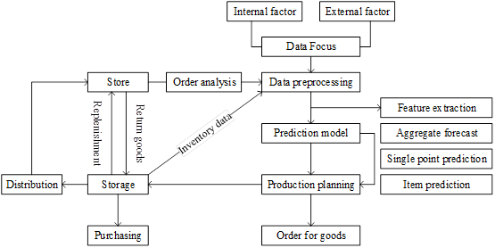
By utilizing big data technology, the Intelligent Sales Forecasting System can build an endless system of indicators based on different merchandise types and scenarios, thus helping management reduce the time it takes to make important business decisions. In addition, from marketers to store managers to purchasing specialists, the forecasting system can provide insightful analytics to members in all segments of the supply chain as a way to help people in all departments make proactive, quick decisions.
CPFR is collaborative supply chain inventory management, i.e., collaborative planning, forecasting and replenishment, which is a collaborative supply chain inventory management technique and an important strategy of collaborative supply chain management.
CPFR not only requires relevant units upstream and downstream of the supply chain to implement joint forecasting and replenishment, but also the planning of each enterprise’s internal affairs is also jointly developed by each unit of the supply chain.
CPFR implementation path, the supply chain upstream and downstream enterprises to share data in real time, coordinating the supply chain related units of common planning, forecasting and replenishment of inventory, the ultimate goal is to reduce the information does not work to produce the bullwhip effect, reduce inventory, cost savings, reduce the seller’s inventory at the same time, but also to increase the supplier’s sales. Through the implementation of CPFR, it can realize the dynamic balance of the supply chain inventory, reach the maximization of the overall value benefit of the supply chain, and realize the overall cost reduction and efficiency of the relevant units in the supply chain, as well as to reduce costs and reduce expenses.
Given a time series \(\{X_{i},\, t \in T\}\), when \[\int_{-\infty}^{\infty} x \, dF_{i}(x) < \infty, \] where \(F_{i}(x)\) is the probability distribution function of the random variable \(X_{i}\), the mean of \(X_{t}\) exists and is denoted by: \[\label{GrindEQ__1_} \mu_{t} = \mathbb{E}[X_{t}] = \int_{-\infty}^{\infty} x \, dF_{t}(x).\tag{1}\]
When \(t\) spans all observed time points, a sequence of mean functions is obtained: \[\label{GrindEQ__2_} \{\mu_{t},\, t \in T\}.\tag{2}\]
Assuming \(\int_{-\infty}^{\infty} x \, dF_{i}(x) < \infty\), the variance function describes the degree of random fluctuation around the mean: \[\label{GrindEQ__3_} D[X_{i}] = \mathbb{E}[(X_{i} – \mu_{i})^2] = \int_{-\infty}^{\infty} (x – \mu_{i})^2 \, dF_{i}(x).\tag{3}\]
Over all observed time points \(t\), this yields a sequence of variance (or covariance) functions \(\{D[X_{i}],\, t \in T\}\).
For any \(t, s \in T\), the self-covariance function of the sequence \(\{X_{i}\}\) is defined as: \[\label{GrindEQ__4_} \gamma(t, s) = \mathbb{E}[(X_{t} – \mu_{t})(X_{s} – \mu_{s})].\tag{4}\]
The autocorrelation coefficient of the time series \(\{X_{t},\, t \in T\}\), denoted by \(\rho(t, s)\), or ACF, is given by: \[\label{GrindEQ__5_} \rho(t, s) = \frac{\gamma(t, s)}{\sqrt{D[X_{t}] \cdot D[X_{s}]}}.\tag{5}\]
This coefficient measures the degree of dependence between different time periods, quantifying how past values influence the present.
A model with the following structure is called an autoregressive moving average model, abbreviated as \(\text{ARMA}(p, q)\): \[\label{GrindEQ__6_} \begin{cases} x_{t} = \phi_0 + \phi_1 x_{t-1} + \cdots + \phi_p x_{t-p} + \varepsilon_t – \theta_1 \varepsilon_{t-1} – \cdots – \theta_q \varepsilon_{t-q}, \\ \phi_p \ne 0,\ \theta_q \ne 0, \\ \mathbb{E}[\varepsilon_t] = 0,\quad \mathrm{Var}[\varepsilon_t] = \sigma_t^2,\quad \mathbb{E}[\varepsilon_t \varepsilon_s] = 0,\ s \ne t, \\ \mathbb{E}[x_s \varepsilon_t] = 0,\ \forall s < t. \end{cases}\tag{6}\]
If \(\phi_0 = 0\), the model becomes the centralized ARMA model: \[\label{GrindEQ__7_} x_{t} = \phi_1 x_{t-1} + \cdots + \phi_p x_{t-p} + \varepsilon_t – \theta_1 \varepsilon_{t-1} – \cdots – \theta_q \varepsilon_{t-q}.\tag{7}\]
Although less interpretable, differencing is a simple and effective technique for smoothing a time series. It extracts deterministic trends, and most non-stationary sequences become stationary after applying an appropriate order of differencing. Such series can be modeled using the ARIMA model [16,18].
An ARIMA model with differencing order \(d\) is defined as: \[\label{GrindEQ__8_} \begin{cases} \phi(B) \nabla^{d} x_t = \theta(B) \varepsilon_t, \\ \mathbb{E}[\varepsilon_t] = 0,\quad \mathrm{Var}[\varepsilon_t] = \sigma_t^2,\quad \mathbb{E}[\varepsilon_t \varepsilon_s] = 0,\ s \ne t, \\ \mathbb{E}[x_t \varepsilon_t] = 0,\ \forall s < t, \end{cases}\tag{8}\] where \(\nabla^{d} = (1 – B)^d\) is the differencing operator, \(\phi(B) = 1 – \phi_1 B – \cdots – \phi_p B^p\) is the autoregressive polynomial, and \(\theta(B) = 1 – \theta_1 B – \cdots – \theta_q B^q\) is the moving average polynomial. This can be simplified as: \[\label{GrindEQ__9_} \nabla^d x_t = \frac{\theta(B)}{\phi(B)} \varepsilon_t,\tag{9}\] where \(\{x_t\}\) is a zero-mean white noise process.
From the definition of the ARIMA model, it is evident that its essence lies in applying differencing to achieve stationarity and then fitting an ARMA model to the differenced series.
The \(d\)-th order differenced series can be written as: \[\label{GrindEQ__10_} \nabla^d x_t = \sum_{i=1}^{d} (-1)^d \binom{d}{i} x_{t – i}.\tag{10}\]
Linear regression is a statistical method used to model the relationship between a dependent variable \(y\) and one or more independent variables \(x\). When multiple independent variables are involved, the approach is referred to as multiple linear regression. This method estimates how changes in the predictors affect the outcome variable, enabling the prediction of \(y\) values for new observations of \(x\).
The general form of a multiple linear regression model is: \[\label{GrindEQ__11_} h(x) = h_{\theta}(x) = \theta_0 + \theta_1 x_1 + \theta_2 x_2 + \cdots + \theta_n x_n,\tag{11}\] where \(\theta_0\) is the intercept, \(\theta_1, \theta_2, \ldots, \theta_n\) are the regression coefficients, and \(x_1, x_2, \ldots, x_n\) are the independent variables.
The coefficient \(\theta_n\) represents the expected change in the response variable \(y\) associated with a one-unit increase in predictor variable \(x_n\), assuming all other variables are held constant. This interpretation is referred to as the marginal effect of \(x_n\) on \(y\). However, it is important to recognize that such interpretations may be limited for certain types of variables—such as dummy variables or intercept terms—that either cannot be incremented or cannot be held fixed meaningfully.
In practice, marginal and unique effects may diverge. A variable may have a large marginal effect but a negligible unique effect if its contribution is already captured by other covariates in the model. Conversely, a variable may exhibit a significant unique effect while having a small marginal effect if other predictors explain a substantial portion of the variance in \(y\) but in a manner complementary to the information provided by \(x_i\). Including additional predictors can thus refine the relationship between \(x_i\) and \(y\) by isolating the portion of variance that is specifically attributable to \(x_i\).
This understanding is essential when interpreting regression results, especially in models with multiple correlated predictors, where multicollinearity may obscure or exaggerate the apparent impact of individual variables.
In the field of economic forecasting—spanning econometrics, time series analysis, and related disciplines—an important objective is the development of realistic models that accurately describe real-world systems. One common approach is combined forecasting, generally expressed as: \[\label{GrindEQ__12_} f_{ct} = w_0 + \sum_{i=1}^{n} w_i f_{it} + w_{n+1} y_{i-1},\tag{12}\] where \(f_{it}\) are individual forecasts and \(w_i\) are the weights assigned to each.
Combined forecasting methods are theoretically grounded in both econometric modeling and combinatorial mathematics. Econometric modeling typically expresses economic relationships through systems of interrelated equations, while combinatorial methods focus on aggregating predictions under conditions such as smoothness or cointegration.
If the forecast object is a smooth series, the predicted values must also remain smooth to prevent error amplification over time. Assume two forecasting methods: \[\label{GrindEQ__13_} \left\{\begin{array}{l} f_{1t} = a_1 + e_{1t}, \\ f_{2t} = a_2 + e_{2t}, \end{array}\right.\tag{13}\] where \(e_{1t}\) and \(e_{2t}\) are white noise processes with zero mean and variances \(\delta_1\) and \(\delta_2\), respectively.
For non-smooth sequences, forecast combinations should include at least one component that is cointegrated with the target variable. Specifically, a cointegration relationship of rank \(r\) exists for vector sequence \(y_t\) if all components are \(I(1)\) and there exists a matrix \(C\) such that \(z_t = C y_t\) is \(I(0)\), and \(\text{rank}(C) = r\).
To test cointegration, one typically uses the residuals from an OLS regression: \[\label{GrindEQ__14_} Y_t = \text{const} + \beta X_t + \varepsilon_t,\tag{14}\] and verifies if \(\varepsilon_t\) is stationary via the ADF test: \[\label{GrindEQ__15_} \Delta u_t = \gamma_0 u_{t-1} + \sum_{i=1}^{k} \gamma_i u_{t-i} + \nu_t,\tag{15}\] where \(\nu_t\) is white noise and \(k\) is the lag order. If the ADF test statistic exceeds the critical value at the 1%, 5%, or 10% significance level, cointegration is confirmed.
This paper proposes a CPFR-based joint forecasting process that integrates time series and regression models into a hybrid framework to improve forecast accuracy and robustness. The proposed model includes criteria for selecting individual forecasting methods and constructing combined models based on practical forecasting requirements of enterprises.
As an illustrative scenario, weekly sales are used as the unit of demand forecasting. A simple and widely used method—moving average—is chosen due to its practicality and cost-effectiveness. For a growing, autocorrelated sales trend, it is represented as: \[\label{GrindEQ__16_} f_u = \frac{1}{n} (y_{t-1} + y_{t-2} + \cdots + y_{t-n+1}).\tag{16}\]
Several forms of combined forecasting models are considered:
–Simple average combination: \[\label{GrindEQ__17_} f_{ct}^{(1)} = \frac{1}{n} \sum_{i=1}^{n} f_{it},\tag{17}\]
–First-order lagged average combination: \[\label{GrindEQ__18_} f_{ct}^{(2)} = \frac{1}{n+1} \sum_{i=1}^{n} (f_{it} + y_{t-1}),\tag{18}\]
–Error-weighted combination (without lag): \[\label{GrindEQ__19_} f_{ct}^{(4)} = \left( \sum_{i=1}^{n} \frac{f_{it}}{e_i^2} \right) \Bigg/ \left( \sum_{i=1}^{n} \frac{1}{e_i^2} \right),\tag{19}\]
–Error-weighted combination (with lag): \[\label{GrindEQ__20_} f_{ct}^{(5)} = \left( \sum_{i=1}^{n} \frac{f_{it}}{e_{it}^2} + \frac{y_{t-1}}{e_{n+1}^2} \right) \Bigg/ \left( \sum_{i=1}^{n+1} \frac{1}{e_{it}^2} \right),\tag{20}\] where \(e_{it}\) represents the mean square prediction error of method \(f_{it}\).
–Regression-based combination: \[\label{GrindEQ__21_} f_{ct}^{(6)} = \sum_{i=1}^{n} w_i f_{it}.\tag{21}\]
This final model assumes individual forecasts are unbiased and uncorrelated with past data (i.e., already incorporate \(y_{t-1}\)). Only when \(w_0 = 0\) does \(f_{ct}\) remain unbiased. The integration of time series and regression-based forecasting provides a comprehensive approach to improving accuracy and reliability in CPFR joint forecasting models.
In recent years, CPFR theory has been developing rapidly at home and abroad, and has been gradually matured and implemented in many fields of enterprises.CPFR theory is based on the continuous improvement of supply chain collaborative management, and through the practice of forming a scientific theory of collaborative supply chain inventory management, there is a great improvement in the flexibility of the practice of using it, and it is more conducive to the combination of the flexible implementation of different business organizations, and adapt to the flexible application of different business management needs. With the arrival of artificial intelligence, industrial interconnection, 5G and big data era, the rapid development of information technology and system applications, big data and industrial chain Internet data to achieve interoperability and sharing, supply chain coordination to provide technical guarantee support.
Product sales are affected by a variety of factors, variety differences, market, economic and policy factors may lead to fluctuations in the sales of parts, so inventory management must be based on the changes in sales to set indicators. Safety stock is a reserve stock set up to cope with sales peaks or other contingencies, and is usually used to compensate for demand generated by actual demand exceeding expectations during the order lead time. Timing of purchases means that the total amount of inventory is always being reduced, regardless of actual sales. When the reduction is within a reasonable range, periodic or rationed purchases are required based on demand. However, since purchasing takes time and usually requires logistics, it is too late to make purchases when the inventory level is close to or below the lower limit. Therefore, it is necessary to determine the upper and lower inventory limits as well as the inventory threshold. Inventory thresholds can be set based on past sales and future sales expectations, including upper and lower inventory limits. When the inventory quantity reaches the alert line, it needs to be adjusted according to the inventory situation. The upper inventory limit should be set to avoid being too large, otherwise it will increase the capital utilization and inventory holding cost. At the same time, it is important to pay attention to the fluctuation of market demand and make timely purchases in order to reduce the capital occupation and burden. Enterprises can make use of upstream and downstream information sharing in the supply chain to make purchases in a planned manner to minimize inventory costs.
In order to make the research process more feasible and the findings more representative, the secondary supply chain dominated by manufacturer enterprise A and retailer enterprise B is chosen as the research object. (Retailer B piloted the CPFR sales mix forecasting model based on the composition of big data technology.)
Monthly data on the retailer’s sales volume from January 2016 to December 2023 was compiled and summarized by reading a large number of relevant reports on the above companies and their annual and monthly reports. And manufacturers’ product price data from January 2016 through December 2023.
In Eviews by performing a first order difference on the raw data and performing a unit root test.The ADF test is the most commonly used of the six methods of unit root test. If the result of ADF test is not significant, i.e., the original hypothesis is accepted that the series does not have a unit root, it indicates that the time series is smooth.
The results of the order difference test for the monthly data of sales volume are shown in Table 1, from the test results shown in the table, it can be seen that Prob is 0 and the test is not significant. Therefore, the first order difference series of the sales time series is smooth.
| t-Statistic | Prob.* | ||
|---|---|---|---|
| ADF-Statistic | 25.68546 | -30.15688 | 0.0000 |
| 1% level | -8.680711 | 0.0000 | |
| Test-critical values | 5% level | -6.556294 | 0.0000 |
| 10% level | -6.312247 | 0.0000 | |
The estimation of the parameters and their significance tests by the least squares method in Eviews system gives specific results.The results of parameter estimation for the ARMA model are shown in Table 2. For the model MA(2) Model \(X_{t} =\alpha _{i} +\theta _{1} \alpha _{t-1} +\theta _{2} \alpha _{t-2}\), the constant term is denoted by C. The constant C in the model is estimated to be 1052.3965. The parameter estimates of the two parameters \(\theta _{1}\) and \(\theta _{2}\) in the model are denoted by “MA1,1” and “MA1,2”, and the specific estimates are 0.784512 and 0.200453, respectively. The time series model can be expressed as the result retained to three decimal places, \(Y_{t} =1052.397+0.785\alpha _{t-1} +0.200\alpha _{t-2}\).
| Variable | Coefficient | Std.Error | t-Statistic | Prob. | Lag |
|---|---|---|---|---|---|
| C | 1052.3965 | 25.66349 | 15.62243 | 0.0000 | 0 |
| MA1,1 | 0.784512 | 0.245113 | 7.86594 | 0.0000 | 1 |
| MA1,2 | 0.200453 | 0.257994 | 3.66001 | 0.0044 | 2 |
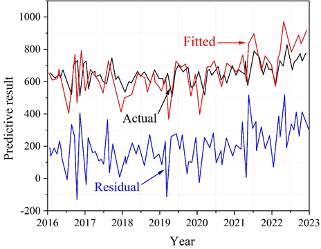
The effect of fitting the time series model to the sample observations is shown in Figure 3. It can be seen that there is a better match between the predicted value and the real value, and the fluctuation side and amplitude remain basically the same. The time series model predicted curve in 2018, 2019, 2020 appeared larger fluctuations, but keep the same fluctuation direction with the sample observations, the model fitting effect is better.
Eviews statistical analysis software was applied to analyze the raw data by multiple regression. The regression ANOVA is shown in Table 3. The F of the regression model is 1654.079, and its probability of significance is much less than 0.01. Therefore, the multiple regression model has a good fit to the data, and the regression model has a good overall effect.
| Model | Sum of Squares | df | Mean Square | F | p |
|---|---|---|---|---|---|
| Regression | 785108.611 | 25 | 31404.34444 | 1654.079 | 0.0000 |
| Residual | 65392.159 | 205 | 18.986 | / | / |
| Total | 850500.77 | 230 | / | / | / |
| Variable | Coefficient | Std. Error | t-Statistic | Prob. |
|---|---|---|---|---|
| C | 893.5221 | 97.624001 | 9.152688794 | 0.0000 |
| Price | -0.869550 | 0.168593 | -5.157687448 | 0.0000 |
| Advertising | 8.960751 | 0.218996 | 40.91741858 | 0.0000 |
| Substitution | -0.718993 | 0.187763 | -3.829258161 | 0.0000 |
| Complementarity | 7.986614 | 0.973142 | 8.207038644 | 0.0000 |
The regression coefficients and their tests are shown in Table 4, the regression coefficients of product price, advertising input, price of substitutes and price of complementary products on the sales volume are -0.869550, 8.960751 and -0.718993 respectively, and the significance probability level of each value is much less than 0.01. This indicates that all the influencing factors in the data have a significant effect on the sales volume of this product, and that the product’s own price and the price of substitutes are negatively correlated with sales, while advertising inputs and the price of complementary products are positively correlated with sales. This is basically in line with the economic and social reality, which shows that the model not only has a good fit and prediction accuracy, but also has a good practical application and interpretation ability.
After testing and analyzing the time series model and multiple regression model, the combination is synthesized and the results are calculated according to the principle of combination forecasting.
The fit of the combined model to the data is shown in Figure 4, which shows that the overall fit of the model to the data is better than that of the time series sub-model and the multiple regression sub-model, and it can be used for forecasting.The Residual value reaches a minimum in 2020 and is at [-100,0].

Comparing the prediction results of the combined model with the prediction results of the time series sub-model and the multiple regression sub-model, the prediction error of each prediction model can be obtained. Various prediction errors of the combined prediction model \(\varepsilon <max(\varepsilon _{1} ,\varepsilon _{2} )\), where \(\varepsilon\) indicates the prediction error of the combined model, \(\varepsilon _{1}\) indicates the prediction error of the time series sub-model, and \(\varepsilon _{2}\) indicates the prediction error of the multiple regression sub-model. \(max(\varepsilon _{1} ,\varepsilon _{2} )\) denotes the prediction error of the whole system of supply chain. Since the time series sub-model and the multiple regression sub-model are relative to a single enterprise, the prediction error of the whole supply chain system should take the larger of the sub-model prediction errors. As the combined forecasting model is relative to the whole supply chain system, the forecasting error of the combined forecasting model is much smaller than the forecasting error of the whole supply chain system.
The prediction effect evaluation indexes of each prediction model are shown in Table 5, and the variance of the prediction residuals of the time series sub-model and the variance of the prediction residuals of the multivariate regression sub-model can be obtained by calculation. The variance of the combined model prediction residuals is 2123.175.
Obviously, for the whole supply chain system, the variance of its prediction residuals, \(\delta <\frac{1}{2} max(\delta _{1} ,\delta _{2} )\). Based on the above analysis, it can be seen that the values of various error indicators of the sales combination prediction model based on are significantly lower than the maximum value of the error value of the single prediction model, thus indicating the superiority of the sales combination prediction method based on the accuracy is higher, and the sales prediction accuracy can be effectively improved.
| Prediction model | Mean absolute error (MAE) | Mean error (MSE) | Square sum error (SSE) | Mean absolute percentage error (MAPE) |
|---|---|---|---|---|
| Time sequence submodel | 87.26112 | 74.51361 | 507263.18 | 12.54348 |
| Multivariate regression submodel | 35.26997 | 36.24456 | 56.28034.31 | 3.52644 |
| Combination prediction model | 67.21569 | 48.01279 | 205739.48 | 2.67986 |
Setting an inventory cordon considers whether the inventory needs to be adjusted or not, and the classic formula for safety stock is used below to make an accurate calculation of the inventory of pharmaceuticals.
The influencing factors affecting safety stock mainly include uncertainty of consumer demand, instability of production process, changes in distribution cycle, and service level. Its calculation requires forecast data and historical demand data, according to the classic safety stock formula there: \[\label{GrindEQ__22_} SS=z*\overline{e_{d}^{2} +e_{i.}^{2} \left(d\right)^{2} } ,\tag{22}\] where \(SS\) is the safety stock.
The optimized safety stock equation: \[\label{GrindEQ__23_} SS=ze_{T} \overline{L/T} ,\tag{23}\] where \(\overline{L}\) is the average value of the lead time. Based on the predictions in this paper, it is useful to set a week as T = 7 days, and the formula can be converted to the following equation for the case where the lead time L is unchanged: \[\label{GrindEQ__24_} SS=ze_{K} \overline{L/7} ,\tag{24}\] where, \(e_{K}\) represents the standard deviation of weekly demand. And the weekly demand approximates the sales forecast as shown in Table 6, displaying as the occasion sales of the product in each week with the forecast value. As an example, the product inventory balance obtained for a product is 104 in December.
| Month | Period | First week | Second week | Third week | Fourth week | Total |
|---|---|---|---|---|---|---|
| January | Actual sales | 89 | 105 | 114 | 134 | 442 |
| Predictive value | 95 | 112 | 125 | 145 | 477 | |
| February | Actual sales | 124 | 130 | 132 | 155 | 541 |
| Predictive value | 150 | 166 | 165 | 201 | 682 | |
| March | Actual sales | 475 | 550 | 580 | 624 | 2229 |
| Predictive value | 412 | 470 | 512 | 597 | 1991 | |
| …… | …… | …… | …… | …… | …… | …… |
| December | Actual sales | 852 | 856 | 891 | 1025 | 3624 |
| Predictive value | 878 | 900 | 950 | 1000 | 3728 |
Calculate with the forecasted results. Next, this paper to act out the sales data of the first four weeks of each month to get the inventory balance of a product as an example. Assuming that the service level CSL = 99% and lead time L = 1, the sales data of January in the table as an example, using the formula in this paper, to get the safety stock value of \(SS_{January}\) each week. According to the statistical time of the remaining inventory and the actual sales of get the inventory balance of the cycle as shown in Table 7. The inventory balances for the 1st, 2nd, 3rd, and 4th weeks of January are 155, 167, 180, and 201, respectively.
| Period | First week | Second week | Third week | Fourth week |
|---|---|---|---|---|
| \(SS_{January}\) | 112 | 120 | 125 | 142 |
| \(SS_{January} /Actual\; sales\) | 0.7946 | 0.875 | 0.912 | 0.9437 |
| Inventory balance | 155 | 167 | 180 | 201 |
Enterprises can be guided by safety stock, when holding a high level of safety stock, then the balance of inventory can be used to meet the needs of later sales without the need to restock. In practice, managers have to make the right decision between high inventory and out-of-stock in order to effectively control inventory.
Retailer Company B, unlike the traditional manufacturing industry, does not have its own production and processing plant and can only purchase goods from manufacturers. Therefore, the procurement cost of purchasing products becomes a major component of Company B’s supply chain costs.
A comparison of the purchasing costs and gross margins of retailer Company B and manufacturer Company A is shown in Figure 5. Retailer Company B sells many categories of products and it is difficult to identify individual products for bookkeeping and accounting, so it is not possible to find the cost of the products purchased based on the categorization. Therefore, companies like Retailer B, Inc. generally use a combination of the cost of goods purchased plus a certain amount of gross profit to determine the selling price of the product, and do not add any other additional prices.
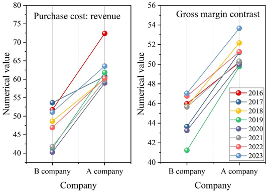
It can be noticed that when comparing Retailer B, Inc. and Manufacturer A from 2016-2023, Retailer B, Inc.’s share of purchasing costs has declined more significantly. It was 0.5175 in 2016 and decreased to 0.5107 in 2023. Indicating that the utilization of big data technology has effectively controlled the supply chain cost purchasing cost of Retailer B Company. The gross profit ratio of Retailer B also shows an increasing trend, which is 0.4598 in 2016 and grows to 0.5366 in 2023, indicating that its cost can be controlled and gross profit can be increased. Comparing with Manufacturer A, Retailer B Company has lower purchasing cost than Manufacturer A in the process of supply chain cost control using big data technology and it is effective.
The composition of operating costs of retailer Company B from 2016-2023 is shown in Figure 6, which shows that order processing expenses have always accounted for a larger share of operating costs, followed by technology research and development expenses, then sales and promotion expenses, and finally administrative expenses.
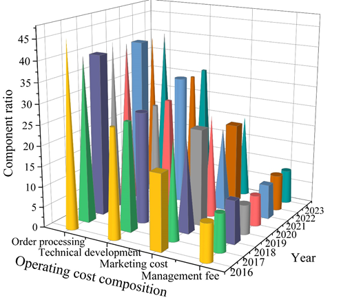
The amount of order processing costs in 2017-2023 shows a year-on-year decline, but its share of operating costs basically fluctuates up and down around 40%. Order processing cost is the main component of the operating cost of Retailer B, so it is necessary to control it by utilizing big data technology.
The proportion of marketing costs is basically showing an upward trend, and the amount is constantly rising, which has a lot to do with the expansion of Retailer B’s market share. The proportion of technology research and development expenses is maintained at 31% in both 2021 and 2023. After 2019, this proportion is basically rising and the amount is rising, which also proves that Retailer B is also increasing its investment in technology research and development.
The amount of administrative expenses shows a downward trend in 2019, although the amount has risen, the share of administrative expenses in operating costs is decreasing, which is inseparable from the relationship between Retailer B’s utilization of big data technology for supply chain cost control.
This paper designs a supply chain cost control program based on big data technology, unites CPFR theory, and constitutes an inventory optimization program for CPFR sales mix forecasting. It analyzes product demand, adjusts enterprise ordering, optimizes inventory resources, and realizes enterprise supply chain cost control.
The combined forecasting results are synthesized by combining the forecasting results of the time series model and the multiple regression model. For the whole supply chain system, the residual variance of the combined forecasting model is \(\delta <\frac{1}{2} max(\delta _{1} ,\delta _{2} )\). The estimation results of the CPFR-based sales combination forecasting model are more accurate and can effectively improve the sales forecasting accuracy.
The concept of safety stock is proposed, and the safety stock of the product cycle based on sales forecast is measured. In response to the inventory balance of the cycle, the enterprise carries out flexible ordering, adjusts the order quantity, and optimizes the supply chain link.
Comparing the effect of supply chain cost control between retailers and manufacturers, the gross profit margin percentage of the enterprise based on the CPFR sales mix forecasting model (i.e., retailer Company B) shows an increasing trend and grows to 0.5366 in 2023, which indicates that its cost can be controlled and its gross profit can be improved. Retailer Company B has reduced and effective purchasing costs in the process of supply chain cost control using big data technology.