
High-quality economic development is an inevitable requirement for China’s development to enter a new era, which is the unification of quantitative expansion and quality improvement of economic development. Promoting the coordinated development of regional economy is not only an important prerequisite for realizing complementary regional advantages, but also an important way to build a strong socialist modernized country [2, 18, 12]. China’s economy has shifted from the stage of high-speed growth to the stage of high-quality development, and there is an urgent need for new power support, and the rapid development of new-generation artificial intelligence and other digital industries has become a brand-new engine to promote the high-quality development of the economy. From “Made in China” to “Made in China”, AI has been applied in more and more R&D and scenarios, bringing great momentum to strategic emerging industry clusters [7, 30, 23]. Artificial intelligence has a profound impact on economic and social development through the use of information technology such as robots, computers, big data and the Internet [4].
However, the application of AI technology brings unprecedented challenges to the coordinated development of regions. China is a vast country, and there are certain developmental differences in the economy of each region under the influence of a variety of conditions [17, 1]. Maintaining moderate regional economic differentiation can bring into play the comparative advantages of each region and is the key to ensuring the effective functioning of the market mechanism, but the trend of regional economic imbalance continues to intensify, which will impose constraints on the high-quality development of the economy. Relying only on market mechanisms to promote technological progress often fails to maximize social welfare [15, 20]. In addition, with the updating and iteration of technology such as artificial intelligence, less developed regions may lose their resource and cost advantages, which in turn leads to the widening of the factor income distribution gap and the continued deepening of the trend of economic imbalance. Therefore, a comprehensive analysis of the impact of AI on regional economic development can help identify potential opportunities and obstacles, and put forward feasible countermeasure proposals to promote the sustainable development of AI technology and achieve strong regional economic growth [5, 27].
Meanwhile, the “Belt and Road” initiative has become an important platform for promoting regional economic development since its inception. Covering a wide geographical area and multiple economies, this initiative is intended to promote the integration and development of multiple economic regions in the countries along the route by strengthening infrastructure construction and enhancing regional connectivity [25, 19, 26]. However, while the “Belt and Road” promotes economic development, it also triggers a series of new economic and political challenges, which require regions to deal with unbalanced economic development, political and cultural differences, as well as the risk of capital investment, so as to turn the challenges into opportunities and realize high-quality development [14, 3, 9].
The progress of artificial intelligence technology promotes the development of social economy, and artificial intelligence technology promotes the efficient and low-cost development of social economy by supporting the national department’s economic development decision-making, promoting social governance, assisting the enterprise’s strategy formulation, and improving the efficiency of individuals’ work, etc. Gmeiner et al. [11] illustrated that the relevant responsible departments of the combination of artificial intelligence technology for the calculation of economic resources and allocation of the popular is still Can not fully achieve the market optimal efficiency and allocation, but artificial intelligence technology can effectively improve the market data acquisition efficiency, market incentives, etc.. Qin et al. [21] systematically searched the related research on AI technology empowering economic development, revealing that the research direction mainly involves intelligent decision-making, social governance, labor-management relations, and Industry 4.0 innovation, which provides an important reference for the research on AI for economic development. Ernst et al. [10] discussed that AI automation technology has provided a significant increase in the rate of economic development in the form of reduced production costs and increased productivity, and emphasized that inequality cannot be ignored while using AI technology to promote economic development, as well as focusing on security and protection in terms of data protection and data privacy. Raj et al. [22] based on economics and management research theories and perspectives, analyzed how artificial intelligence, automation technology affects the strategic development and organizational structure design of corporate economies, and contributed to the study of scholars and researchers related to corporate economic strategy and corporate organization.
Based on carbon‐inequality theory and regional data, Han et al. [13] found that Belt and Road economies have grown rapidly with investment, raising emissions, but their carbon‐emission inequality remains below the global average even as investment-driven inequality has risen; they propose regional mitigation and sustainability strategies. Chan [6] shows that multimodal transport and rail investments under the Belt and Road Initiative (BRI) have strengthened connectivity, boosted regional economies, and helped participating countries reduce marginalisation and poverty. Using Asian Development Bank data and a GTAP model, Yang et al. [29] report heterogeneous gains in growth, welfare, and trade across BRI countries, note some losses, and observe that the division of labour between developed and developing economies largely persists while China’s industrial upgrading benefits from BRI infrastructure. Together, these studies link the BRI to economic gains alongside uneven distributional and environmental consequences.
This paper determines the parameters of decision variables for optimal allocation of regional resources through the method of dividing regions, establishes the objective function in multi-objective optimization, and designs the regional resource allocation model of multi-objective optimization. The regional economic benefits and regional social benefits are targeted to maximize the direct benefits of regional economy. From the three aspects of resource availability, resource output capacity and regional coordinated development, the constraints of the model are proposed, and the constraints of each objective and variable are combined to complete the construction of the multi-objective overall model. According to the actual situation of the Belt and Road countries, the model is optimized by inputting the cooperative and orderly optimization model of the elemental composite system to achieve the optimal degree of coordination.
In the optimal allocation of regional resources, the decision variable parameters can be determined according to the characteristics of the research object by the method of dividing the region, that is, the region is divided into a number of sub-zones according to the topography, resource conditions, demand, etc. of the planning region [8]. If there are several resource supplies and several resource demands in each sub-area, the total number of decision variable parameters is the sum of the product of the number of resources and the number of demands in all sub-areas. In this way, the regional optimal resource allocation problem reduces to the optimal resource allocation problem of resources and demands within each sub-region. In this paper, the region is generalized to k partitions, the resource partition is generalized to i resources, and the demand is generalized to j demands.
The objective function of the regional resource allocation model based on multi-objective optimization adopts the general function of multi-objective optimization in operations research, which includes the main indicators of multi-objective optimization of regional resource allocation. Its function expression is as follows [24]: \[\label{GrindEQ__1_} \left\{\begin{array}{l} {MaxF(x)=Max\left[f_{1} (x),f_{2} (x),f_{3} (x),\cdots ,f_{n} (x)\right]}, \\ {MinF(x)=Min\left[f_{1} (x),f_{2} (x),f_{3} (x),\cdots ,f_{n} (x)\right]}, \\ {n=1,2,3,\cdots ,n}, \\ {s.t.:g_{i} (x)\le 0,x\ge 0}, \end{array}\right. \tag{1}\] where \(F(x)\) is the overall multi-objective variable, \(x\) is the decision variable, \(n\) is the number of optimization objectives, \(f_{1} (x),f_{2} (x),f_{3} (x),\cdots ,f_{n} (x)\) is the \(n\)th objective function, respectively, \(s.t.\) is the abbreviation of constraints, and \(g_{i} (x)\) is the \(i\)th constraint.
Maximize the direct economic benefits brought by the optimal allocation. The regional economic benefit objective function is as follows [16]: \[\label{GrindEQ__2_} Maxf_{1} (x)=\sum\limits_{k=1}^{k}\sum\limits_{j=1}^{N(k)}\left[\sum\limits_{i=1}^{M(k)}\left(b_{ij}^{k} -c_{ij}^{k} \right) x_{ij}^{k} \right] w_{k} , \tag{2}\] where \(Max_{1} (x)\) is the regional economic benefit target, \(b_{ij} {}^{k}\) represents the benefit per unit of resource \(i\) supplied to the \(j\)th user in Subarea \(k\), in yuan\(/{\rm m}^{3}\), \(c_{ij}^{k}\) represents the cost per unit of resource \(i\) supplied to the \(j\)th user in Subarea \(k\), in yuan\(/{\rm m}^{3}\), \(x_{ij}^{k}\) represents the amount of resource \(i\) supplied to the \(j\)th user in Subarea \(k\), in units of \({\rm m}^{3}\), \(w_{k}\) is the \(k\) zoning weighting coefficients.
For users, the most critical content of the social benefit objective of the optimal allocation of regional resources should be the part that best reflects the degree of user satisfaction with the effect of resources. Therefore, the objective of social benefit is reflected by adopting the total amount of missing resources in the region, that is, the size or degree of missing resources in the region. The regional social benefit objective function is as follows: \[\label{GrindEQ__3_} M\inf _{3} (x)=\sum\limits_{k=1}^{k}\sum\limits_{j=1}^{N(k)}\left[D_{j}^{k} -\sum\limits_{i=1}^{\mu _{ij} (k)}x_{ij}^{k} \right] , \tag{3}\] where \(M\inf _{3} (x)\) is the regional social benefit target, and \(D_{j}^{k}\) is the demand in units of \({\rm m}^{3}\) for the \(j\)th user in subarea \(k\).
Constraints on public resources [28] are, \[\sum\limits_{j=1}^{J(k)}x_{cj}^{k} \le D_{c}^{k} , \quad\,\,\,\sum\limits_{k=1}^{k}d_{c}^{k} \le W_{c},\] and constraints for independent resources are, \[\sum\limits_{j=1}^{J(k)}x_{cj}^{k} \le W_{i}^{k}\] where \(x_{cj}^{k}\) is the amount of supply from the public resource \(c\) to the \(j\)th user in the \(k\) zoning district, in units of \({\rm m}^{3}\), \(D_{c} {}^{k}\) is the amount of supply from the public resource \(c\) to the entire \(k\) zoning district, in units of 10,000 \({\rm m}^{3}\), \(W_{c}\) is the amount of supply available from the public \(c\) resource, and \(W_{i}^{k}\) is the amount of supply available from the independent resource \(i\) in the \(k\) zoning district.
Resource export capacity constraints are, \[\label{GrindEQ__4_} x_{ij}^{k} \le Q_{i}^{k} ;x_{cj}^{k} \le Q_{c} , \tag{4}\] where \(x_{ij}^{k}\) represents the amount of resource \(i\) supply to the \(j\)th user in Subarea \(k\) in units of \({\rm m}^{3}\), \(Q_{i}^{k}\) is the maximum conveyance capacity of resource \(i\) in Subarea \(k\) in units of \({\rm m}^{3} /{\rm s}\), \(x_{cj}^{k}\) is the amount of public resource \(c\) supply to the \(j\)th user in Subarea \(k\) in units of \({\rm m}^{3}\), and \(Q_{c}\) is the maximum conveyance capacity of public resource \(c\) in units of \({\rm m}^{3} /{\rm s}\).
Constraints to coordinated regional development are, \[\label{GrindEQ__5_} \mu =\sqrt{\mu _{B1} \left(\sigma _{1} \right)\mu _{B2} \left(\sigma _{2} \right)} \ge \mu ^{*} . \tag{5}\]
The affiliation functions \(\mu _{B1} \left(\sigma _{1} \right)\) and \(\mu _{B2} \left(\sigma _{2} \right)\) are the degree of coordination of fuzzy subsets of resource utilization and regional economic development, and the degree of coordination of economic development and environmental quality improvement, respectively.
The complete multi-objective regional resource optimization allocation model consists of a combination of regional economic benefit objectives, regional environmental benefit objectives, regional social benefit objectives, and constraints on each objective and variable: \[\label{GrindEQ__6_} F(x)=\left\{\begin{array}{l} {Maxf_{1} (x)=\sum\limits_{k=1}^{k}\sum\limits_{j=1}^{J(k)}\left[\sum\limits_{i=1}^{I(k)}\left(b_{ij}^{k} -c_{ij}^{k} \right) x_{ij}^{k} \right] w_{k} }, \\ {M\inf _{2} (x)=\sum\limits_{k=1}^{k}\sum\limits_{j=1}^{J(k)}0 .01d_{j}^{k} p_{j}^{k} \sum\limits_{i=1}^{I(k)}x_{ij}^{k} }, \\ {M\inf _{3} (x)=\sum\limits_{k=1}^{k}\sum\limits_{j=1}^{J(k)}\left[D_{j}^{k} -\sum\limits_{i=1}^{I(k)}x_{ij}^{k} \right] }. \end{array}\right. \tag{6}\]
The synergy degree of resource composite system measures the coordination level of mutual coordination and synergistic development of the resource input elements in the region, which is analyzed in depth through qualitative logical reasoning and quantitative data measurement, and the validity test proves the scientific validity of the synergistic measurement model for the study of the total economic output value, and the mathematical value of synergistic degree defined in this paper characterizes the economic development of the region in the current year. Therefore, the synergistic order optimization should be carried out by mathematical modeling with the primary purpose of keeping the synergistic degree robustly improved, so as to guarantee that the mathematical model has practical significance and research value.
Based on the above research and analysis, according to the actual situation of the countries along the Belt and Road, the synergistic and orderly optimization model of the compound system of resource input factors can be established, which can be used to carry out the optimal allocation of resources to achieve the highest degree of synergism and the best degree of coordination.
The mathematical expression of the specific optimization model and the meaning of the relevant identification codes are shown below: \[\label{GrindEQ__7_} \max f=CD_{t} ,t\in T , \tag{7}\] \[\label{GrindEQ__8_} CD_{t} \ge CD_{t-1} ,t\in T , \tag{8}\] \[\label{GrindEQ__9_} U_{i,t} \ge U_{i,t-1} ,i\in I,t\in T , \tag{9}\] \[\label{GrindEQ__10_} C_{t} \ge C_{t-1} ,t\in T , \tag{10}\] \[\label{GrindEQ__11_} \sum\limits_{t=1}^{n}I_{1,i} \ge A_{1,i} ,i=1,2,t\in T , \tag{11}\] \[\label{GrindEQ__12_} \sum\limits_{t=1}^{n}I_{2,2} \ge B,t\in T , \tag{12}\] \[\label{GrindEQ__13_} \sum\limits_{t=i}^{n}I_{3,i} \ge C_{3,i} ,i=1,2,4,t\in T , \tag{13}\] \[\label{GrindEQ__14_} \sum\limits_{t=1}^{n}I_{3,3} \le C_{3,3} ,t\in T , \tag{14}\] \[\label{GrindEQ__15_} x_{1,1,t} \ge x_{1,2,t} ,t\in T , \tag{15}\] \[\label{GrindEQ__16_} x_{1,2,t} \approx a_{t} , \tag{16}\] \[\label{GrindEQ__17_} x_{2,1,t} \le x_{2,2,t} ,t\in T , \tag{17}\] \[\label{GrindEQ__18_} x_{2,1,t} \approx b_{t} ,t\in T , \tag{18}\] \[\label{GrindEQ__19_} x_{3,i,t} \ge c_{i,t} ,1=1,2,4,t\in T , \tag{19}\] \[\label{GrindEQ__20_} x_{3,3,t} \le c_{3,t} ,t\in T . \tag{20}\]
The specific meanings of the optimization model identification codes for the input elements of economic resources are shown in Table 1. Through the above analysis, the optimization problem is firstly clarified, the optimization objective is clarified based on the understanding of the problem, after determining the objective, the constraints in two aspects are derived from the analysis based on the actual situation, accordingly, the optimization decision variables are selected, and these variables will be adjusted during the optimization process to achieve the optimal solution, and the overall logic of the optimization process is shown in Figure 1.
| \(CD_t \) | The system of the \(t\) year complex system is recognized |
| \(U_i,t \) | The first \(i\) subsystem is the order of the \(t\) year |
| \(C_t \) | The coupling degree of the \(t\) year subsystem |
| \(\sum\limits_i=1^nI_i,j \) | The first phase of the \(i\) subsystem is the time of the \(j\) optimization period Resource integration |
| \(x_i,j,t \) | The first number of the \(i\) subsystem is the \(j\) number of values in the year of \(t\) |
| \(X_i,j \) | The first \(i\) subsystem is the \(j\) policy constraint or the government’s expectations |
| \(a_t \) | The general public budget is expected to grow at \(t\) year |
| \(b_t \) | GDP is expected to grow in \(t\) year |

The following equation can be obtained from the objectives of regional economic benefits and regional social benefits: \[\label{GrindEQ__21_} \max f=\sqrt{\frac{(U_{fim} \times U_{lab} \times U_{mat} )(\alpha _{1} U_{fim} \times \alpha _{2} U_{lab} \times \alpha _{3} U_{mat} )}{(U_{fim} +U_{lab} )(U_{fim} +U_{mat} )(U_{lab} +U_{mat} )} } . \tag{21}\]
When the three subsystems of the composite system of economic resource input elements are in the same synergistic development, it can be assumed that the coupling degree of the three subsystems is at a consistent level, in order to simplify the process here assuming that the subsystems weight coefficients are the same, according to the above two assumptions, it can be obtained in the formula (22): \[\label{GrindEQ__22_} \max f=\sqrt{\frac{U_{fim} \times U_{lab} \times U_{mat} }{2} } . \tag{22}\]
Since \(U_{i} \in [0,1]\) and the subsystem orderliness measures do not affect each other, the objective function can be further decomposed to obtain the following equation: \[\label{GrindEQ__23_} \max f_{1} =U_{fim} , \tag{23}\] \[\label{GrindEQ__24_} \max f_{2} =U_{lab} , \tag{24}\] \[\label{GrindEQ__25_} \max f_{3} =U_{mat} . \tag{25}\]
According to the synergistic optimization model of regional economic resources, the optimization development results of regional economic resources are calculated. Figure 2 shows the optimization results of regional economic benefits and regional social benefits, and the analysis of Figure 2 shows that the development degree of each subsystem is showing a clear upward trend from 2017 to 2023, and it reaches the maximum value in 2023. It indicates that the economic development of the Belt and Road is moving forward in these years. The economic efficiency grows from 0.264 to 0.575, with a growth rate of 117.8%.
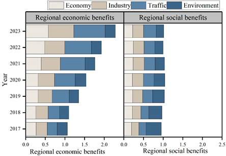
Through the regional economic resources synergistic optimization model, the optimization of social benefits corresponding to each subsystem in the Belt and Road region can be effectively defined, and the social benefit of the economic system grows from 0.196 to 0.224, with a growth rate of 14.29%.
Table 2 shows the index system of influencing factors. According to the previous review, the factors affecting the optimization of regional economic resources mainly include techno-economic factors, external factors, government intervention factors, infrastructure factors and industrial development factors. According to the actual situation of the “Belt and Road”, and considering the representativeness of the indexes and the availability of data, this paper selects the following indexes and factors to explore their effects on the optimization of regional economic resources in the countries along the route, including the proportion of medium- and high-technology exports, the proportion of merchandise trade, the inflow of foreign investment, the proportion of financial expenditures, and the mortality rate of road traffic, level of agricultural mechanization, and the share of industrial added value.
| Variable | Index | Index interpretation | Unit |
| Technical and economic factors | Medium and high technology exports(ME) | High technology exports account for the percentage of manufactured goods | % |
| External factor | Trade ratio(FT) | The total amount of trade in goods is a proportion of GDP | % |
| Foreign direct investment (FDI) | Capital inflow | Hundred million dollars | |
| Government intervention | Government expenditure ratio (FE) | Government spending on GDP | % |
| Infrastructure factor | Road traffic mortality (RTF) | The proportion of people killed by traffic accidents per 100,000 people | % |
| Agricultural machinery development index (AMDI) | In 2015, we measure the development of agricultural machinery | / | |
| Industrial development factor | Industry added value (PIA) | Industrial added value is the percentage of GDP | % |
The results of descriptive statistics of the variables concerned are shown in Table 3, from which it can be seen that the mean value of capital inflow is 946.158 and the standard deviation is 27631.396, which indicates a large deviation between the maximum and minimum values. The shares of medium and high technology exports, merchandise trade, government expenditure, road traffic mortality and industrial value added are 26.548%, 62.245%, 15.945%, 17.809% and 26.397% respectively.
| Variable | Unit | Mean | Standard deviation | Minimum value | Maximum value |
| Medium and high technology exports(ME) | % | 26.548 | 20.628 | 0 | 78.436 |
| Trade ratio(FT) | % | 62.245 | 28.926 | 8.396 | 164.563 |
| Foreign direct investment (FDI) | Hundred million dollars | 946.158 | 27631.396 | 0.000645 | 295000 |
| Government expenditure ratio (FE) | % | 15.945 | 5.395 | 2.054 | 39.565 |
| Road traffic mortality (RTF) | % | 17.809 | 7.948 | 2.396 | 41.265 |
| Agricultural machinery development index (AMDI) | / | 99.965 | 14.965 | 4.596 | 221.965 |
| Industry added value (PIA) | % | 26.397 | 10.796 | 6.624 | 75.954 |
The explanatory variable is the optimization of regional economic resources of the Belt and Road (RERO). Based on the previous relevant theoretical analysis, the model is constructed to build a panel data model: \[\label{GrindEQ__26_} RERO_{i,t} =\beta _{0} +\beta _{1} ME_{i,t} +\beta _{2} FT_{i,t} +\beta _{3} FDI_{i,t} +\beta _{4} FE_{i,t} +\beta _{5} RTF_{i,t} +\beta _{6} AMDI_{i,t} +\beta _{7} PIA_{i,t} +\varepsilon _{i,t} . \tag{26}\]
In order to ensure the smoothness of the variables and the correctness of the assessment, and to prevent pseudo-regression, the unit root test is performed before data regression. The unit root test is mainly summarized into two types: one contains the same unit root, and the test methods mainly include LLC, Breitungt-stat test, etc., and the other contains different unit roots, and the test methods mainly include IPS, ADF-Fisher test, etc. In this paper, we use three types of tests, LLC, IPS and ADF-Fisher test, Table 4 shows the unit root test, the P-value under the three tests is 0\(\mathrm{<}\)0.05, which indicates that the variables do not have a unit root and can be analyzed by panel regression. After the unit root test, all the variables test results are smooth, so there is no need to carry out the cointegration test for each factor.
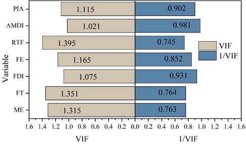
In this paper, when the indicators are selected from multiple perspectives for panel data regression, the regression of the model may be distorted due to the problem of multicollinearity among the influencing factors. Therefore, the Variance Inflation Factor (VIF) is used to test the seven explanatory variables, and Figure 3 shows the test of multicollinearity. The results show that the VIF values among the influencing factors are all much less than 10, with a mean value of 1.205, and the tolerance values (1/VIF) are all greater than 0.1, indicating that there is no multicollinearity among the indicators, and that the benchmark regression can be carried out.
| Variable name | LLC testing | IPS testing | ADP-Fisher testing | Test result | |||
|---|---|---|---|---|---|---|---|
| Statistic | P Value | Statistic | P Value | Statistic | P Value | ||
| RERO | -9.245 | 0.000 | -5.495 | 0.000 | 11.495 | 0.000 | Smoothness |
| ME | -13.455 | 0.000 | -8.526 | 0.000 | 19.168 | 0.000 | Smoothness |
| FT | -19.569 | 0.000 | -4.685 | 0.000 | 19.458 | 0.000 | Smoothness |
| FDI | -9.544 | 0.000 | -5.628 | 0.000 | 20.525 | 0.000 | Smoothness |
| FE | -8.265 | 0.000 | -3.948 | 0.000 | 14.685 | 0.000 | Smoothness |
| RTF | -15.955 | 0.000 | -8.859 | 0.000 | 18.678 | 0.000 | Smoothness |
| AMDI | -2.628 | 0.000 | -10.535 | 0.000 | 10.357 | 0.000 | Smoothness |
| PIA | -18.168 | 0.000 | -4.954 | 0.000 | 11.948 | 0.000 | Smoothness |
| Variable | Model 1(Mixing effect) | Mode 2(Fixed effect) | Mode 3(Random effect) | |||
| Coefficient | Standard error | Coefficient | Standard error | Coefficient | Standard error | |
| ME | 0.00049*** | 0.00008 | -0.00003 | 0.00007 | -0.00008 | 0.00007 |
| FT | 0.00018*** | 0.00004 | -0.00034*** | 0.00006 | -0.00024*** | 0.00004 |
| FDI | -0.00028*** | 0.00008 | -0.00015*** | 0.00004 | -0.00015*** | 0.00025 |
| FE | -0.00135*** | 0.00048 | 0.00023 | 0.00023 | 0.00006 | 0.00036 |
| RTF | 0.00006 | 0.00028 | -0.00285*** | 0.00035 | -0.00185*** | 0.00058 |
| AMDI | 0.00048 | 0.00009 | 0.000058** | 0.00048 | 0.0000965 | 0.000056 |
| PIA | -0.00182*** | 0.00028 | –0.00085*** | 0.00013 | -0.00125*** | 0.00025 |
| Constant term | 0.4126*** | 0.0048 | 0.4585 | 0.0089 | 0.4652*** | 0.0098 |
| Fixed effect VS hybrid effect | F testing | F=65.3125 | P=0.000 | |||
| Fixed effect VS stochastic effect | Hausman testing | x²=35.4544 | P=0.000 | |||
Before the panel regression analysis, the model used was judged by F test and Hausman test respectively. The results are shown in Table 5, with F=65.3125, x²=35.4544 and P-value of 0 for F-test and Hausman test, so the fixed effect model is used to analyze the factors influencing the optimization of regional economic resources in the Belt and Road environment.
According to the regression results of the fixed effect model (Model 2), it can be seen that there are five factors that have a significant impact on the optimization of regional economic resources in the countries along the route. Among them, four factors, namely, merchandise trade (-0.00034), foreign direct investment (-0.00015), road traffic mortality (-0.00285), and industrial development (0.00085), all have a negative effect at the 1% significant level, agricultural mechanization (0.000058) has a positive effect at the 5% significant level, and there is no significant relationship between the factors of medium and high technology and governmental financial expenditures significant relationship.
In order to further verify the reliability and consistency of the regression results of the factors influencing the optimization of regional economic resources, this paper will further carry out the robustness test. Examining the time lag effect of each factor, lagging each influencing factor by one period to get model 4. In order to avoid the influence of extreme values on the regression results, by shrinking the tail of each factor by 1% to get model 5. Considering the possible influence of the sample time and adjusting the stability of the regression results during the sample period, model 6 is obtained by eliminating the endpoint year. At the same time, taking into account the existence of spillover effects of regional economic resource optimization, that is, the optimization of regional economic resources may affect industrial development in the reverse direction, resulting in the existence of reverse causality between the two, causing endogeneity problems. Adopting the instrumental variable method, lagging the industrial value-added ratio by one period as the instrumental variable of the current industrial value-added, model 8 (the second stage regression results) is obtained through the two-stage least squares method. Table 6 shows the robustness test regression results, from the regression results in Table 6, the four factors of merchandise trade, foreign direct investment, road traffic fatality rate, and industrial development are all significantly negative, and the regression results of these four factors are -0.00026, -0.000078, -0.0028, -0.00169, and the agricultural mechanization are all significantly positive, as shown in the regression results of Model 8, for example. The regression results of each model are basically consistent with the benchmark regression results, indicating that the benchmark regression results are valid and reliable.
“There are significant differences in the per capita GDP, scientific and technological level, openness to the outside world and energy consumption structure of the countries along the Belt and Road, and under the green investment and trade rules, countries with a lower per capita GDP tend to adopt a crude growth approach to promote economic growth. Because these countries are still in the early stage of economic development, it is difficult to pay attention to environmental issues only by relying on market forces. Promoting the construction of green infrastructure is the first way to gradually transform their crude growth mode of “high input, high consumption and high emission”, build green supply chain systems, and promote their green transformation and upgrading. For countries with a low level of science and technology, green investment can be used to upgrade their level of science and technology and promote the intensive use of factor resources. Some of the countries along the border that mainly export resource-based products or have labor cost advantages and mainly engage in processing trade should take the approach of promoting their industrial and technological upgrading through green investment, so as to avoid these countries paying excessive resource and environmental costs in their development.
| Variable | Model 4 | Model 5 | Model 6 | Model 7 | Model 8 |
|---|---|---|---|---|---|
| ME | -0.00008 | -0.00002 | -0.00008** | -0.00035 | -0.000056 |
| (0.00078) | (0.000078) | (0.00005) | (0.000069) | (0.00004) | |
| FT | -0.00025*** | -0.00043*** | -0.00069*** | -0.00026*** | -0.00026*** |
| (0.000048) | (0.00004) | (0.00055) | (0.00036) | (0.000036) | |
| FDI | -0.00008** | -0.00027*** | -0.0018*** | -0.00012*** | -0.000078** |
| (0.00005) | (0.00003) | (0.00029) | (0.000036) | (0.00006) | |
| FE | -0.00028 | 0.00015 | -0.00092*** | -0.00048 | -0.00062 |
| (0.00029) | (0.00032) | (0.00028) | (0.00036) | (0.00039) | |
| RTF | -0.0028*** | -0.0023*** | -0.00025*** | -0.0026*** | -0.0028*** |
| (0.00026) | (0.00018) | (0.00023) | (0.00018) | (0.00036) | |
| AMDI | 0.00027*** | 0.00028*** | 0.00028*** | 0.00025*** | 0.000095** |
| (0.000058) | (0.000032) | (0.000049) | (0.00035) | (0.00003) | |
| PIA | -0.00078*** | -0.00085*** | -0.00078*** | -0.00097*** | -0.00169*** |
| (0.00026) | (0.00023) | (0.00016) | (0.00025) | (0.00036) | |
| Constant term | 0.4528*** | 0.4289*** | 0.4378*** | 0.4256*** | 0.4187*** |
| (0.0058) | (0.0028) | (0.0286) | (0.0265) | (0.0195) |
Promote and reshape the green governance cooperation model of countries along the “Belt and Road”. Reasonable environmental regulatory policies can effectively enhance the technological innovation capacity of regions and promote economic growth while reducing environmental pollution. On the basis of a green governance system that harmonizes domestic environmental protection with economic development, China should raise the greening threshold for export technologies and products and reshape the green governance cooperation model in accordance with the different levels of economic and social development of the “Belt and Road” countries. In cooperation with countries at a lower level of economic development, the level of fiscal expenditure of local governments should be appropriately increased through green investment and green financial cooperation, especially to strengthen green financial cooperation with the governments of such countries in the fight against environmental pollution. In cooperation with countries at a higher level of economic development, it is possible to introduce and exchange their respective green governance experiences through the establishment of green governance policy cooperation mechanisms. At the same time, according to the different levels of economic development of countries along the “Belt and Road”, promote the establishment of the “Belt and Road” environmental protection coordination mechanism, conduct performance evaluation of the level of sustainable development, and establish a green governance cooperation and consultation model in the green infrastructure construction and green investment of the “Belt and Road”.
Cooperation can be carried out through the green investment approach to promote technological efficiency through the continuous improvement of their production processes, taking the Made in China 2025 policy as an opportunity to internalize and embed the upgrading requirements and environmental standards of green transformation into the manufacturing process in China, and promote China’s green technology standards and green technology products to be promoted, so as to jointly enhance the level of sustainable development. Increase green technology cooperation, share green development technology experience, and combine with the existing cooperation mechanisms of international and regional organizations to establish a platform for information sharing and think tanks on sustainable development, so as to jointly negotiate and improve green technology standards, promote the joint enhancement of technological level, and give full play to the driving role of technological advancement in upgrading the level of sustainable development. While giving full play to its own comparative advantages, China also needs to actively introduce, digest and absorb advanced technologies from abroad, so as to continuously optimize the structure of its export products, increase the added value of its export products, and reduce the cost of its export products in terms of resources and the environment.
Using a multi-objective optimization function, this paper establishes a regional resource optimization allocation model, imposes constraints from three directions—resource availability, resource output capacity, and regional coordinated development—enhances the overall framework for multi-objective regional resource optimization, and analyzes regression results for factors affecting the optimization of economic resources. Through the regional economic resources synergistic optimization model, the optimization of regional economic and social benefits is quantified: the Belt and Road region’s economic system benefit rises from 0.196 to 0.224 (a 14.29% increase), while the degree of regional social benefit grows from 0.264 to 0.575 (a 117.8% increase), indicating a clear upward trend. According to fixed-effects regression results, the coefficients for merchandise trade, foreign direct investment, road traffic mortality, and industrial development are \(-0.00034\), \(-0.00015\), \(-0.00285\), and \(0.00085\), respectively, each statistically significant at the 1% level. A robustness test further verifies the reliability and heterogeneity of these results; taking model~8 as an example, the corresponding coefficients are \(-0.00026\), \(-0.000078\), \(-0.0028\), and \(-0.00169\), all showing negative correlations and consistent with the baseline analysis, indicating that the benchmark regression results are valid and reliable.