
In this note, we count the number of planted plane trees (also sometimes called ordered trees) on \(n\) nodes, each node is given a label from the set \(\{1, 2, \dots, k\}\), and labels must strictly decrease on any path from the root to a leaf. Let \(G_{n,k}\) denote this count for given positive integers \(n\) and \(k\). It is clear that \(G_{1,1} = 1\) and \(G_{n,1} = 0\) for all \(n \geq 2\). Then, letting \(C(n)\) denote the set of all compositions of \(n\), we have the recurrence formula \[\label{eq1} G_{n,k} = G_{n,k-1} + \sum_{S \in C(n-1)} \prod_{s \in S} G_{s,k-1}, \tag{1}\] for \(k \geq 2\). The first term \(G_{n,k-1}\) corresponds to the number of labellings that do not use the label \(k\). For the second term, the root label must be \(k\), the children of the root have subtrees with a total of \(n-1\) nodes, and each subtree must only use labels from \(\{1, 2, \dots, k-1\}\). Note that (1) is valid for \(n=1\) as well (with the summation equal to 1), since \(C(0) = {\emptyset}\). The sequence \(G_{n,k}\) has two parameters, which suggests the use of a bivariate generating function in its analysis (see, e.g., [12] for a detailed account of methods related to multivariate generating functions). However we found that the nature of our specific recurrence made it easiest to work with a sequence of single-variable generating functions instead. For \(k \geq 1\), let \(G_k(z)\) be the generating function \[G_k(z) = \sum_{n=1}^\infty G_{n,k} z^n.\]
Immediately we see that \(G_1(z) = z\), and from the recurrence (1), we have \[\label{eq2} G_k(z) = G_{k-1}(z) + \frac{z}{1 – G_{k-1}(z)}, \tag{2}\] for \(k \geq 2\). For any fixed \(k\) the function \(G_k(z)\) is rational, with nonnegative integers \(G_{n,k}\) as coefficients. Hence by Pringsheim’s theorem [4], if the radius of convergence of \(G_k(z)\) is \(R_k\), then \(R_k\) is a singularity of the function \(G_k(z)\). From the formula (2), it is clear that any pole of \(G_{k-1}(z)\) as well as any solution \(z\) to \(G_{k-1}(z) = 1\) is a pole of \(G_k(z)\).
For convenience, we define \(S_k(z) = 1 – G_k(z)\). The functions \(S_k(z)\) satisfy the recurrence \[\label{eq3} S_k(z) = S_{k-1}(z) – \frac{z}{S_{k-1}(z)}, \tag{3}\] with \(S_1(z) = 1 – z\). We define \(z^*_k\) to be the smallest positive real root of \(S_k(z)\); hence we must have \(S_k(z) > 0\) for \(z \in [0, z^*_k)\). Furthermore, the formula (3) implies that \(S_k(z) \leq S_{k-1}(z)\) for \(z \in [0, z^*_{k-1})\), so \(z^*_k\) is a nonincreasing sequence of positive numbers. We now give a lower bound for \(z^*_k\) and show that \(S_k(z)\) is small at a point close to this lower bound.
Lemma 1.1. For every \(k \geq 1\), \[\label{eq4} z^*_k \geq k – \sqrt{k^2 – 1}, \tag{4}\] and \[\label{eq5} S_k\left(\frac{1}{2k}\right) \leq \left(\frac{1}{4k}\right)^{1/4}. \tag{5}\]
Proof. Squaring both sides of (3) yields \[\label{eq6} S_k(z)^2 – S_{k-1}(z)^2 = -2z + \frac{z^2}{S_{k-1}(z)^2}, \tag{6}\] and by telescoping, we have \[\begin{aligned} \label{eq7} S_k(z)^2 &= (1 – z)^2 + \sum_{j=2}^k \left( S_j(z)^2 – S_{j-1}(z)^2 \right)\nonumber\\ &= (1 – z)^2 – 2(k-1)z + \sum_{j=2}^k \frac{z^2}{S_{j-1}(z)^2} \nonumber\\ &= 1 – 2kz + z^2 + \sum_{j=1}^{k-1} \frac{z^2}{S_j(z)^2}. \end{aligned} \tag{7}\]
Thus the lower bound \(S_k(z)^2 \geq 1 – 2kz + z^2\) is immediate, and since \(1 – 2kz + z^2\) is positive for \(0 \leq z < k – \sqrt{k^2 – 1}\), we must have \(z^*_k \geq k – \sqrt{k^2 – 1}\). This proves the first claim. From the bound just proved, we find that \(1/(2k) \in [0, z^*_k]\), so by our earlier observation, the sequence \(S_j\left(1/(2k)\right)\) is nonincreasing in \(j\). Moreover, we have \(S_j(z) \leq S_j(0) = 1\) for all \(j \geq 1\); from this we obtain \[\begin{aligned} \label{eq8} S_k\left(\frac{1}{2k}\right)^2 &= 1 – 2k \left(\frac{1}{2k}\right) + \left(\frac{1}{2k}\right)^2 + \sum_{j=1}^{k-1} \frac{1}{4k^2 S_j\left(1/(2k)\right)^2}\nonumber\\ & \leq \frac{1}{4k^2} + \frac{k-1}{4k^2 S_k\left(1/(2k)\right)^2}\nonumber\\ &\leq \frac{1}{4k S_k\left(1/(2k)\right)^2}. \end{aligned} \tag{8}\]
Solving the inequality gives \(S_k\left(1/(2k)\right) \leq \left(1/(4k)\right)^{1/4}\), as desired. ◻
Next, we derive an upper bound for \(z^*_k\).
Lemma 1.2. For all \(k \geq 1\), \[\label{eq9} z^*_k \leq \frac{1}{2k \left(1 – (1/(4k))^{1/4}\right)}. \tag{9}\]
Proof. First we observe that \(S_k\) is a concave function on \([0, z^*_k]\). This follows from the fact that \(G_k\) is a power series with positive coefficients and no constant term, so \(S_k = 1 – G_k\) has constant term 1 and all other coefficients negative. Moreover, as \(G_k\) is a rational function, it is analytic within its radius of convergence, hence all of its derivatives are well-defined and negative on \([0, z^*_k]\). Concavity of \(S_k\) gives us \[\label{eq10} S_k\left(\frac{1}{2k}\right) \geq \frac{1}{2kz^*_k} S_k(z^*_k) + \left(1 – \frac{1}{2kz^*_k}\right) S_k(0) = 1 – \frac{1}{2kz^*_k}, \tag{10}\] and applying Lemma 1 now yields \[\label{eq11} \left(\frac{1}{4k}\right)^{1/4} \geq 1 – \frac{1}{2kz^*_k}, \tag{11}\] and the result follows upon rearranging. ◻
We can now describe the first-order asymptotic behaviour of \(G_{n,k}\).
Theorem 1.3. Let \(G_{n,k}\) denote the number of planted plane trees with decreasing labels. Then for all \(k \geq 1\), there exist real numbers \(c_k\) and \(\alpha_k\) such that \[\label{eq12} G_{n,k} = c_k \alpha_k^n \left(1 + o(1)\right), \tag{12}\] as \(n \to \infty\), where \[\label{eq13} 2(k – 1)\left(1 – \frac{1}{\sqrt{2}(k-1)^{1/4}}\right) \leq \alpha_k \leq k – 1 + \sqrt{(k-1)^2 – 1}. \tag{13}\]
In particular, \(\alpha_k = 2k + o(k)\) as \(k \to \infty\).
Proof. As we did previously, for all \(k \geq 1\) let \(z^*_k\) denote the solution to \(G_k(z^k) = 1\). We know that for \(k \geq 2\), \(G_k(z)\) has only one pole on the domain \(|z| \leq z^*{k-1}\), namely, \(z^*_{k-1}\). We claim that this is a simple pole. Since \(G_1(z) = z\) and \[\label{eq14} G_k(z) = \frac{G_{k-1}(z)-G_{k-1}(z)^2 + z}{1 – G_{k-1}(z)}, \tag{14}\] for \(k \geq 2\), we see that \(G_k(z)\) is a rational function. Thus \[\label{eq15} \lim_{z \to z^*_{k-1}} (z – z^*_{k-1})G_k(z) = \frac{G_{k-1}(z^*_{k-1}) – G_{k-1}(z^*_{k-1})^2 + z^*_{k-1}}{-G'_{k-1}(z^*_{k-1})} = \frac{z^*_{k-1}}{-G'_{k-1}(z^*_{k-1})}. \tag{15}\]
The function \(G_{k-1}(z)\) is analytic on the domain \(|z| \leq z^{k-1}\) and its power series has nonnegative coefficients. Since the constant term in the power series \(G'{k-1}(z)\) is \[\label{eq16} [z] G_{k-1}(z) = G_{1,k-1} = k-1 > 0, \tag{16}\] the above limit is finite. This means that \(z^{k-1}\) is a pole of order 1 of the function \(G_k(z)\). Letting \(\alpha_k = 1/z^*{k-1}\), by a standard result on the coefficient asymptotics of rational functions, we have \[\label{eq17} G_{n,k} = c_k \alpha_k^n \left(1 + o(1)\right), \tag{17}\] where \(c_k\) is a constant depending on \(k\) only. The claimed bounds on \(\alpha_k\) follow from the two previous lemmas. ◻
We also note the following explicit upper bound. As \(G_k(z^*_k) = 1\), we immediately have \[G_{n,k} \leq \left(\frac{1}{z^*_k}\right)^n = \alpha_{k+1}^n.\] This is weaker than (17), but only slightly so, as \(\alpha_{k+1}/\alpha_k \to 1\) as \(k \to \infty\).
The regular leaning tree of order \(k\). Consider the sequence \(T_0, T_1, T_2, \dots\) of trees defined recursively as follows. Let \(T_0\) be a single root node with no children, and for \(k \geq 1\), we define \(T_k\) to be the tree with a root node having \(k\) children whose subtrees are \(T_{k-1}, T_{k-2}, \dots, T_0\). We shall call \(T_k\) the regular leaning tree of order \(k\). For all \(k \geq 0\), the tree \(T_k\) has \(2^k\) nodes. The following algorithm gives a mapping from the set of closed walks of length \(2n\) starting at the root of \(T_k\) and \(n\)-node planted plane trees with root label \(k+1\) and decreasing labels.
Algorithm 1.4 (Algorithm P).(Build planted plane tree). Given a closed walk \[\sigma = (u_0, u_1, \dots, u_{2n}),\] of length \(2n\) in \(T_k\), this algorithm outputs a planted plane tree labelled with positive integers.
Set \(i \leftarrow 0\) and initialize the tree \(P\) with a root node \(v\) and set \(\text{LABEL}(v) \leftarrow k+1\).
If \(u_{i+1}\) is the parent of \(u_i\), go to step P3. Otherwise, suppose that \(u_{i+1}\) is the root of a subtree isomorphic to \(T_j\) for some \(j < \text{LABEL}(v)\). Append a child with label \(j+1\) to \(v\) and update \(v\) to point to this child. Go to step P4.
Set \(v \leftarrow \text{PARENT}(v)\).
Increment \(i\) by one. If \(i < 2n\), go to step P2; otherwise terminate the algorithm with the tree \(P\) as output.
The root of the output planted plane tree has label \(k+1\), and every time we move downward in \(T_k\) along the path \(\sigma\) and encounter the root of \(T_j\) for some \(j \leq k\), we append a node with label \(j+1\). This implies that the output of Algorithm P is a planted plane tree with decreasing labels and root label \(k+1\). We also know that this output tree has \(n+1\) nodes, since we start with one root node, and in the walk \(\sigma\), half of the \(2n\) edges must go down in the tree and half must go up (to return to the root), and we add a node to \(P\) when (and only when) going down. The tree \(P\) is built up in depth-first preorder, so it is easy to write an algorithm that recovers the walk from a tree \(P\) output by Algorithm P.
Algorithm 1.5 (Algorithm W).(Build walk in \(T_k\)). Given a planted plane tree \(P\) with decreasing labels and root label \(k+1\), we build a walk \(\sigma\) starting at the root in \(T_k\). Suppose we have a function \(\text{NEXT}(v)\) of getting the node that follows a given node \(v \in P\) in a depth-first traversal of \(P\) (in this traversal, nodes may be visited multiple times).
Let \(u_0\) be the root of \(T_k\). Set \(i \leftarrow 0\) and let \(v\) be the root of \(P\).
Let \(w \leftarrow \text{NEXT}(v)\). If \(w\) is the parent of \(v\), go to step W3. Otherwise, let \(u_{i+1}\) be the child of \(u_i\) that is the root of the subtree isomorphic to \(T_j\), where \(j = \text{LABEL}(w) – 1\). Go to step W4.
Set \(u_{i+1} \leftarrow \text{PARENT}(u_i)\).
Set \(v \leftarrow w\) and increment \(i\) by one. (An invariant we have maintained is that \(u_i\) is the root of a subtree isomorphic to \(T_j\), where \(j = \text{LABEL}(v) – 1\). This makes step W2 possible in the next iteration.) If \(i < 2n\), go to step W2; otherwise, terminate the algorithm with output \(\sigma = (u_0, u_1, \dots, u_{2n})\).
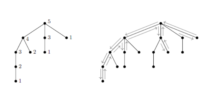
An example of a tree \(P\) and its corresponding walk in \(T_k\) is illustrated in Figure 1. The parallel structures of Algorithms P and W make it clear that if Algorithm P terminates with output \(P\) upon being given input \(\sigma\), then Algorithm W returns the walk \(\sigma\) upon the input \(P\). We have thus furnished a bijective proof of the following theorem.
Theorem 1.6. Let \(n\) and \(k\) be positive integers. The number \(W_{2n}(T_k)\) of closed paths in \(T_k\) of length \(2n\) that begin and end at the root is equal to the number \(G_{n+1,k+1} – G_{n+1,k}\) of \((n+1)\)-node planted plane trees with decreasing labels and root label equal to \(k+1\).
The top eigenvalue of a regular leaning tree. Let \(\Gamma = (V, E)\) be a connected graph, let \(A = A(\Gamma)\) be its adjacency matrix, and let \(\lambda_1(A)\) denote the largest eigenvalue of \(A\). By the trace method, we have \[\begin{aligned} \label{eq18} \lambda_1(A) &= \lim_{n \to \infty} \left( \operatorname{tr} (A^{2n}) \right)^{1/2n}\nonumber\\ &= \lim_{n \to \infty} \left( \max_{v \in V} W_{2n}(v, \Gamma) \right)^{1/2n}\nonumber\\ &= \lim_{n \to \infty} \left( \min_{v \in V} W_{2n}(v, \Gamma) \right)^{1/2n}, \end{aligned} \tag{18}\] where \(W_{2n}(v, \Gamma)\) denotes the number of closed walks of length \(2n\) in \(\Gamma\) starting at the vertex \(v\). It is well known that if \(\Gamma = T\) is a tree and \(A\) is its adjacency matrix, then the largest eigenvalue \(\lambda_1(A)\) of \(A\) satisfies \[\label{eq19} \sqrt{\Delta} \leq \lambda_1(A) \leq 2 \sqrt{\Delta – 1}, \tag{19}\] where \(\Delta \geq 2\) is the maximum vertex degree of \(T\). (The lower bound is trivial and the upper bound is a result of D. Stevanovi’c [13].) Theorems 3 and 4 together tell us that largest eigenvalue of the adjacency matrix of a leaning tree of order \(k\) (which has maximum vertex degree \(k+1\)) does not tend towards either of these bounds as \(k \to \infty\).
Lemma 1.7. Let \(k \geq 1\) and let \(A_k\) denote the adjacency matrix of the regular leaning tree \(T_k\). Then the largest eigenvalue \(\lambda_1(A_k)\) is \(\sqrt{2k + o(k)}\).
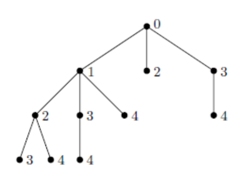
The Ulam–Harris number. We can extend the above result to arbitrary trees as follows. We give the root the label 0, and for any node with label \(r\) and \(s\) children, we label the children \(r+1, r+2, \dots, r+s\). We define the Ulam–Harris number UH\((T)\) of a planted plane tree \(T\) to be the maximum label in the tree. (There is a standard notion of the Ulam–Harris labelling of a tree (see, e.g., Section 6 of [5]), in which one assigns a vector of positive integers to each node. Our Ulam–Harris number is the maximum sum of coordinates, taken over all Ulam–Harris labels in the tree.) For an unordered tree \(T\), we can let UH\((T)\) be the minimum of UH\((T')\) over all planted plane trees \(T'\) obtained from \(T\) by choosing orderings for the children of each node.
Theorem 1.8. Let \(T\) be a rooted unordered tree, and let \(A\) be the adjacency matrix of \(T\). Then \(\lambda_1(A) \leq \lambda_1(A_{\operatorname{UH}(T)})\), where \(A_{\operatorname{UH}(T)}\) is the adjacency matrix of the regular leaning tree of order UH\((T)\).
Proof. Consider \(T\) as a labelled planted plane tree, with maximum label UH\((T)\). Replace each label \(j\) with UH\((T) – j\). Then the root has label UH\((T)\), all labels are nonnegative and decreasing both as one descends in the tree, and as one goes from left to right among siblings. Furthermore, the new label of each node is strictly greater than the number of children it has, so we can embed \(T\) into the regular leaning tree \(T_{\operatorname{UH}(T)}\), and the claim follows. ◻
Let \(T\) be a tree with maximum vertex degree \(\Delta\) and adjacency matrix \(A\). Since a node and its children must all have different labels, we must have UH\((T) \geq \Delta\); the regular leaning tree of order \(k\) attains this bound with equality. Lemma 1.7 and Theorem 1.8 together supply an upper bound of roughly \(\sqrt{2 \operatorname{UH}(T)}\) on \(\lambda_1(A)\). In the scenario where UH\((T) < 2\Delta – 2\) (as in Figure 2, for instance), this improves upon Stevanovi’c’s bound of \(2\sqrt{\Delta – 1}\).
In this paper we have considered trees with decreasing labels, but in the literature it has been somewhat more common to count trees with increasing labels (by reflecting the values of the nodes, there are exactly as many increasing trees with maximum label \(k\) as there are decreasing ones). There is a classical bijection between permutations of \({1, \dots n}\) and increasing binary trees on \(n\) nodes using each label from 1 through \(n\) exactly once. A 2020 paper of Bodini et al. [2] relaxed the stipulation that all the labels 1 through \(n\) must appear, requiring instead that for some \(1 \leq k \leq n\), all the labels 1 through \(k\) must appear (labels must still strictly increase down the tree). A later paper of Bodini et al. [3] describes a more general approach that applies to more families of trees.
In 1987, Blieberger [1] counted the number of Motzkin trees with labels that increase, but not necessarily strictly. Kemp showed in 1993 [7] that the planted plane trees labelled similarly are in bijection with monotonically extended binary trees. In 2011, Janson, Kuba and Panholzer [6] drew a link between generalized Stirling permutations and \(k\)-ary trees with (strictly) increasing labels. A generalization of labelled trees, in which nodes can receive multiple labels, was introduced in 2016 by Kuba and Panholzer [10] and this generalization is shown to imply various hook-length formulas for trees.
Other authors have considered the average shape [8] and the degree distribution [9] of various tree families with increasing labels. The expectation and variance of the size of the ancestor tree as well as the Steiner distance of increasingly labelled trees were determined by Morris in 2004 [11].
We thank Ari Blondal, G’abor Lugosi, and Steve Melczer for stimulating discussions and helpful suggestions. We are also grateful for the anonymous referee’s corrections and comments, which helped us improve the readability of the paper. The second and third authors are funded by the Natural Sciences and Engineering Research Council of Canada.