
Let \(G\) be a plane graph with vertex, edge, and region sets \(V(G), E(G), F(G)\) respectively. A zonal labeling of a plane graph \(G\) is a labeling \(\ell: V(G)\rightarrow \{1,2\}\subset \mathbb{Z}_3\) such that for every region \(R\in F(G)\) with boundary \(B_R\), \(\sum\limits_{v\in V(B_R)}\ell(v)=0\) in \(\mathbb{Z}_3\). We call the value \(\sum\limits_{v\in V(B_R)}\ell(v)\) the label of \(R\), and denote this \(\ell(R).\) We can then equivalently state that a labeling \(\ell:V(G)\rightarrow \{1,2\}\) is zonal if and only if the induced labeling \(\ell: F(G)\rightarrow\mathbb{Z}_3\) assigns the label \(0\) to every region. A plane graph is zonal if it admits a zonal labeling.
Given a vertex \(v\in V(G),\) we let \(X_v=\{R\in F(G): v\in V(B_R)\}\) denote the set of regions with \(v\) on their boundary. A cozonal labeling of a plane graph \(G\) is a labeling \(\ell^*: F(G)\rightarrow \{1,2\}\subset \mathbb{Z}_3\) such that for all \(v\in V(G),\) \(\sum\limits_{R\in X_v}\ell^*(R)=0\). We call the value \(\sum\limits_{R\in X_v}\ell^*(R)\) the label of \(v\), and denote this \(\ell^*(v).\) We can equivalently state that a labeling \(\ell^*:F(G)\rightarrow \{1,2\}\) is cozonal if and only if the induced labeling \(\ell^*:V(G)\rightarrow \mathbb{Z}_3\) assigns the label \(0\) to every vertex. A plane graph is cozonal if it admits a cozonal labeling. Other terms not specifically defined here are standard and can be found in texts such as [7].
Zonal labelings were first introduced by Cooroo Egan in 2014 (see [5]) to study the Four Color Theorem. In particular, zonal labelings were studied in connection with a special kind of plane graph called a cubic map. A cubic map is a \(2\)-connected cubic plane graph. There is a connection between zonal labelings of cubic maps and edge \(3\)-colorings of cubic maps. The following fact is proven in [5, 6]:
Theorem 1.1. Let \(M\) be a cubic map. Then \(M\) has a proper edge \(3\)-coloring if and only if \(M\) admits a zonal labeling.
In 1880, Peter Tait proved that a cubic map has a proper edge \(3\)-coloring if and only if it has a proper region \(4\)-coloring [9]. Therefore, a key result follows [5, 6]:
Theorem 1.2. Let \(M\) be a cubic map. Then \(M\) has a proper region \(4\)-coloring if and only if \(M\) admits a zonal labeling.
In 1976 it was proven that every plane graph admits a proper region \(4\)-coloring, resulting in the famous Four Color Theorem (see [1, 8]). Therefore, every cubic map is zonal. Furthermore, showing that every cubic map is zonal independently of the Four Color Theorem would constitute a new proof of the Four Color Theorem. In order to gain a new perspective on zonal labelings, cozonal labelings were introduced in [2]. Based on the definition of cozonal labelings, there is an important dual relationship between zonality and cozonality. The following is proven in [3]:
Proposition 1.3. A connected plane graph \(G\) is zonal if and only if its plane dual \(G^*\) is cozonal.
Therefore, there is a nice dualization of Theorem 1.1. A plane triangulation is a plane graph where the boundary of every region is a triangle. The dual of a cubic map is a plane triangulation, and vice versa. The dualization of an edge \(3\)-coloring of a cubic map is a tricoloring of a plane triangulation \(T\), in which the edges of \(T\) are colored with three colors such that each color appears on the boundary of each region. The theorem below is proven in [2] using properties unique to cozonal labelings.
Theorem 1.4. Let \(T\) be a plane triangualtion. Then \(T\) has a tricoloring if and only if \(T\) admits a cozonal labeling.
While the choice of the group \(\mathbb{Z}_3\) for our labels is deeply connected with the study of the Four Color Theorem, there is certainly no reason why we cannot use elements from other groups as our labels. Let \(\Gamma\) be a nontrivial abelian group with identity element \(0\). We will use additive notation for group elements. We can naturally generalize the definitions of zonal and cozonal to groups other than \(\mathbb{Z}_3.\) We therefore define a \(\Gamma\)-zonal labeling of a plane graph \(G\) as a labeling \(\ell:V(G)\rightarrow \Gamma\setminus \{0\}\) such that for every region \(R\in F(G)\) with boundary \(B_R\), the induced label \(\ell(R)=\sum\limits_{v \in V(B_R)}\ell(v)\) is \(0\). We define \(\Gamma\)-cozonal analogously. We will explore several results on these generalized labelings, as well as introduce two additional restrictions that lead to many possible new questions.
Before looking at specific graphs, let us observe a few basic relations between \(\Gamma\)-zonal labelings with related groups. We will state our observations in terms of \(\Gamma\)-zonality only for brevity.
Observation 2.1. Let \(G\) be a plane graph, and let \(\Gamma \le \Gamma'\) be abelian groups. If \(G\) is \(\Gamma\)-zonal, then \(G\) is \(\Gamma'\)-zonal.
Observation 2.2. Let \(G\) be a plane graph, let \(\Gamma\) and \(\Gamma'\) be abelian groups, and let \(\varphi:\Gamma\rightarrow \Gamma'\) be a group homomorphism. If \(\ell:V(G)\rightarrow \Gamma \setminus \ker(\varphi)\) is a \(\Gamma\)-zonal labeling, then \(\varphi(\ell)=\varphi\circ \ell\) is a \(\Gamma'\)-zonal labeling.
Proof. Since no vertex has a label in \(\ker(\varphi)\), it follows that \(\varphi(\ell)\) assigns vertices labels from \(\Gamma'\setminus\{0\}\). Since \(\varphi\) is a group homomorphism, addition is preserved, and the induced label of each region is \(0\) in the new group. ◻
In the study of zonal (and cozonal) labelings where our group is \(\mathbb{Z}_3\), we use \(\bar \ell\) to refer to the complimentary labeling defined by the relation \(\bar \ell(v) =2\ell(v)\). We see that Observation 2.2 generalizes complimentary labelings. However, there is one difference. In the case of zonal labeling, we can use complimentary labelings to assume without loss of generality that in a zonal labeling \(\ell\) the label of a certain vertex \(v\) is \(1\). This is because if \(\ell(v)=2\), we simply take the complimentary labeling to obtain a zonal labeling where the label is \(1\) instead. If our group is for instance \(\mathbb{Z}_4\), we cannot make such an assumption. As an example, there is no endomorphism \(\varphi\) such that \(\varphi(2)=1.\) Alternatively, an endomorphism that maps \(\varphi(1)=2\) may map some other labels to \(0\), resulting in a labeling which is not \(\mathbb{Z}_4\)-zonal. While automorphisms of \(\Gamma\) can be used to reduce the number of possible labels of a vertex, we cannot generally make the assumption that a single vertex has a specific label.
We will primarily restrict our attention to \(2\)-connected graphs. We begin with the simplest possible \(2\)-connected graph: the cycle \(C_n\). First, the matter of \(\Gamma\)-cozonal labelings is trivial; labeling one region with any nonzero element \(g\in \Gamma\) and the other with its inverse \(-g\) is a \(\Gamma\)-cozonal labeling, as the induced label of each vertex is \(g-g=0.\) Therefore such labelings exist for all \(\Gamma\).
Next, we will find that while slightly less trivial, it is still easy to obtain \(\Gamma\)-zonal labelings of \(C_n\). First, we obtain a brief but useful lemma.
Lemma 2.3. Let \(\Gamma\not \simeq\mathbb{Z}_2\) be an abelian group. Then \(\Gamma\) contains three nonzero elements \(g_1, g_2, g_3\) (not necessarily distinct) such that \(g_1+g_2+g_3=0.\)
Proof. Begin by choosing an arbitrary nonzero element \(g_1\in \Gamma\), and let \(g_2\in \Gamma\setminus\{0, -g_1\}.\) This set is nonempty as long as \(\Gamma \not \simeq \mathbb{Z}_2\). Finally, let \(g_3=-(g_1+g_2)\). Since \(g_2\ne -g_1,\) it follows that \(g_1+g_2\ne 0\). Therefore, \(g_1, g_2, g_3\) are nonzero, and \[g_1+g_2+g_3=g_1+g_2-(g_1+g_2)=0.\] ◻
With this lemma, we proceed.
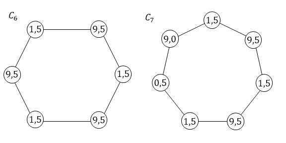
Proposition 2.4. Let \(C_n\) be a cycle with \(n\ge 3\), and let \(\Gamma\) be an abelian group. Then \(C_n\) has a \(\Gamma\)-zonal labeling in all cases except when \(\Gamma\simeq \mathbb{Z}_2\) and \(n\) is odd.
Proof. We note that when \(\Gamma\simeq\mathbb{Z}_2\), the only available label is \(1\). Assigning \(1\) to each vertex produces a \(\Gamma\)-zonal labeling if and only if \(n\) is even. Thus, there is no \(\mathbb{Z}_2\)-zonal labeling when \(n\) is odd.
Now let \(\Gamma \not \simeq \mathbb{Z}_2\). If \(n\) is even, we choose a nonzero element \(g\in \Gamma\), assign half the vertices the label \(g,\) and assign the other half the label \(-g\). Then the induced label of each region is \((n/2)g-(n/2)g=0\), and the labeling is \(\Gamma\)-zonal. Next, we consider \(n=2n'+1\) odd. When \(\Gamma\not \simeq \mathbb{Z}_2\), then there are three nonzero elements \(g_1, g_2, g_3\) such that \(g_1+g_2+g_3=0\). Therefore, we assign \(n'-1\) vertices some nonzero element \(g,\) \(n'-1\) vertices the element \(-g\), and the remaining three vertices \(g_1, g_2, g_3\) respectively. Then the label of each region is \((n'-1)g-(n'-1)g+g_1+g_2+g_3=0.\) This is therefore a \(\Gamma\)-zonal labeling of \(C_n\). ◻
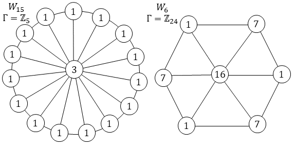
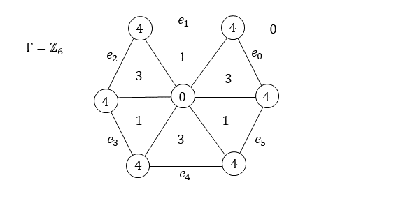
In Figure 1 we give examples of \(\Gamma\)-zonal labelings of \(C_6\) and \(C_7\). Next we turn to another simple class of graphs. Let \(W_n\) denote the wheel \(C_n \vee K_1.\) The wheel is interesting as it is self-dual; therefore we may explore the concepts of \(\Gamma\)-zonality and \(\Gamma\)-cozonality simultaneously. It was shown in [4] that \(W_n\) is zonal (and therefore cozonal) if and only if \(n\equiv 0 \pmod 3.\) However, by changing our group \(\Gamma\) we are able to obtain \(\Gamma\)-zonal labelings of \(W_n\). In fact, we can obtain a complete characterization. We will divide this characterization into two parts based on the parity of \(n\).
Proposition 2.5. Let \(\Gamma \not \simeq \mathbb{Z}_2\) be an abelian group, and let \(n\ge 4\) be even. Then \(W_n\) has a \(\Gamma\)-zonal labeling if and only if \(\Gamma\) has an element \(g\) of order \(k\ge 2\) such that \(k\) divides \(n/2\).
Proof. Let the outer cycle \(C_n\) be given by \((v_0, v_1,…, v_{n-1}, v_0)\) with subscripts given in \(\mathbb{Z}_n\), and let the central vertex be \(u.\) Suppose \(\ell\) is a \(\Gamma\)-zonal labeling. Then for each \(i\in \mathbb{Z}_n\), there are regions with boundaries \((u, v_{i}, v_{i+1}, u)\) and \((u, v_{i+1}, v_{i+2}, u).\) Therefore, \(\ell(v_i)=\ell(v_{i+2})\) for all \(i\), and the boundary of the exterior region is equal to \((n/2)(\ell(v_0)+\ell(v_1))\). Thus the additive order of \(\ell(v_0)+\ell(v_1)\) divides \(n/2.\) Moreover, \(\ell(v_0)+\ell(v_1)\ne 0\), as otherwise the label of each triangular region would be \(\ell(u)\ne 0\). Therefore the additive order of \(\ell(v_0)+\ell(v_2)\) is at least \(2\), and the desired element exists.
Next, assume \(\Gamma\) is a group with an element \(g\in \Gamma\) with order \(k\ge 2\) such that \(k\) divides \(n/2\). Choose an element \(g' \in \Gamma \setminus \{0, g\}\); since \(\Gamma \not \simeq \mathbb{Z}_2\), such an element exists. Consider the labeling given by \(\ell(v_i)=g'\) if \(i\) is even, \(\ell(v_i)=g-g'\) if \(i\) is odd, and \(\ell(u)=-g.\) Then the label of each triangular region is \(g'+(g-g')-g=0\), and the label of the exterior region is \((n/2)(g'+(g-g')) = (n/2)g=0.\) ◻
Proposition 2.6. Let \(\Gamma \not \simeq \mathbb{Z}_2\) be an abelian group, and let \(n\ge 3\) be odd. Then \(W_n\) has a \(\Gamma\)-zonal labeling if and only if \(\Gamma\) has an element \(g\) of order \(k\ge 3\) such that \(k\) divides \(n\).
Proof. Begin with the construction in Proposition 2.5, and suppose \(\ell\) is a \(\Gamma\)-zonal labeling. As in the even case, \(\ell(v_i)=\ell(v_{i+2})\) for all \(i\). However, this then implies that all vertices on \(C_n\) have the same label. Thus the boundary of the exterior region is \(n\ell(v_0)=0\), and the order of \(\ell(v_0)\) divides \(n\). Moreover, \(\ell(v_0)\) cannot have order \(1\) or \(2\), as otherwise the boundary of each triangular region would be \(\ell(u)\ne 0\) (and moreover, \(2\) does not divide \(n\)).
Next, suppose that \(\Gamma\) has an element \(g\) of order \(k\ge 3\) such that \(k\) divides \(n\). Let \(\ell(v_i)=g\) for all \(i\) and let \(\ell(u)=-2g\). Then the label of each triangular region is \(g+g-2g=0\), and the label of the exterior region is \(ng=0.\) ◻
We will display examples of \(\Gamma\)-zonal labelings of wheels in Figure 3. Next we will look at some larger categories of graphs. We start with \(2\)-connected bipartite plane graphs. These were found to be zonal in [4]. In fact, the same strategy applies more generally.
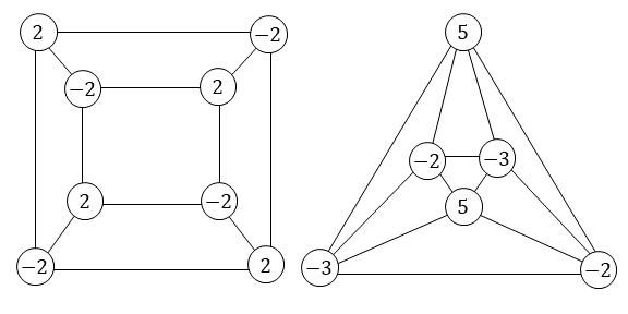
Proposition 2.7. Let \(\Gamma\) be an abelian group. If \(G\) is a \(2\)-connected bipartite plane graph, then \(G\) is \(\Gamma\)-zonal. Dually, if \(G\) is a \(2\)-connected Eulerian plane graph, then \(G\) is \(\Gamma\)-cozonal.
Proof. We will prove the statement on \(\Gamma\)-zonality. Since \(G\) is bipartite, the vertices of \(G\) have a proper \(2\)-coloring \(f:V(G)\rightarrow\{1,2\}\). Let \(g\in \Gamma\) be nonzero, and form the labeling \(\ell:V(G)\rightarrow \Gamma\setminus \{0\}\) given by \(\ell(v)=g\) if \(f(v)=1\) and \(\ell(v)=-g\) otherwise. Consider a region \(R\in F(G)\). Since \(G\) is bipartite, the boundary of \(R\) is an even cycle, and since \(f\) is a \(2\)-coloring, half the labels on the boundary of \(R\) are \(g\) and the other half are \(-g.\) These labels sum to \(0\), and therefore \(\ell(R)=0.\) Thus, \(\ell\) is a \(\Gamma\)-zonal labeling. ◻
Next we turn to another category of graphs which produces a similarly nice result.
Proposition 2.8. Let \(\Gamma \not \simeq \mathbb{Z}_2\) be an abelian group. If \(G\) is an Eulerian plane triangulation, then \(G\) is \(\Gamma\)-zonal. Dually, if \(G\) is a bipartite cubic map, then \(G\) is \(\Gamma\)-cozonal.
Proof. We will prove the statement on \(\Gamma\)-zonality. Let \(G\) be an Eulerian plane triangulation. Since \(\Gamma \not \simeq \mathbb{Z}_2\), there exist three nonzero elements \(g_1, g_2, g_3\) of \(\Gamma\) which sum to \(0\). In addition, since \(G\) is an Eulerian plane triangulation, then the vertices of \(G\) have a proper \(3\)-coloring \(f:V(G)\rightarrow \{1,2,3\}\). Form the labeling \(\ell:V(G)\rightarrow \Gamma\) given by \(\ell(v)=g_{f(v)}\). Since the boundary vertices of each region are mutually adjacent, they receive distinct colors under \(f\), and therefore each region \(R\in F(G)\) has elements \(g_1, g_2, g_3\) on its boundary. Therefore \(\ell(R)=0\) for all \(R\in F(G)\), and \(\ell\) is a \(\Gamma\)-zonal labeling. ◻
Examples of \(\Gamma\)-zonal labelings of \(2\)-connected bipartite plane graphs and Eulerian triangulations are given in Figure 2. We close this section by briefly discussing nonexistence of \(\Gamma\)-zonal labelings (and dually, \(\Gamma\)-cozonal labelings). Let \(G\) be a \(2\)-connected plane graph such that there are two regions \(R_1, R_2\) with boundary cycles \(B_1, B_2\) where \(V(B_1)=V(B_2)\cup \{v\}\) for some vertex \(v\not \in V(B_2)\). Then, regardless of the group \(\Gamma\), in any labeling \(\ell:V(G)\rightarrow \Gamma\setminus \{0\},\) the induced labels of \(R_1\) and \(R_2\) will differ by \(\ell(v),\) and therefore both cannot have a label of zero. Thus, \(G\) is not \(\Gamma\)-zonal for any \(\Gamma\). Dually, if there are vertices \(v_1, v_2\) with sets of incident regions \(X_1, X_2\) such that \(X_1=X_2\cup \{R\}\) for some region \(R\not \in X_2\), then \(G\) is not \(\Gamma\)-cozonal. An example is given in Example 2.9.
Example 2.9. Let \(G=K_4-e\). Then \(G\) is neither \(\Gamma\)-zonal nor \(\Gamma\)-cozonal for any abelian group \(\Gamma\).
Proof. Let \(B_1\) be the boundary of the region with all four vertices on its boundary, and let \(B_2\) be the boundary of a region having only three vertices on its boundary. Then \(B_1\) and \(B_2\) differ by exactly one vertex, and therefore \(K_4-e\) cannot be \(\Gamma\)-zonal for any \(\Gamma.\) Dually, let \(X_1\) be the set of regions incident with a vertex of degree \(3\); this is all the regions of \(K_4-e\). Let \(X_2\) be the set of regions incident with a vertex of degree \(2\). Then \(X_1\) and \(X_2\) differ by exactly one region, and \(K_4-e\) cannot be \(\Gamma\)-cozonal for any \(\Gamma\). ◻
In the previous section, we explored the question of, given a graph \(G\) (or family of graphs \(\mathcal{G}\)), for which groups \(\Gamma\) does \(G\) (or all \(G\in \mathcal{G}\)) have a \(\Gamma\)-zonal labeling? In several of the cases above, the answer was “almost every possible abelian group \(\Gamma\).” However, we often managed to complete this labeling using just two or three different labels. In essence, much of the group may be wasted. It would be more interesting if the labels we used were sufficient to generate the group \(\Gamma\). To that end, we define a generative \(\Gamma\)-zonal labeling as a \(\Gamma\)-zonal labeling \(\ell\) where the used labels \(\ell(V(G))\) generate the group \(\Gamma\). We say that a graph \(G\) is generative \(\Gamma\)-zonal if \(G\) admits a generative \(\Gamma\)-zonal labeling. There are analogous definitions for generative \(\Gamma\)-cozonal labelings. Note that when \(\Gamma\simeq \mathbb{Z}_3\), any labeling is generative.
We start by examining cycles. For a \(\Gamma\)-cozonal labeling \(\ell\) of a cycle \(C_n\), we must assign a label \(g\) to one region and its inverse \(-g\) to the other. Therefore, if we want \(\ell\) to be generative, \(g\) must generate \(\Gamma\), and therefore \(\Gamma\) must be cyclic. To summarize,
Observation 3.1. Let \(C_n\) be a cycle for \(n\ge 1\), and let \(\Gamma\) be an abelian group. Then \(C_n\) is generative \(\Gamma\)-cozonal if and only if \(\Gamma\) is cyclic.
The situation for generative \(\Gamma\)-zonal labelings of cycles is much different.
Theorem 3.2. Let \(C_n\) be a cycle for \(n\ge 3\), and let \(\Gamma \not \simeq \mathbb{Z}_2\) be an abelian group. If \(\Gamma\) is generated by at most \(n-1\) elements, then \(C_n\) is generative \(\Gamma\)-zonal.
Proof. Let \(C_n=(v_1,v_2,…v_n, v_1)\), and let \(g_1,…, g_k\) be the (nonzero) generators of \(\Gamma\). For \(1\le i\le k\), let \(\ell(v_i)=g_i\), and for any \(k<i\le n-1\) assign \(\ell(v_i)\) an arbitrary nonzero element of \(\Gamma\). Then \(\ell(v_1),…,\ell(v_{n-1})\) generate \(\Gamma\). If \(\sum\limits_{i=1}^{n-1}\ell(v_i)=0\), then \(\ell(v_{n-1})\) is generated by the elements \(\ell(v_1),…, \ell(v_{n-2})\), and we may replace \(\ell(v_{n-1})\) with any other nonzero element of \(\Gamma\) so that \(\sum\limits_{i=1}^{n-1}\ell(v_i)\ne 0\). Note that the elements \(\ell(v_1),…, \ell(v_{n-1})\) still generate \(\Gamma\). Therefore we assume that \(\sum\limits_{i=1}^{n-1}\ell(v_i)\ne 0\) and we assign \(\ell(v_n)=-\sum\limits_{i=1}^{n-1}\ell(v_i)\). Thus, the induced label of each region is \(\sum\limits_{i=1}^n\ell(v_i)=0\), and \(\ell\) is a generative \(\Gamma\)-zonal labeling of \(C_n\). ◻
This converse is also true, for the following general reason.
Observation 3.3. If \(\Gamma\) can only be generated by \(n\) or more elements, then a graph with \(|V(G)|\le n\) is not generative \(\Gamma\)-zonal.
Proof. Assume by way of contradiction that there is a generative \(\Gamma\)-zonal labeling \(\ell,\) and let \(V(G)=\{v_1,… v_n\}\). Note that the labels \(\ell(v_1),…, \ell(v_{n-1})\) do not generate \(\Gamma\). Now consider a region having vertices \(\{v_{i_1},…,v_{i_k}, v_n\}\) on its boundary, with \(i_j\ne n\) for \(1\le j \le k\). Then \(\ell(v_n)=-\sum\limits_{j=1}^k\ell(v_{i_j})\). Thus, \(\ell(v_n)\) does not generate any new elements, and the labels \(\ell(V(G))\) do not generate \(\Gamma\). Thus, no generative \(\Gamma\)-zonal labeling can exist. ◻
Next we turn to the wheels \(W_n\). We noted that in the case of wheels, we were especially limited in the labels we could use. For instance, if \(n\) is odd, then the vertices on the outer cycle must all have the same label \(g\), with the order of \(g\) dividing \(n.\) Moreover, the central vertex is assigned the label \(-2g\), which is generated by \(g\). Thus, for odd cycles, the only groups that can be generated by the labels are cyclic groups with order dividing \(n\). We summarize this in the following theorem:
Theorem 3.4. Let \(\Gamma\) be an abelian group, and let \(n\ge 3\) be odd. Then \(W_n\) is generative \(\Gamma\)-zonal if and only if \(\Gamma\simeq \mathbb{Z}_k\), where \(k\) divides \(n.\)
Corollary 3.5. Let \(n\ge 3\) be prime. Then \(W_n\) is generative \(\Gamma\)-zonal if and only if \(\Gamma\simeq\mathbb{Z}_n\).
Thus, there are a finite number of groups (up to isomorphism) for which a given odd wheel is generative \(\Gamma\)-zonal. The case for even wheels doesn’t appear to be much different, but it is in fact much more flexible. In this case there are only two different labels \(g_1\) and \(g_2\) on the boundary of the outer cycle, and the central vertex is assigned the label \(-(g_1+g_2)\), which is generated by \(g_1\) and \(g_2.\) We also require that the order of \(g_1+g_2\) divides the order of \(n/2.\) This can be summarized as follows:
Theorem 3.6. Let \(\Gamma\) be an abelian group, and let \(n\ge 4\) be even. Then \(W_n\) is generative \(\Gamma\)-zonal if and only if \(\Gamma\) can be generated by two nonzero elements \(g_1, g_2\) such that \(g_1+g_2\ne 0\) and the order of \(g_1+g_2\) divides \(n/2\).
Unlike with odd wheels, each even wheel is generative \(\Gamma\)-zonal for an inifinite number of non-isomorphic abelian groups.
Corollary 3.7. Let \(n\ge 4\) be even, and let \(k \ge 1\) be an integer. Then \(W_n\) is generative \(\mathbb{Z}_{kn/2}\)-zonal in all cases except for when \(n=4\) and \(k=1.\)
Proof. If \(n=4, k=1\), then \(\mathbb{Z}_{kn/2}=\mathbb{Z}_2\), for which one cannot obtain a label of \(0\) for a triangular region. Otherwise, if \(k=1\), let \(g_1=g_2=1.\) Then \(g_1\) generates \(\mathbb{Z}_{n/2},\) and since \(n/2>2\), \(g_1+g_2=2\ne 0\) and the order of \(2\) divides the order of the group, which is \(n/2\). If \(k>1,\) let \(g_1=1\) and \(g_2=k-1\). Then \(g_1\) generates \(\mathbb{Z}_{kn/2}\), \(g_1+g_2=k\ne 0\), and the order of \(k\) equals \(n/2.\) ◻
These are certainly not the only groups for which even wheels are generative \(\Gamma\)-zonal by Theorem 3.6. Nevertheless, this demonstrates that the parity of \(n\) in the wheel \(W_n\) determines whether or not \(W_n\) is generative \(\Gamma\)-zonal for a finite or infinite number of non-isomorphic abelian groups \(\Gamma\). We end this section with two examples of generative \(\Gamma\)-zonal labelings of wheels in Figure 3.
We will now introduce a second restriction with interesting implications. Let \(G\) be a \(2\)-connected graph with a \(\Gamma\)-zonal labeling \(\ell\). We will say that \(\ell\) is strong if for all \(v\in V(G)\), the additive order of the label \(\ell(v)\) is equal to \(\deg(v).\) A graph admitting a strong \(\Gamma\)-zonal labeling is strong \(\Gamma\)-zonal. Similarly, a \(\Gamma\)-cozonal labeling \(\ell^*\) of a \(2\)-connected plane graph \(G\) is strong if for all \(R\in F(G)\) with boundary \(B_R\), the additive order of the label \(\ell^*(R)\) is equal to \(|V(B_R)|\).
By this definition, a zonal labeling of a cubic map would be considered a strong \(\mathbb{Z}_3\)-zonal labeling, as each vertex in a cubic map has degree \(3\), and each nonzero element of \(\mathbb{Z}_3\) has additive order \(3\). Similarly, a cozonal labeling of a plane triangulation would be considered a strong \(\mathbb{Z}_3\)-cozonal labeling. In both cases, there is a relationship between the given labeling and certain colorings of edges, as seen in Theorems 1.1 and 1.4.
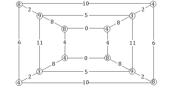
These edge-coloring properties are what we wish to preserve with our definition of strong \(\Gamma\)-zonal and \(\Gamma\)-cozonal labelings. Let \(G\) be a \(2\)-connected plane graph. We will say that an edge coloring \(f:E(G)\rightarrow \Gamma\) is proper vertex cyclic if for each \(v\in V(G)\) no two edges incident with \(v\) have the same color, and the difference between two consecutive edge colors about \(v\) is constant on \(v\). Specifically, \(f\) is a proper vertex cyclic edge coloring if \(f\) is proper and there is a well-defined function \(f':V(G)\rightarrow \Gamma\setminus \{0\}\) such that for any edge \(e\) incident with \(v\) and the consecutive counterclockwise edge \(e'\), \(f(e')-f(e)=f'(v)\). Similarly, an edge coloring \(g:E(G)\rightarrow \Gamma\) is proper region cyclic if for each \(R\in F(G)\) no two edges on the boundary of \(R\) have the same color, and the difference between two consecutive edge colors on the boundary of \(R\) is constant on \(R\). An example of a proper vertex cyclic edge coloring will be given in Figure 8. It is worth noting that when \(\Gamma\simeq \mathbb{Z}_3\), proper edge 3-colorings and tricolorings necessarily have this cyclic property.
We will now prove the motivating property behind strong \(\Gamma\)-cozonal, and therefore strong \(\Gamma\)-zonal, labelings. This will closely follow the approach used to prove Theorem 1.4 in [2], except that some properties will be generalized. To begin we will require some additional definitions.
The following definitions are adapted from those introduced in [2]. Let \(G\) be a \(2\)-connected plane graph with \(\Gamma\)-cozonal labeling \(\ell^*\). Let \(v\in V(G)\) with ordered pair of edges \((e,e')\) incident with \(v\) such that a subset of consecutive edges incident with \(v\) are given by \(e=e_0, e_1, …, e_k=e'\) in clockwise order. Denote the region between the edges \(e_i, e_{i+1}\) in the clockwise direction as \(R_i\), noting that \(R_i\ne R_j\) for \(i\ne j\). The zangle \(\angle(e,e')\) about \(v\) between the ordered pair of edges \((e,e')\) is defined as the sum \(\sum\limits_{i=0}^{k-1}\ell^*(R_i)\). This sums the region labels between the two edges in the clockwise direction. We say that \(\angle(e,e)=0\), as the sum is equivalently either \(0\) as the empty sum, or \(0\) as the sum of all regions incident with \(v\) in a cozonal labeling. An example is given in Figure 4.
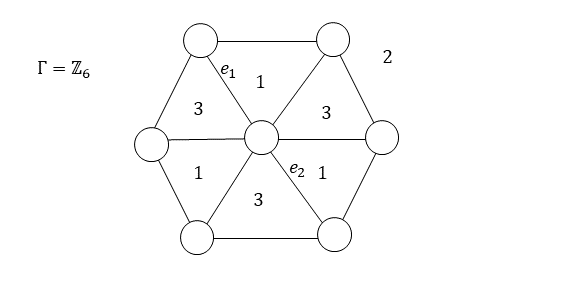
Next, an inner \(\Gamma\)-cozonal labeling is a labeling \(\ell^*:F(G)\rightarrow \Gamma\) such that exactly one region \(R\) (embedded as the exterior region) has the label \(0\), and for all vertices \(v\) not on the boundary of \(R\), \(\ell^*(v)=0.\) We ignore the exterior region when determining whether an inner \(\Gamma\)-cozonal labeling is strong. Let the exterior region be bounded by the cycle \(C_R=(v_0, e_0, v_1,…, e_{n-1}, v_n=v_0)\) with vertices and edges in counterclockwise order (with respect to a point interior to the cycle). We define the zangle \(\angle(e_{i}, e_{i-1})\) containing \(R\) to be \(-\angle(e_{i-1}, e_i)=-\ell^*(v_i),\) and calculate any other zangle centered at \(v_i\) and containing \(R\) as the sum of smaller consecutive zangles. An example is given in Figure 5.
The following propositions appear in [2].
Proposition 4.1. Let \(G\) be a plane triangulation or inner triangulation, let \(B\) be the boundary of the exterior region, and let \(\ell^*\) be an inner \(\mathbb{Z}_3\)-cozonal labeling of \(G\). Then \[\sum\limits_{v\in V(B)}\ell^*(v)=0.\]
Proposition 4.2. Let \(G\) be a \(2\)-connected plane triangulation or inner triangulation, let \(G\) have a \(\mathbb{Z}_3\)-cozonal or inner \(\mathbb{Z}_3\)-cozonal labeling \(\ell^*\), and let \(e, e'\in E(G).\) Let \(W_1, W_2\) be two walks \((u_0,e_0=e, u_1, …,e_{n-1}=e', u_n)\) and \((v_0,f_0=e,v_1,…,f_{m-1}=e', v_m)\). Then \[\sum\limits_{i=1}^{n-1}\angle(e_{i-1}, e_i)=\sum\limits_{i=1}^{m-1}\angle(f_{i-1},f_i).\]
We generalize these both here.
Lemma 4.3. Let \(G\) be a \(2\)-connected plane graph, let \(B\) be the boundary of the exterior region, and let \(\ell^*\) be a strong inner \(\Gamma\)-cozonal labeling of \(G\). Then \[\sum\limits_{v\in V(B)}\ell^*(v)=0.\]
Proof. Consider \(\sum\limits_{v\in V(G)}\ell^*(v)\). Since \(\ell^*(v)\) is the sum of all region labels incident with \(v\), this sums each region label once for each vertex on its boundary. Let \(B_R\) denote the boundary of the region \(R\). Then, \[\sum\limits_{v\in V(G)}\ell^*(v)=\sum\limits_{R \in F(G)}\left(\sum\limits_{v\in V(B_R)}\ell^*(R)\right)=\sum\limits_{R\in F(G)}|V(B_{R})|\ell^*(R).\]
Since the exterior region has a label of \(0\), we can ignore the exterior region. For all other regions, \(\ell^*(R)\) has additive order \(|V(B_{R})|\), and thus this sum is \(0\). However, we also know that \(\ell^*(v)=0\) for all vertices not in \(V(B)\). Therefore, it must be that \(\sum\limits_{v\in V(B)}\ell^*(v)=0\). ◻
Lemma 4.4. Let \(G\) be a \(2\)-connected plane graph, let \(G\) have a strong \(\Gamma\)-cozonal or inner \(\Gamma\)-cozonal labeling \(\ell^*\), and let \(e, e'\in E(G)\). Let \(W_1, W_2\) be two walks \((u_0,e_0=e, u_1, …,e_{n-1}=e', u_n)\) and \((v_0,f_0=e,v_1,…,f_{m-1}=e', v_m)\). Then \[\sum\limits_{i=1}^{n-1}\angle(e_{i-1}, e_i)=\sum\limits_{i=1}^{m-1}\angle(f_{i-1},f_i).\]
We will omit a full proof of Lemma 4.4 here, as the (somewhat lengthy) proof is identical to that in [2] for Proposition 4.2. To summarize the proof of Lemma 4.4, we begin by using Lemma 4.3 to show that for any cycle \(C\) in \(G\), the zangles interior to the cycle between consecutive cycle edges sum to \(0\). This is also true for the zangles exterior to the cycle. This result is then extended to the sum of zangles between consecutive edges in a closed walk (including the zangle between the first and last edge) using properties of zangles. Lemma 4.4 is then proven by concatenating \(W_1\) and the reverse of \(W_2\) into a closed walk and using this extended result. The only reason why Proposition 4.2 is restricted to plane triangulations and inner triangulations is to ensure that Proposition 4.1 holds. Given that Lemma 4.3 generalizes Proposition 4.1, it follows that Lemma 4.4 is the generalization of Proposition 4.2.
As a result of Lemma 4.4, given any two edges \(e_1, e_2\in E(G),\) the sum of zangles between consecutive edges on any walk starting with \(e_1\) and ending with \(e_2\) is equivalent, and we can define this value as the \(\Gamma\)-cozonal difference \(\mathop{\mathrm{coz_\Gamma}}(e_2-e_1)\). By concatenating a walk from \(e_1\) to \(e_2\) ending with \(uv\) with a walk from \(e_2\) to \(e_3\) beginning with \(vu\), we see that \(\mathop{\mathrm{coz_\Gamma}}(e_2-e_1)+\mathop{\mathrm{coz_\Gamma}}(e_3-e_2)=\mathop{\mathrm{coz_\Gamma}}(e_3-e_1).\) We can now prove our motivating theorem.
Theorem 4.5. Let \(G\) be \(2\)-connected, and let \(\Gamma\) be an abelian group. Then there exists a proper vertex cyclic edge coloring \(f:E(G)\rightarrow \Gamma\) if and only if \(G\) admits a strong \(\Gamma\)-zonal labeling. Dually, there exists a proper region cyclic edge coloring \(g:E(G) \rightarrow \Gamma\) if and only if \(G\) admits a strong \(\Gamma\)-cozonal labeling.
Proof. We will prove this from the \(\Gamma\)-cozonal perspective. First, let \(\ell^*:F(G)\rightarrow \Gamma\setminus \{0\}\) be a strong \(\Gamma\)-cozonal labeling, and choose an edge \(e' \in E(G).\) Let \(g:E(G)\rightarrow \Gamma\) be given by \(g(e)=\mathop{\mathrm{coz_\Gamma}}(e-e')\). Now consider a region \(R\in F(G)\), and let the edges on the boundary of \(R\) be given in counterclockwise order \((e_0, e_1, …, e_{k-1}, e_0)\) with subscripts in \(\mathbb{Z}_k\). Consider edges \(e_i, e_j\). Then \(g(e_j)-g(e_i)=\mathop{\mathrm{coz_\Gamma}}(e_j-e')-\mathop{\mathrm{coz_\Gamma}}(e_i-e')=\mathop{\mathrm{coz_\Gamma}}(e_j-e_i)\). This \(\Gamma\)-cozonal difference can be given by the path along the boundary of \(R\), which can be calculated by adding the label \(\ell^*(R)\) a total of \((j-i)\) times. This is illustrated in Figure 6. This therefore implies both that the difference between two consecutive colors is equal to \(\ell^*(R)\) and therefore constant on \(R\), and that for \(i\not \equiv j \pmod k\), \(g(e_i)\ne g(e_j)\). Thus, \(g\) is a proper region cyclic edge coloring of \(G\).
Now, let \(g:E(G)\rightarrow \Gamma\) be a proper region cyclic edge coloring of \(G\), and let \(\ell^*:F(G)\rightarrow \Gamma\setminus \{0\}\) be given by the constant difference \(\ell^*(R)=g(e'')-g(e')\) for two consecutive counterclockwise edges \(e', e''\) along the boundary \(B_R\) of \(R\). We see that since \(g\) is proper, \(j\ell^*(R) \ne 0\) for \(j < |V(B_R)|.\) In addition, after going about the boundary of \(R\) once we must return to the original color. Therefore, it follows that \(|V(B_R)|\ell^*(R)=0\), and the additive order of \(\ell^*(R)\) is given by \(|V(B_R)|.\)
Next, consider a vertex \(v\in V(G),\) let the edges incident with \(v\) be given by \(e_0, e_1,…, e_{k-1}\) in clockwise order with subscripts in \(\mathbb{Z}_k\), and let \(R_i\) be the region between edges \(e_i, e_{i+1}\) in the clockwise direction. Then \(\ell^*(v)=\sum\limits_{i=0}^{k-1}\ell^*(R_i)\). However, the edges \(e_i, e_{i+1}\) are consecutive counterclockwise on the boundary of \(R_i\), and therefore \(\ell^*(R_i)=g(e_{i+1})-g(e_i).\) Therefore, \[\ell^*(v)=\sum\limits_{i=0}^{k-1}\ell^*(R_i)=\sum\limits_{i=0}^{k-1}(g(e_{i+1})-g(e_i))=\sum\limits_{i=0}^{k-1}g(e_{i+1})-\sum\limits_{i=0}^{k-1}g(e_i).\]
Clearly \(\sum\limits_{i=0}^{k-1}g(e_{i+1})=\sum\limits_{i=0}^{k-1}g(e_i),\) and therefore \(\ell^*\) is \(\Gamma\)-cozonal. Since the additive order of \(\ell^*(R)\) is equal to \(|V(B_R)|\) for all \(R\in F(G)\), this is a strong \(\Gamma\)-cozonal labeling. ◻
It is generally much harder to find strong \(\Gamma\)-zonal and \(\Gamma\)-cozonal labelings of plane graphs. However, there are some observations that follow easily from our previous results.
Observation 4.6. Let \(C_n\) be a cycle with \(n\ge 3\), and let \(\Gamma\) be an abelian group with an element \(g\) of order \(n\). Then the labeling \(\ell^*:F(C_n)\rightarrow \Gamma\setminus \{0\}\) assigning elements \(g\) and \(-g\) to the two regions of \(C_n\) is a strong \(\Gamma\)-cozonal labeling of \(C_n\).
Observation 4.7. Let \(C_n\) be a cycle with \(n\ge 3\), and let \(\Gamma\) be an abelian group with at least one element \(g\) of order \(2\) if \(n\) is even, or at least two distinct elements \(g, g'\) of order \(2\) if \(n\) is odd. Then \(C_n\) is strong \(\Gamma\)-zonal.
Now we consider wheels \(W_n\). Since \(W_3=K_4\), \(W_3\) is zonal and therefore strong \(\mathbb{Z}_3\)-zonal, and therefore strong \(\Gamma\)-zonal for any group \(\Gamma\) having at least one element of order \(3\). The case for \(n>3\) is very different.
Theorem 4.8. Let \(n>3.\) Then the wheel \(W_n\) does not have a strong \(\Gamma\)-zonal labeling for any abelian group \(\Gamma\).
Proof. Suppose there were a strong \(\Gamma\)-zonal labeling \(\ell:V(W_n)\rightarrow \Gamma\setminus \{0\}\) for some group \(\Gamma\). Consider a triangular region \(R\) of \(W_n\). Such a region has two vertices \(v_1, v_2\) of degree \(3\) and one vertex \(u\) of degree \(n>3\) on its boundary. Then, \(3\ell(R)=3(\ell(v_1)+\ell(v_2)+\ell(u))=0+0+3\ell(u)\ne 0.\) Since \(3\ell(R)\ne 0,\) clearly \(\ell(R)\ne 0,\) and there cannot be a strong \(\Gamma\)-zonal labeling of \(W_n.\) ◻
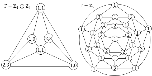
Not only is the wheel an example of a \(3\)-connected simple plane graph, but all \(3\)-connected plane graphs are simple. To verify this claim, suppose we have a plane graph that has parallel edges between vertices \(u\) and \(v\). Then the vertices \(u\) and \(v\) form a vertex cut. Thus, \(3\)-connected plane graphs are necessarily simple. Such graphs are interesting due not only to their high connectivity, but because the dual \(G^*\) of a \(3\)-connected plane graph \(G\) is also a \(3\)-connected plane graph, and therefore both graphs are simple. Now, we already know that all \(3\)-connected cubic plane graphs are strong \(\mathbb{Z}_3\)-zonal. We demonstrate two additional \(3\)-connected plane graphs which are strong \(\mathbb{Z}_4\oplus\mathbb{Z}_4\)– and \(\mathbb{Z}_5\)– zonal in Figure 7.
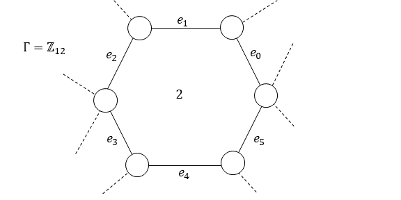
While all of our examples thus far of strong \(\Gamma\)-zonal labelings have been of regular graphs, this need not be the case. In Figure 8 we exhibit a \(\mathbb{Z}_{12}\)-zonal labeling of a generalized prism, as well as the induced proper vertex cyclic edge \(\mathbb{Z}_{12}\)-coloring.
One may wonder why the group \(\mathbb{Z}_4\oplus\mathbb{Z}_4\) was chosen for the example in Figure 7, instead of the simpler \(\mathbb{Z}_4\). This is due to a surprising result on \(3\)-connected plane graphs.
Theorem 4.9. Let \(G\) be a \(3\)-connected plane graph having no vertices of degree \(3\) or \(5\), and let \(G\) be strong \(\Gamma\)-zonal for some abelian group \(\Gamma\). Then \(\Gamma\) must contain a subgroup isomorphic to \(\mathbb{Z}_4\oplus \mathbb{Z}_4\).
Proof. Assume by way of contradiction that \(G\) has a strong \(\Gamma\)-zonal labeling \(\ell\) such that \(\Gamma\) does not have a subgroup isomorphic to \(\mathbb{Z}_4\oplus \mathbb{Z}_4\). Since the largest minimum degree of a plane graph is \(5\) and \(G\) is \(3\)-connected, \(G\) must have at least one vertex of degree \(4\). Let \(n=|V(G)|, m=|E(G)|,\) let \(r_3\) be the number of triangular regions, and let \(r_4\) be the number of regions having at least \(4\) vertices on their boundary. By the Euler identity, we have that \(n-m+r_3+r_4=2,\) and therefore \(4n-4m+4r_3+4r_4=8.\) Furthermore, since each edge appears on the boundary of two regions, we have that \(2m \ge 3r_3+4r_4.\) Therefore, \[\begin{split} 8&=4n-4m+4r_3+4r_4 \\ &\le 4n-2m+r_3 \\ &=\sum\limits_{v\in V(G)}(4-\deg(v))+r_3. \end{split}\]
We would first like to prove that if \(\ell\) is strong \(\Gamma\)-zonal, then each triangle of \(G\) must have on its boundary either no vertices of degree \(4\); have vertices with degrees \(4, 6,\) and at least \(12\); have vertices with degrees \(4, 7,\) and at least \(14\); or otherwise have one vertex of degree \(4\) and at least two vertices of degree at least \(8\).
Case 1. \(T\) has three vertices of degree \(4\) on its boundary.
Consider the labeling \(2\ell:F(G)\rightarrow 2\Gamma\). Since no vertex has degree \(2\), no vertex has a label with additive order \(2\) under \(\ell\), and thus \(2\ell\) is a \(2\Gamma\)-zonal labeling assigning each vertex of degree \(4\) a label with additive order \(2\). Suppose that there are two distinct elements \(2g_1, 2g_2\in 2\Gamma\) with additive order \(2\). Then \(2g_2-2g_1\) also has additive order \(2\) in \(2\Gamma,\) and \(g_1, g_2, g_2-g_1\) each have additive order \(4\) in \(\Gamma\). By considering all abeliean groups generated by two elements of order \(4\) (that is, \(\mathbb{Z}_4, \mathbb{Z}_4\oplus \mathbb{Z}_2, \mathbb{Z}_4\oplus \mathbb{Z}_4\)), we see that the only group with two order \(4\) elements whose difference is also order \(4\) is \(\mathbb{Z}_4\oplus \mathbb{Z}_4\). Thus, \(g_1\) and \(g_2\) generate a subgroup isomorphic to \(\mathbb{Z}_4\oplus \mathbb{Z}_4\). Since \(\mathbb{Z}_4\oplus \mathbb{Z}_4\) is not isomorphic to a subgroup of \(\Gamma\), it follows that \(2\Gamma\) must have exactly one element \(g\) of order \(2\), and therefore \(2\ell(T)=3g\ne 0.\) Therefore, \(T\) cannot have three vertices of degree \(4\) on its boundary.
Case 2. \(T\) has two vertices of degree \(4\) on its boundary.
Next, assume \(R\) has exactly two vertices \(v_1, v_2\) of degree \(4\) on its boundary and a third vertex \(v_3.\) Then \(4\ell(T)=4(\ell(v_1)+\ell(v_2)+\ell(v_3))=0+0+4\ell(v_3)\ne 0.\) Therefore, we see that \(R\) has at most one vertex of degree \(4\) on its boundary.
Case 3. \(T\) has one vertex of degree \(4\) on its boundary.
Subcase 3.1. \(T\) also has a vertex of degree \(6\) on its boundary.
Let \(v_1\) have degree \(4\) and \(v_2\) have degree \(6\). If the third vertex \(v_3\) also has degree \(6\), then \(6\ell(T)=6\ell(v_1)+0+0\ne 0\). Otherwise if \(v_3\) has degree less than \(12\), then the degree is not a divisor of \(12\), and \(12\ell(T)=0+0+12\ell(v_3)\ne 0.\) Therefore if two vertices have degrees \(4, 6\), the third must have degree at least \(12\).
Subcase 3.2. \(T\) also has a vertex of degree \(7\) on its boundary.
Let \(v_1\) have degree \(4\) and let \(v_2\) have degree \(7\). If the third vertex \(v_3\) has degree \(7\), then \(7\ell(R)=7\ell(v_1)+0+0\ne 0\). If \(v_3\) otherwise has degree less than \(14\), then the degree is not a divisor of \(28\), and \(28\ell(R)=0+0+28\ell(v_3)\ne 0.\) Therefore if two vertices have degrees \(4\), \(7\), the third must have degree at least \(14\).
Subcase 3.3. Both other vertices on the boundary of \(T\) have degree at least \(8\).
This does not contradict the strong \(\Gamma\)-zonality of \(G\).
Case 4. \(T\) does not have any vertices of degree \(4\) on its boundary.
This also does not contradict the strong \(\Gamma\)-zonality of \(G\).
Thus, we have shown that if \(G\) is strong \(\Gamma\)-zonal for some \(\Gamma\) not containing a subgroup isomorphic to \(\mathbb{Z}_4\oplus \mathbb{Z}_4\), then each triangle has one of the previously described configurations.
We will now proceed by discharging. Assign to each triangle a charge of \(1\), and assign to each vertex the charge \(4-\deg(v).\) The total of all charges is therefore at least \(8\). We redistribute charges from each triangle \(T\) as follows: First, if \(T\) has no vertices of degree \(4\) on its boundary, then we transfer \(1/3\) of its charge to each vertex on its boundary. Otherwise, if \(T\) has a vertex of degree \(4\) and a vertex of degree \(6\) or \(7\) on its boundary, we transfer \(1/3\) charge to the vertex of degree \(6\) or \(7\) and \(2/3\) charge to the vertex having degree at least \(12\). Lastly, if \(T\) has a vertex of degree \(4\) and two vertices having degree at least \(8\), we redistribute \(1/2\) charge to each vertex of degree at least \(8\). In this way the total charge is still at least \(8\), but each triangle has a charge of \(0\).
Now consider the charges of the vertices. Each vertex of degree \(4\) started with \(0\) charge and gained no additional charge. Each vertex of degree \(6\) or \(7\) received at most \(1/3\) charge from each incident region, resulting in a final charge of at most \(4-\deg(v)+\deg(v)/3\le 0.\) Each vertex of degree between \(8\) and \(11\) received at most \(1/2\) charge from each incident region, resulting in a final charge of at most \(4-\deg(v)+\deg(v)/2\le 0\). Finally, each vertex of degree \(12\) or higher received at most \(2/3\) charge from each incident region, resulting in a final charge of at most \(4-\deg(v)+2\deg(v)/3\le 0.\) Therefore, no vertex or region has a positive charge, contradicting the fact that the total charges sum to at least \(8\). Therefore, it is impossible for every triangle to have one of the desired configurations, and \(\ell\) cannot be a strong \(\Gamma\)-zonal labeling. This is a contradiction, and therefore \(\Gamma\) must have a subgroup isomorphic to \(\mathbb{Z}_4\oplus \mathbb{Z}_4.\) ◻
We have seen that \(K_4\) is strong \(\mathbb{Z}_3\)-zonal, the octahedron is strong \(\mathbb{Z}_4\oplus \mathbb{Z}_4\)-zonal, and there exists a \(3\)-connected plane graph which is strong \(\mathbb{Z}_5\)-zonal. We call this strong \(\mathbb{Z}_5\)-zonal graph \(G_5\). This allows us to completely characterize which groups can admit strong \(\Gamma\)-zonal labelings of \(3\)-connected plane graphs.
Theorem 4.10. Let \(\Gamma\) be an abelian group. Then there exists a \(3\)-connected plane graph \(G\) which is strong \(\Gamma\)-zonal if and only if \(\Gamma\) contains a subgroup isomorphic to either \(\mathbb{Z}_3, \mathbb{Z}_4\oplus \mathbb{Z}_4,\) or \(\mathbb{Z}_5\).
Proof. If \(\Gamma\) contains \(\mathbb{Z}_3, \mathbb{Z}_4\oplus \mathbb{Z}_4,\) or \(\mathbb{Z}_5\) as a subgroup, we have seen that there exists a \(3\)-connected plane graph (specifically \(K_4,\) the octahedron, or \(G_5\)) which is strong \(\Gamma\)-zonal, as we may restrict our labels to the appropriate subgroup.
Next, suppose that \(\Gamma\) does not contain \(\mathbb{Z}_3, \mathbb{Z}_4\oplus \mathbb{Z}_4,\) or \(\mathbb{Z}_5\) as a subgroup, and suppose that there exists a \(3\)-connected plane graph \(G\) which is \(\Gamma\)-zonal. Then \(\Gamma\) has no elements of additive order \(3, 5\), and therefore \(G\) does not have any vertices of degree \(3\) or \(5\). Since \(\Gamma\) also does not contain \(\mathbb{Z}_4\oplus \mathbb{Z}_4\) as a subgroup, by Theorem 4.9 \(G\) cannot be strong \(\Gamma\)-zonal. This is a contradiction, and no graph \(G\) can exist. ◻
Since the dual of a \(3\)-connected plane graph is also a \(3\)-connected plane graph, this dualizes as follows.
Corollary 4.11. Let \(\Gamma\) be an abelian group. Then there exists a \(3\)-connected plane graph \(G\) which is strong \(\Gamma\)-cozonal if and only if \(\Gamma\) contains a subgroup isomorphic to either \(\mathbb{Z}_3, \mathbb{Z}_4\oplus \mathbb{Z}_4,\) or \(\mathbb{Z}_5\).
There are several further areas of exploration in this topic. First, it may be of interest to find further families of graphs which are \(\Gamma\)-zonal and strong \(\Gamma\)-zonal, perhaps even in the context where \(G\) is not \(2\)-connected.
Next, note that we have fully characterized the groups \(\Gamma\) for which there exists a \(3\)-connected plane graph admitting a strong \(\Gamma\)-zonal labeling. We have not discussed labelings which are both strong and generative, and this leads to several much deeper questions:
Question 5.1. For which groups \(\Gamma\) does there exist a \(3\)-connected plane graph with a generative strong \(\Gamma\)-zonal labeling?
Question 5.2. For a given \(2\)-connected plane graph \(G\), for which abelian groups \(\Gamma\) does \(G\) admit a generative strong \(\Gamma\)-zonal labeling?
Combining our previous results on cycles, we see that the following are true:
Proposition 5.3. Let \(C_n\) be a cycle with \(n\ge 3\), and let \(\Gamma\) be an abelian group.
1. \(C_n\) is generative strong \(\Gamma\)-cozonal if and only if \(\Gamma\simeq \mathbb{Z}_n\).
2. \(C_n\) is generative strong \(\Gamma\)-zonal if and only if \(\Gamma\simeq \bigoplus_{i=1}^k\mathbb{Z}_2\) for some \(k\), where \(1\le k \le n-1\) if \(n\) is even, or \(2\le k \le n-1\) if \(n\) is odd.
Lastly, we could generalize to nonabelian groups (and change to multiplicative notation as appropriate), at least in the \(2\)-connected case where the boundary of each region is a cycle. As long as elements are multiplied in consecutive clockwise order, then elements multiplying to \(1\) will do so no matter which element is chosen as the starting element. To see this, note that if \(g_1g_2…g_k=1\), then \(g_1g_2…g_{i-1}\) and \(g_ig_{i+1}…g_{k-1}g_k\) are inverses for all \(i\) and commute; therefore \(g_ig_{i+1}…g_{k-1}g_kg_1g_2…g_{i-1}=1\) for any choice of \(i\). Thus the definitions of \(\Gamma\)-zonal, \(\Gamma\)-cozonal generalize, as well as their generative and strong extensions. However, the proof of Lemma 4.3 does not generalize, as this proof makes use of reordering and recombining terms. Therefore, a careful examination of the nonabelian case would be required in order to determine whether Theorem 4.5 generalizes.