
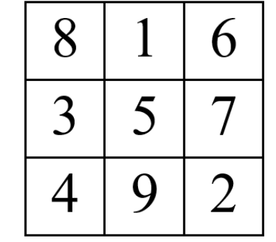
A magic square is a square grid containing a set of distinct numbers arranged in such a way that the sum of the numbers in any row, column, and main diagonals is always the same [2, 3]. The simplest magic square is the 3\(\mathrm{\times}\)3 square, where the nonrepetitive integers from 1 to 9 are arranged such that the sum of each row, column, and main diagonals equals 15 (Figure 1). The concept of magic squares dates back at least 4,000 years, with some of the earliest known examples being found in China [5].
Magic squares have fascinated mathematicians for centuries due to their seemingly endless combinations and patterns [4, 6, 7, 9, 13]. The number of possible magic squares for each arbitrary order increases significantly with each increase in order. For example, there is only one distinct 3\(\mathrm{\times}\)3 magic square using the first 9 integers. However, there are 880 distinct 4\(\mathrm{\times}\)4 magic squares using the first 16 integers, and an incredible 275,305,224 distinct 5\(\mathrm{\times}\)5 magic squares using the first 25 integers [14, 17]. The number of possible magic squares for orders seven and higher is far too large to be calculated precisely, and statistical estimations are the only feasible option [17]. These staggering numbers highlight the vast complexity and richness of magic squares, which continue to captivate and inspire mathematicians.
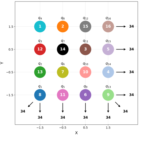
In recent years, there has been an increasing interest in using physics concepts to explore new patterns in magic squares [1, 8, 10, 12, 15, 16]. A novel way to analyze magic squares is to represent the numbers of the square with point masses [1, 12, 15] or electric charges [8, 10, 16] distributed regularly on a 2D lattice (Figure 2). This approach provides insights into the center of mass [1], moment of inertia [12] (inertia tensor [15]), electric multipoles [16], and electrostatic potential [8, 10] of magic squares. By applying the principles of physics to magic squares, researchers can gain a deeper understanding of the properties and characteristics of these intriguing mathematical objects that were previously undiscovered. For example, representing the integers of magic squares as magnitudes of electric charges on a two-dimensional lattice (Figure 2) enables the investigation of their electrostatic properties. New research has shown that the maximum and minimum electric potential values within 4\(\mathrm{\times}\)4 and 5\(\mathrm{\times}\)5 magic squares are only possible at specific grid points, following a distinct pattern [10]. Additionally, the sums of potentials along horizontal and vertical lines within the grid contain certain constants [10]. These findings suggest that the distribution of electrostatic potential in magic squares is not random but rather follows a striking pattern.
The aim of this paper is to explore an intriguing question: If one represents magic squares as a system of electric charges on a two-dimensional lattice and seeks to investigate their dynamics, the charges would quickly disperse due to Coulombic repulsion. Can a physical system be constructed to control the movement of these charges until they reach a quasi-static equilibrium? If so, do magic charges move along directions with symmetrical properties? Do they preserve their arrangement in order to maintain the magic sum? Will strong correlations emerge in the pairwise distances between charges after simulation? Furthermore, if the same analysis is applied to a random square containing the same integers but without satisfying the magic sum, will the results differ meaningfully from those of magic squares? Which configuration exhibits greater symmetry – magic squares or random squares?
Among the first experiments to levitate a single particle was Robert Millikan’s oil drop experiment, conducted in 1909. This is a classic example of how charged particles can be suspended using external forces. The experiment was designed to measure the fundamental charge of an electron. Millikan introduced tiny oil droplets into a chamber containing two parallel plates that generated an adjustable electric field. By fine-tuning this field, he counterbalanced the gravitational force acting on individual charged droplets, allowing them to remain suspended in equilibrium. Through careful analysis of the interplay between gravitational, viscous drag, and electrostatic forces, he demonstrated that electric charge is quantized.
Earnshaw’s theorem [11], named after Samuel Earnshaw, is a fundamental principle in electrostatics that states that a system of charges in static equilibrium cannot be maintained solely by electrostatic forces. In other words, it is impossible to trap a charged object in a stable equilibrium solely through electrostatic repulsion or attraction. This is because a configuration of charges that is stable in one dimension will necessarily be unstable in another dimension. The theorem applies to any system of point charges, regardless of the number of charges or their arrangement. Here, we introduce additional forces into the system of magic electric charges to counterbalance Coulombic repulsion and achieve quasi-static equilibrium, as described in detail in the Materials and Methods section.
We use the complete set of 4\(\mathrm{\times}\)4 magic squares (880 in total). Each row of the spreadsheet, magic_squares.xlsx (supplementary material), contains the numbers 1,…,16 arranged so that all row, column, and main diagonals sums equal 34. For a given row \(s\in \left\{1,\dots ,880\right\}\) we form a charge vector \({\boldsymbol{\mathrm{q}}}^{\left(s\right)}=\left(q^{\left(s\right)}_1,\dots ,q^{\left(s\right)}_{16}\right)\) by reading the 4\(\mathrm{\times}\)4 array row-major (left-to-right within rows, top-to-bottom across rows). These 16 integers are used as the electric charges. The 16 particles are initially placed at the 4\(\mathrm{\times}\)4 grid \(A=\left\{-1.5,\ -0.5,\ 0.5,\ 1.5\right\}\times \left\{-1.5,\ -0.5,\ 0.5,\ 1.5\right\}\subset {\mathbb{R}}^2\) as shown in Figure 2. Let \({\boldsymbol{\mathrm{r}}}_{0,i}=\left(x_{0,i}\ ,\ y_{0,i}\right)\) be the fixed reference point of particle \(i\). Initial conditions are: \({\boldsymbol{\mathrm{r}}}_i\left(0\right)={\boldsymbol{\mathrm{r}}}_{0,i}\) and \({\dot{\boldsymbol{\mathrm{r}}}}_i\left(0\right)=0\) where \({\dot{\boldsymbol{\mathrm{r}}}}_i\) represents the velocity of particle \(i\). Motion takes place in the full plane \({\mathbb{R}}^2\) with no boundaries.
We evolve 16 particles, carrying electric charges, governed by Coulomb-type pairwise repulsion, linear viscous damping, and linear “pinning” towards their reference points.
For particle \(i\) with mass \(m_i\) and electric charge \(q_i\), moving in \({\mathbb{R}}^2\), we assume it is (1) driven by the electric field \({\boldsymbol{\mathrm{E}}}_i\) generated by the other charges, (2) pulled toward its home point \({\boldsymbol{\mathrm{r}}}_{0,i}\) by a local harmonic potential with force constant \(k_i\), and (3) subject to linear viscous drag with coefficient \({\gamma }_i\). The position of particle \(i\) at time \(t\) is denoted by \({\boldsymbol{\mathrm{r}}}_i\left(t\right)\in {\mathbb{R}}^2\), its velocity by \({\dot{\boldsymbol{\mathrm{r}}}}_i\left(t\right)\), and its acceleration by \({\ddot{\boldsymbol{\mathrm{r}}}}_i\left(t\right)\). The force balance is represented by the equation: \[\label{GrindEQ__1_} m_i{\ddot{\boldsymbol{\mathrm{r}}}}_i\left(t\right)=q_i{\boldsymbol{\mathrm{E}}}_i\left(\left\{\boldsymbol{\mathrm{r}}\left(t\right)\right\}\right)-k_i\left({\boldsymbol{\mathrm{r}}}_i\left(t\right)-{\boldsymbol{\mathrm{r}}}_{0,i}\right)-{\gamma }_i{\dot{\boldsymbol{\mathrm{r}}}}_i\left(t\right), \tag{1}\] where \[\label{GrindEQ__2_} {\boldsymbol{\mathrm{E}}}_i\left(\left\{\boldsymbol{\mathrm{r}}\left(t\right)\right\}\right)=\sum_{j\neq i}{q_j\frac{{\boldsymbol{\mathrm{r}}}_i-{\boldsymbol{\mathrm{r}}}_j}{{\left({\left\|{\boldsymbol{\mathrm{r}}}_i-{\boldsymbol{\mathrm{r}}}_j\right\|}^2+\varepsilon \right)}^{3/2}},} \tag{2}\] with a small regularizer \(\varepsilon ={10}^{-9}\) included to avoid division by zero when two particles come very close.
We interpret \(q_i\in \left\{1,\dots ,16\right\}\) as a multiplicity: values \(q_i>1\) represent \(q_i\) identical charge copies that move rigidly together at site \(i\). Under this interpretation it is natural to take \(m_i=m_0q_i\), \({\gamma }_i={\gamma }_0q_i\), and \(k_i=k_0q_i\). Below we explain why each scaling is meaningful.
If site \(i\) contains \(q_i\) identical charge copies that move together, masses add: \(m_i=\underbrace{m_0+\dots +m_0}_{q_i\ \mathrm{times}}=m_0q_i\).
In the linear (small-speed) regime, each identical charge copy contributes a drag force \(-{\gamma }_0{\dot{\boldsymbol{\mathrm{r}}}}_i\). With \(q_i\) such copies moving together, these forces add: \[\label{GrindEQ__3_} {\boldsymbol{\mathrm{F}}}_{\mathrm{drag,}i}=-\sum^{q_i}_{c=1}{{\gamma }_0{\dot{\boldsymbol{\mathrm{r}}}}_i}=-\left({\gamma }_0q_i\right){\dot{\boldsymbol{\mathrm{r}}}}_i , \tag{3}\] hence \({\gamma }_i={\gamma }_0q_i\). Intuitively: more of the same material \(\mathrm{\Rightarrow }\) more independent linear dissipative channels, so the effective drag constant scales with \(q_i\).
We model the pinning by a fixed external potential well \(\mathrm{\Phi }\left(\mathrm{r}\right)\) (e.g. electrostatic or optical). The pinning force on particle \(i\) is \[\label{GrindEQ__4_} {\boldsymbol{\mathrm{F}}}_{\mathrm{pin,}i}=-q_i\mathrm{\nabla }\mathrm{\Phi }\left({\boldsymbol{\mathrm{r}}}_{\boldsymbol{i}}\right). \tag{4}\]
Let \({\boldsymbol{\mathrm{r}}}_{0,i}\) be a stable equilibrium (“home point”), so \(\mathrm{\nabla }\mathrm{\Phi }\left({\boldsymbol{\mathrm{r}}}_{0,i}\right)=0\). For small displacements, \({\boldsymbol{\mathrm{r}}}_i-{\boldsymbol{\mathrm{r}}}_{0,i}\), a first order Taylor expansion of the gradient gives \[\label{GrindEQ__5_} \mathrm{\nabla }\mathrm{\Phi }\left({\boldsymbol{\mathrm{r}}}_{\boldsymbol{i}}\right)\approx \underbrace{{\mathrm{\nabla }}^2\mathrm{\Phi }\left({\boldsymbol{\mathrm{r}}}_{0,i}\right)}_{\mathrm{Hessian}\ H}\left({\boldsymbol{\mathrm{r}}}_i-{\boldsymbol{\mathrm{r}}}_{0,i}\right), \tag{5}\] hence \[\label{GrindEQ__6_} {\boldsymbol{\mathrm{F}}}_{\mathrm{pin,}i}\approx -q_iH\left({\boldsymbol{\mathrm{r}}}_i-{\boldsymbol{\mathrm{r}}}_{0,i}\right). \tag{6}\]
In the isotropic case, \(H=\kappa I_3\), with \(I_3\) the 3\(\mathrm{\times}\)3 identity matrix. Comparing \({\boldsymbol{\mathrm{F}}}_{\mathrm{pin,}i}\) (Eq. (6)) with the local harmonic form ( Eq. (1), \(-k_i\left({\boldsymbol{\mathrm{r}}}_i\left(t\right)-{\boldsymbol{\mathrm{r}}}_{0,i}\right)\) ) shows that \(k_i=q_i\kappa =k_0q_i\), where \(k_0:= \kappa\) is the constant curvature of the potential well at \({\boldsymbol{\mathrm{r}}}_{0,i}\). Thus, under these conditions, the effective stiffness is proportional to the charge \(q_i\).
Inserting the charge-weighted parameters, \(m_i=m_0q_i\), \({\gamma }_i={\gamma }_0q_i\), and \(k_i=k_0q_i\) into Eq. (1) and then dividing by \(q_i\) yields the implemented form \[\label{GrindEQ__7_} m_0\ddot{{\boldsymbol{\mathrm{r}}}_i}\left(t\right)={\boldsymbol{\mathrm{E}}}_i\left(\left\{\boldsymbol{\mathrm{r}}\left(t\right)\right\}\right)-k_0\left({\boldsymbol{\mathrm{r}}}_i\left(t\right)-{\boldsymbol{\mathrm{r}}}_{0,i}\right)-{\gamma }_0{\dot{\boldsymbol{\mathrm{r}}}}_i\left(t\right). \tag{7}\]
We use a standard velocity-Verlet (leap-frog) [18] scheme with fixed time step \(\Delta t=0.01\) for \(T=2500\) steps per case. At time \(t\) we first compute the electric field \({\boldsymbol{\mathrm{E}}}_i\left(\left\{\boldsymbol{\mathrm{r}}\left(t\right)\right\}\right)\) for all \(i\). We then apply the half-kick: \[\label{GrindEQ__8_} {\boldsymbol{\mathrm{v}}}_i\leftarrow {\boldsymbol{\mathrm{v}}}_i+\frac{1}{2}{\boldsymbol{\mathrm{a}}}_i\Delta t,\qquad {\boldsymbol{\mathrm{a}}}_i:= \frac{{\boldsymbol{\mathrm{E}}}_i-k_0\left({\boldsymbol{\mathrm{r}}}_i-{\boldsymbol{\mathrm{r}}}_{0,i}\right)-{\gamma }_0{\boldsymbol{\mathrm{v}}}_i}{m_0}. \tag{8}\]
Then, to stabilize the explicit scheme we cap the speed, \[\label{GrindEQ__9_} {\boldsymbol{\mathrm{v}}}_i\leftarrow \frac{{\boldsymbol{\mathrm{v}}}_i}{{\mathrm{max} \left\{1,\ \ \ \frac{\left\|{\boldsymbol{\mathrm{v}}}_i\right\|}{V_{\mathrm{max}}}\right\}\ }} ,\qquad V_{\mathrm{max}}=5, \tag{9}\] perform the drift \[\label{GrindEQ__10_} {\boldsymbol{\mathrm{r}}}_i\leftarrow {\boldsymbol{\mathrm{r}}}_i+{\boldsymbol{\mathrm{v}}}_i\Delta t, \tag{10}\] recompute \({\boldsymbol{\mathrm{E}}}_i\) at the updated positions, and apply the second half-kick \[\label{GrindEQ__11_} {\boldsymbol{\mathrm{v}}}_i\leftarrow {\boldsymbol{\mathrm{v}}}_i+\frac{1}{2}{\boldsymbol{\mathrm{a}}}^{\mathrm{new}}_i\Delta t, \tag{11}\] with \({\boldsymbol{\mathrm{a}}}^{\mathrm{new}}_i\) defined as Eq. (8) using the updated field and velocity.
We track how close the system is to settling using one simple number. At step \(t\), let \({\boldsymbol{\mathrm{v}}}_i\left(t\right)\) be the velocity of particle \(i\). We compute root-mean-square (RMS) speed \[\label{GrindEQ__12_} \mathrm{RMS}\left(\mathrm{t}\right)={\left(\frac{1}{16}\sum_i{{\left\|{\boldsymbol{\mathrm{v}}}_i\left(t\right)\right\|}^2}\right)}^{1/2}. \tag{12}\]
If the configuration has effectively stopped moving, \(\mathrm{RMS}\left(\mathrm{t}\right)\) is close to zero. This is our primary indicator of convergence.
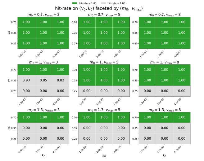
Numerical behavior can depend on modeling constants. To show our conclusions are not tied to a single choice, we repeat shorter runs over a small grid of parameter values \(\left(m_0,\ {\gamma }_0,k_0,V_{\mathrm{max}}\right)\) and record simple success/failure outcome. A run is declared a “hit” if the system clearly settles near a steady configuration. For each parameter setting we run the same procedure on a subset of 40 magic squares and compute the hit-rate: \[\label{GrindEQ__13_} \mathrm{hit\ rate=}\frac{\mathrm{number\ of\ cases\ that\ hit}}{40}. \tag{13}\]
This is simply the fraction of cases that settled under that setting. If the hit-rate stays high (or trends similarly) across the grid, then the observed behavior is robust and not an artifact of one particular parameter values. We summarize the results with heat maps of convergence success on the \(\left({\gamma }_0,\ k_0\right)\) plane, faceted by \(\left(m_0,\ V_{max}\right)\), to address straightforward questions such as, “Does increasing \(k_0\) generally help the system settle?”
We produce three primary figures (with a few minor diagnostics).
(1) Final-position map
For each case, we plot the equilibrium positions of all 16 particles. Colors encode particle index (1–16), not charge value. This lets us see at a glance whether indices are randomly dispersed or form clusters/regular patterns that reflect the symmetries of magic squares. For comparison, we generate 880 random 4\(\mathrm{\times}\)4 arrays (permutations of 1–16 that do not satisfy the magic-square constraints), simulate them in the same way, and place their final-position map side-by-side with the magic-square map.
(2) Displacement–correlation analysis
This analysis asks a simple question: when one pair of indices ends up far apart, does another pair tend to be far apart as well, across many squares? If “yes” happens more often for magic squares than for random ones, that’s evidence of coordinated spacing created by the magic-square structure.
For each Cartesian coordinate axis \(\mathrm{\Omega }\mathrm{\in }\left\{X,Y\right\}\) and each unordered index pair \(\left(a,b\right)\) with \(1\le a<b\le 16\), we define \[\label{GrindEQ__14_} D^{\left(\mathrm{\Omega }\right)}_{a,b}\left(s\right)=\left|{\mathrm{\Omega }}^{\left(s\right)}_a-{\mathrm{\Omega }}^{\left(s\right)}_b\right|,\ \ \ \ \ \ \ \ \ \ s=1,\dots ,880, \tag{14}\] where \({\mathrm{\Omega }}^{\left(s\right)}_i\) is the final \(x\ \left(\mathrm{or}\ y\right)\) coordinate of index \(i\) in case \(s\). For any two-displacement series \(D^{\left(\mathrm{\Omega }\right)}_{a,b}\) and \(D^{\left(\mathrm{\Omega }\right)}_{c,d}\), we compute the Pearson correlation coefficient \(r\) across cases. All such pair-of-pairs are ranked by \(\left|r\right|\) in the magic dataset, the same pair-of-pairs are then evaluated in the random dataset.
(3) Electrostatic potential at the geometric center
According to the literature, the electrostatic potential at the center of any 4\(\mathrm{\times}\)4 magic square has a unique value, independent of the specific distribution of magic numbers [8, 10]. This property arises from the symmetrical arrangement of integers within magic squares. In this study, we calculate the electrostatic potential at the center of both magic and random squares, before and after simulation, to examine how it changes. This allows us to clearly distinguish the behavior of magic squares from that of random ones.
Let \(q_i\in \left\{1,\dots ,16\right\}\) be the charges and \({\boldsymbol{\mathrm{r}}}_i=\left(x_i\ ,\ y_i\right)\in {\mathbb{R}}^2\) their positions for a given configuration. Define the geometric center \[\label{GrindEQ__15_} \mathrm{C}=\frac{1}{16}\sum^{16}_{i=1}{{\boldsymbol{\mathrm{r}}}_i} . \tag{15}\]
The regularized Coulomb potential at this center is \[\label{GrindEQ__16_} \mathrm{\Phi }\left(C\right)=\frac{1}{16}\sum^{16}_{i=1}{\frac{q_i}{\sqrt{{\left\|r_i-C\right\|}^2+\varepsilon }},\ \ \ \ \ \ \ \ \ \ \varepsilon ={10}^{-9}}. \tag{16}\]
(Here \(\left\|\right\|\) is the Euclidean norm; \(\varepsilon\) just prevents division by zero.)
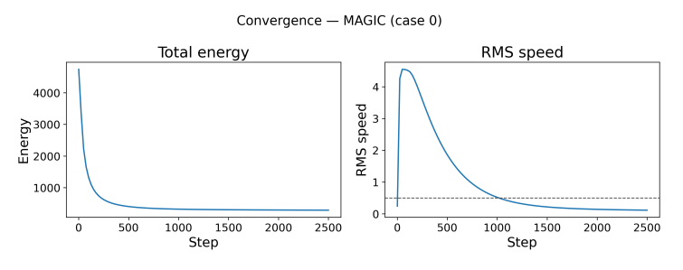
Figure 3 shows a representative magic case (index 0). The total energy (Coulomb + pinning) drops steeply during the first few hundred steps and then approaches a plateau, decreasing by well over an order of magnitude within the first \(\sim \ 400-500\) steps and then changes only slowly thereafter. The RMS speed exhibits a short transient peak (\(\sim \ 4.5\)) and then decays roughly exponentially, crossing the reporting threshold (dashed line at 0.5) near \(t\approx 1000\) and reaching \(\sim \ 0.2\) by the end of the run. This pattern – rapid early dissipation followed by slow drift – is typical across cases (not shown) and indicates that damping and pinning dominate after the initial Coulomb push. We therefore run a fixed 2500 steps for all cases to keep logging uniform. Qualitatively, the geometry changes little once the RMS speed drops below the threshold, which justifies using the “final” positions for the comparisons that follow.
Across all 880 magic squares, the final positions form sixteen tight, well-separated clouds arranged on an annulus (Figure 4A). Each cloud corresponds to a fixed particle index (color); the same index repeatedly finishes in nearly the same radial/azimuthal sector across cases, without overlap between colors. For comparison, examine the colors and their order in Figure 4A relative to those in Figure 2. In contrast, the random ensemble produces broader, smeared arcs around the annulus and a discernible central accumulation (Figure 4B). Thus, although both ensembles “ringify” under Coulomb repulsion with pinning and damping, the magic ensemble converges to highly reproducible index-specific locations, while the random ensemble remains variable and less structured.
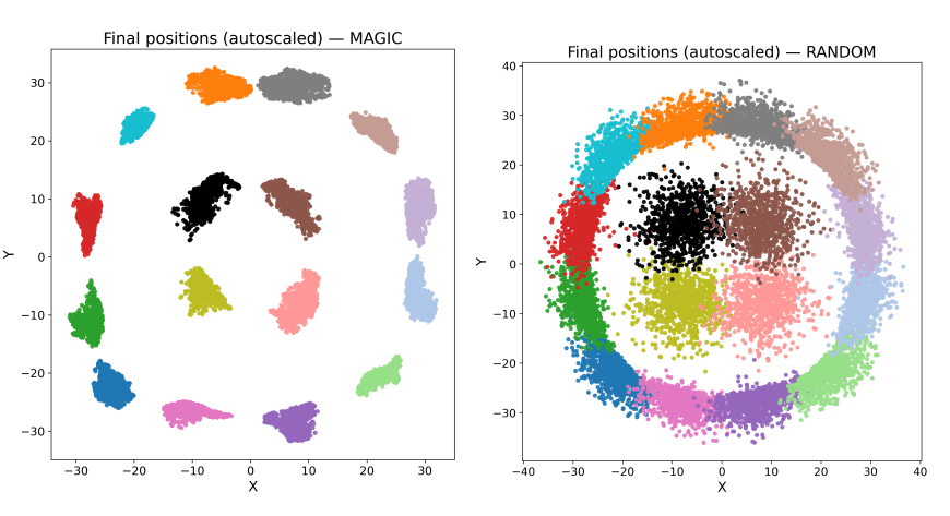
The magic constraint (balanced row/column/diagonal sums) imposes hidden symmetries that the dynamics preserve and amplify: particles labeled by index settle into consistent sectors over many independent runs. The random layouts lack those combinatorial symmetries and therefore do not exhibit the same deterministic mapping from index to sector.
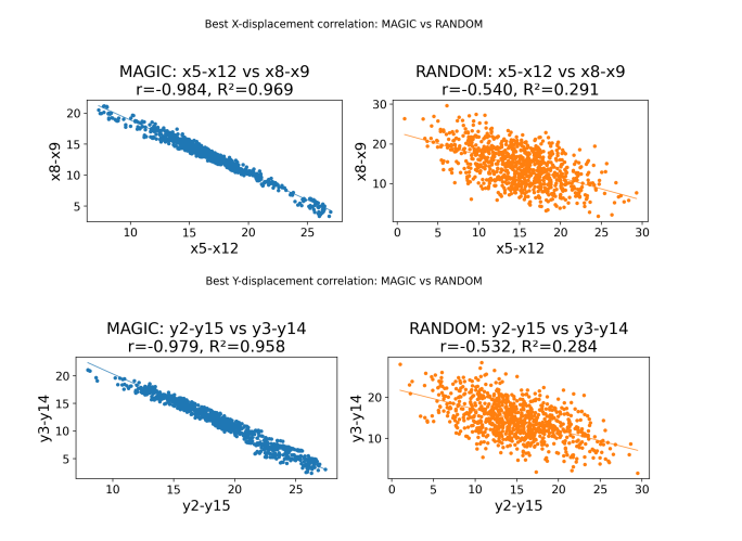
To quantify geometric regularity without relying on a single scalar (e.g., radius), we examined pairwise displacement series for each case: for every index pair \(\left(a,\ b\right)\) we built \(\left|x_a-x_b\right|\) and \(\left|y_a-y_b\right|\) across cases and then correlated these series between pairs of index-pairs (e.g. \(\left(x_a-x_b\right)\) vs \(\left(x_c-x_d\right)\) ).
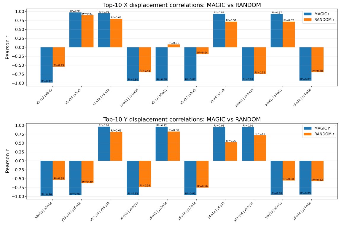
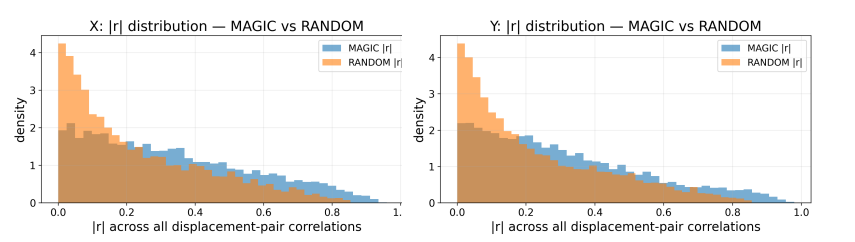
The best pair-of-pairs in the magic ensemble (\(\left(x_5-x_{12}\right)\) vs \(\left(x_8-x_9\right)\), and \(\left(y_2-y_{15}\right)\) vs \(\left(y_3-y_{14}\right)\); refer to Figure 2 to identify the locations to which these index pairs correspond.) produces near-perfect linear relationships in both axes (scatter panels are almost a line; Figure 5). For the same pair-of-pairs evaluated on the random ensemble the correlation is only moderate, with a visibly thicker cloud. This “best-case” gap is not an isolated phenomenon: when we take the top-10 pair-of-pairs (ranked by \(\left|r\right|\) in magic squares) and compare their correlations in Magic vs Random, the magic bars are consistently high while the random bars are consistently lower (Figure 6). Aggregating over all pair-of-pairs shows the same story: the \(\left|r\right|\) distribution for Magic is shifted toward stronger correlations (Figure 7A–B).
Correlation structure among displacement pairs is a sensitive probe of global organization. Magic squares induce rigid, reproducible dependencies (many pair-of-pairs are almost deterministically related), whereas random layouts produce only loose trends. The excess of high \(\left|r\right|\) and \(R^2\) in Magic is a global signature of that rigidity.
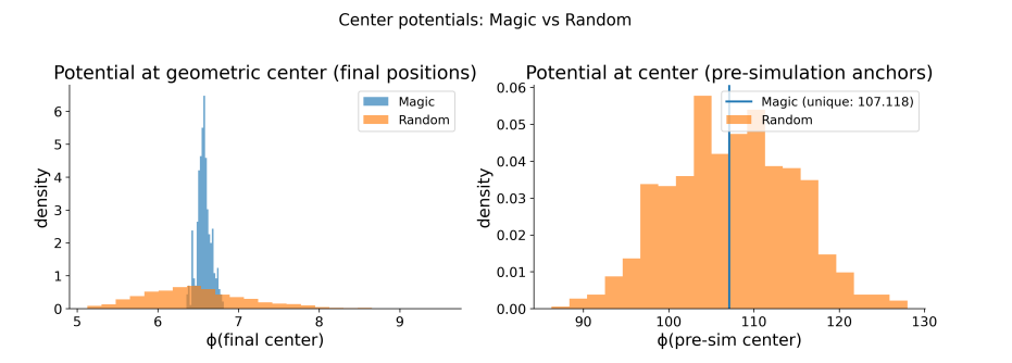
We also summarized each configuration by the Coulomb potential at its geometric center as described in Materials & Methods. Two comparisons are informative (Figure 8):
1. At the anchor center (pre-simulation): the magic ensemble collapses to a single value (vertical line), while the random ensemble is broad. This indicates an invariance of the magic layouts with respect to the center – empirically, magic squares distribute \(\{1,\dots,16\}\) over “distance classes” from the center in a way that yields an identical \(\sum_i{q_i/r_i}\) for all 880 cases.
2. At the final geometric center (post-simulation): the magic ensemble forms a narrow peak (very small variance), whereas the random ensemble remains substantially wider. Both ensembles “ringify,” so the means can be similar, but the variability is decisively smaller for magic cases – final states are much more reproducible.
The center potential acts as a stability/consistency marker rather than a strong separator of means. Magic squares exhibit (i) a pre-simulation invariance of the center potential and (ii) a post-simulation concentration to a tight band, both consistent with the highly structured clouds in Figure 4A.
A separate sensitivity sweep over 3\({}^{4}\) = 81 tuples (\(m_0\in \left\{0.7,\ 1,\ 1.3\right\},\\ {\gamma }_0\in \left\{0.25,\ 0.35,\ 0.7\right\},\ k_0\in \left\{0.001,\ 0.002,\ 0.004\right\},\ V_{\mathrm{max}}\in \left\{3,\ 5,\ 8\right\}\)) on a subset of 40 magic squares recorded a hit-rate per tuple (fraction of cases whose force-residual and RMS-speed fell below relaxed thresholds on a short streak). The output shows a median hit-rate of 1.00 and a mean of 0.662, indicating that many parameter settings (\(\mathrm{\sim}\) 63%) yield stable settling under the diagnostics (Figure 9). We used settings within this region (\(m_0=1,\ {\gamma }_0=0.35,\ k_0=0.002,\ V_{\mathrm{max}}=5\)) for the figures above, confirming that the qualitative findings are not tied to a single parameter choice.
We represent the integers in each 4\(\mathrm{\times}\)4 magic square as the magnitudes of 16 positive electric point charges placed at the grid’s anchor sites and then evolved under Coulomb repulsion, linear damping, and a pinning potential well toward those anchors. This work links a classical object of discrete mathematics – the 4\(\mathrm{\times}\)4 magic square – to a transparent continuous-time relaxation that exposes its hidden structure. Under Coulomb repulsion with linear damping and sitewise pinning, magic squares reliably evolve into sixteen compact, index-specific clusters on an annulus, whereas random permutations do not. A second, global view – correlations among inter-index displacements – confirms that magic squares encode strong, reproducible dependencies across many cases; in contrast, random squares exhibit only diffuse trends. A third summary – the center potential – distinguishes ensembles by reproducibility (narrow vs. broad distributions) rather than by means, again favoring magic squares. Together, these orthogonal readouts tell a coherent story: the magic constraint (equal row/column/diagonal sums) is not merely combinatorial; it generates robust geometric organization in a simple, physically interpretable flow.
Methodologically, the model is minimal, computationally light, and reproducible: charge-weighted parameters, a standard leapfrog integrator, and a small speed cap suffice. A focused sensitivity sweep demonstrates robust settling across a broad region of damping–stiffness pairs, so the qualitative findings do not depend on fine-tuning. The framework suggests several extensions: higher orders (5\(\mathrm{\times}\)5 and beyond), alternative or anisotropic pinning fields, stochastic forcing, or 3D embeddings; analytical work on the energy landscape and stationary configurations; and comparative studies across structured ensembles (e.g., associative, pandiagonal, and ultramagic magic squares) using the same correlation and potential readouts. More broadly, the approach offers a template for translating discrete balance conditions into macroscopic geometric signatures via quasi-static dynamics, opening a path to new diagnostics for symmetry, rigidity, and reproducibility in other combinatorial arrays.
The author wishes to thank the reviewer for their constructive comments, Professor Chérif F. Matta (Mount Saint Vincent University) for valuable discussions, and Nima Fahimi for his support.
All data and Python scripts are available from the corresponding author upon request.
There are no conflicts to declare.