
We assume that the reader has some familiarity with matroids and oriented matroids as in [1, 2]. Every orientation of a graphic matroid \(M(G)\) is realized by an orientation \(\tau\) of \(G\). Thus, up to reorientation \(M(G)\) has only one orientation (see, for example, [1, Propositions 7.9.3 and 7.9.4]).
Slilaty and Zaslavsky [4] characterized single-element extensions of graphic matroids in graphical terms using a struture called a cobiased graph. (Cobiased graphs will be reviewed in Seciton 2.) When \((G,\mathcal L)\) is a cobiased graph, the associated single-element extension of \(M(G)\) is denoted by \(J_0(G,\mathcal L)\). In this paper we will define an orientation of a cobiased graph \((G,\mathcal L)\) in terms of graphical structures. The orientation will be a pair \((o,\tau)\) in which: \(\tau\) is an orientation of the graph \(G\) and a \(o\) is a \(\{-1,0,+1\}\)-valued function which is defined using the bonds of \(G\) and is called pre-orientation. Our three main results are as follows. One, every orientation of \((G,\mathcal L)\), if one exists, produces an orientation of its matroid \(J_0(G,\mathcal L)\) (Theorem 4.2). Two, if \((o_1,\tau_1)\) and \((o_2,\tau_2)\) are orientations of \((G,\mathcal L)\) and \(G\) is 2-connected, then the associated orientations of \(J_0(G,\mathcal L)\) are equal by reorientation if and only if \(o_1=\pm o_2\) (Theorem 4.5). Three, any orientation of \(J_0(G,\mathcal L)\), if one exists, is given by some orientation \((o,\tau)\) of \((G,\mathcal L)\) (Theorem 4.7).
Single-element coextensions of graphic matroids were characterized by Zaslavsky [7, 8] and orientations of single-element coextensions of graphic matroids were characterized by Slilaty [3]. At first, it may appear that there is some kind of general duality relationship between co-biased graphs and biased graphs and thus between their respective matroids and thus between the orientations of cobiased graphs explained in this paper and those of biased graphs in [3]. This, however, is not the case because the class of graphic matroids is not closed under duality. If \(X\) is a single-element extension of graphic matroid \(M(G)\) by element \(e\) (i.e., \(X\backslash e=M(G)\)), then \(X^*\) is a single-element coextension of cographic matroid \(M^*(G)\) (i.e., \(M^*(G)=X^*/e\)). A foundational result of matroid theory is Whitney’s Theorem which states that \(M^*(G)=M(H)\) for some graph \(H\) if and only if \(G\) is planar. Therefore it is not the case that one can canonically view single-element extensions of graphic matroids as dual to single-element coextensions of graphic matroids. For this reason, the results of this paper are necessary in order to fully understand the structure of orientations of single-element extensions of graphic matroids.
Theorem 1.1(Whitney [6]). If \(M(G)\) is connected, then \(M^*(G)=M(H)\) if and only if \(H=G^*\) for some embedding of \(G\) in the plane (up to addition and removal of isolated vertices in \(H\)).
In the case that \(G\) is planar, however, there is a very natural duality between these two types of matroids and their orientations. We will explore this relationship in Section 5.
Let \(G\) be a graph and \(X\subset V(G)\). The coboundary of \(X\) is denoted by \(\delta(X)\) and is the set of non-loop edges of \(G\) with exactly one endpoint in \(X\). If \(G\backslash\delta(X)\) has exactly one more connected component that does \(G\), then \(\delta(X)\) is a bond in \(G\). Also, if \(B\) is a bond in \(G\) which separates a connected component of \(G\) into two connected subgraphs on vertex sets \(X\) and \(Y\), then we will also denote the bond \(B\) by \([X,Y]\). A subset \(X\subset V(G)\) for which \(\delta(X)\) is a bond of \(G\) is called bond boundary of \(B\). Thus every bond has exactly two boundaries. The pair \([X,Y]\) is considered to be unordered and so \(B=[X,Y]=[Y,X]=\delta(X)=\delta(Y)\).
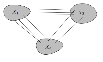
Consider a tripartition \(X_1,X_2,X_3\) of the vertices of one connected component of \(G\) into nonempty subsets such that each induced subgraph \(G[X_i]\) is connected and there is at least one edge of \(G\) connecting each pair of these three subgraphs. The union of the three bonds \(B_1=[X_1,X_2\cup X_3]\), \(B_2=[X_2,X_1\cup X_3]\), and \(B_3=[X_3,X_1\cup X_2]\) is called a tribond (see Figure 1). We will often use \([X_1,X_2,X_3]\) to denote this tribond. The order in which these three bond boundaries are presented is arbitrary.
A linear class of bonds of \(G\) is a subset \(\mathcal L\) of the set of all bonds in \(G\) satisfying the property that every tribond contains zero, one, or three bonds from \(\mathcal L\); that is, a tribond cannot contain exactly two bonds from \(\mathcal L\). We call the pair \((G,\mathcal L)\) in which \(G\) is a graph and \(\mathcal L\) a linear class of bonds a cobiased graph. Bonds in \(\mathcal L\) are called cobalanced and bonds not in \(\mathcal L\) are called un-cobalanced. A linear class of bonds \(\mathcal L\) is trivial when all bonds are cobalanced; that is, \(\mathcal L\) is the set of all bonds of \(G\).
Example 2.1 (Cobiased graphs from additive vertex labelings).Let \(G\) be a graph and let \(\Gamma\) be an additive group. Consider a vertex labeling \(\pi\colon V(G)\to\Gamma\). If \(H\) is a subgraph of \(G\), then we define \(\pi(H)=\sum_{v\in V(H)}\pi(v)\). We call \(\varphi\) a \(\Gamma\)–quotient labeling when for each connected component \(H\) of \(G\), \(\pi(H)=0\). Now if \(B=[X,Y]\) is a bond of \(G\), then \(\pi(X)+\pi(Y)=0\) which implies that either \(\pi(X)\) and \(\pi(Y)\) are both zero or both non-zero. Say that \(B\) is cobalanced when \(\pi(X)=\pi(Y)=0\) . Let \(\mathcal L_\pi\) be the set of cobalanced bonds relative to \(\pi\).
Proposition 2.2 ([4, Proposition 20]). If \(\Gamma\) is an additive group and \(\pi\) a \(\Gamma\)-quotient labeling of a graph \(G\), then \((G,\mathcal L_\pi)\) is a cobiased graph.
The complete join matroid \(J_0(G,\mathcal L)\) of a cobiased graph \((G,\mathcal L)\) has element set \(E(G)\cup e_0\). In Sections 2.2.1 and 2.2.2 we describe the cocircuits and circuits of \(J_0(G,\mathcal L)\).
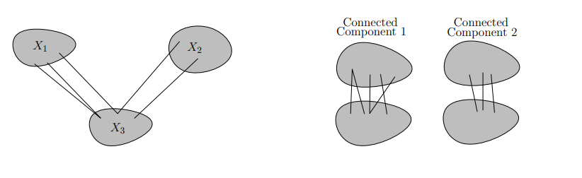
A pair of bonds \(B_1,B_2\) in a graph \(G\) is a modular pair when the number of connected components of \(G\backslash(B_1\cup B_2)\) is exactly two more than the number of connected components of \(G\). Thus \(B_1,B_2\) form a modular pair of bonds when: \(B_1\cup B_2\) forms a tribond, \(B_1\cup B_2\) form the configuration in Figure 1 but with no edges between \(X_1\) and \(X_2\) (see Figure 2, left), or \(B_1\) and \(B_2\) are in two distinct connected components of \(G\) (see Figure 2, right). When \(B_1,B_2\) is a modular pair of bonds but \(B_1\cup B_2\) is not a tribond (i.e., \(B_1\cup B_2\) is one of the structures from Figure 2) we will call \(B_1\cup B_2\) a dibond. Note that a modular pair of bonds is disjoint if and only if their union is a dibond.
The matroid of Theorem 2.3 is \(J_0(G,\mathcal L)\), the complete join matroid of \((G,\mathcal L)\). If \(\mathcal L\) is trivial, then the single-element extension associated with \(\mathcal L\) is just \(M(G)\) along with a new element that is either a loop or coloop.
Theorem 2.3 ([4, Theorem 1]).If \(\mathcal L\) is a non-trivial linear class of bonds of \(G\), then there is a matroid with element set \(E(G)\cup e_0\) in which \(e_0\) is neither a loop nor a coloop and whose cocircuits consist of the following:
(1) bonds in \(\mathcal L\),
(2) sets of the form \(B\cup e_0\) in which \(B\) is a bond not in \(\mathcal L\), and
(3) tribonds and dibonds which do not contain a bond from \(\mathcal L\).
Conversely, if \(N\) is a single-element extension of the graphic matroid \(M(G)\) with new element \(e_0\) which is neither a loop nor a coloop of \(N\), then there is a unique and non-trivial linear class of bonds \(\mathcal L\) of \(G\) such that the cocircuits of \(N\) consist of the sets above.
Consider a partition \(\pi=\{X_1,\ldots,X_k\}\) of \(V(G)\) into nonempty parts such that each induced subgraph \(G[X_i]\) is connected. Such partitions are partially ordered under refinement; specifically, if \(\pi_1\leq\pi_2\) when every block of \(\pi_1\) is a subset of a block of \(\pi_2\). Let \({\rm Lattice}(G)\) denote this partially ordered set of partitions for \(G\).
Given \(\pi=\{X_1,\ldots,X_k\}\in{\rm Lattice}(G)\), denote the set of edges in \(G[X_1]\cup\dots\cup G[X_k]\) by \({\rm Interior}(\pi)\). The set of edges of \(G\) which are not in \({\rm Interior}(\pi)\) is denoted by \({\rm Exterior}(\pi)\). Note that \({\rm Exterior}(\pi)\) is a union of bonds. Given a cobiased graph \((G,\mathcal L)\), we call \(\pi\in{\rm Lattice}(G)\) cobalanced with respect to \(\mathcal L\) when every bond in \({\rm Exterior}(\pi)\) is cobalanced; otherwise the partition is un-cobalanced.
If \(H\) is a subgraph of \(G\), then let \(\pi_H\in{\rm Lattice}(G)\) be the partition of \(V(G)\) given by the connected components of \(H\). If \(J\) is a forest in \((G,\mathcal L)\) for which \(\pi_J\) is cobalanced and \(J\) is minimal with respect to this property, then \(J\) is called an \(\mathcal L\)–join of the cobiased graph \((G,\mathcal L)\). The deletion of any edge of an \(\mathcal L\)-join \(J\) induces a bond that is not in \(\mathcal L\).
Theorem 2.4 ([4, Theorem 9]).If \(\mathcal L\) is a non-trivial linear class of bonds of \(G\), then the circuits of \(J_0(G,\mathcal L)\) consist of the following:
(1) edges sets of the form \(J\cup e_0\) in which \(J\) is an \(\mathcal L\)-join and
(2) edges sets of cycles.
Let \(M\) be a matroid. A pair of circuits \(C_1,C_2\) in \(M\) is a modular pair if and only if \(r(C_1\cup C_2)=|C_1\cup C_2|-2\). A pair of circuits \(C_1,C_2\) are adjacent when the pair is modular and \(M|(C_1\cap C_2)\) is a connected matroid. The reader can verify that if \(C_1,C_2\) is a modular pair of circuits then \(M|(C_1\cap C_2)\) is connected if and only if \(C_1\cap C_2\neq\emptyset\). More generally, if \(C_1,C_2\) is any pair of circuits for which \(C_1\cap C_2\neq\emptyset\), then \(M|(C_1\cap C_2)\) will be connected. The converse, however, need not be true when \(C_1,C_2\) is not modular.
A subset \(\mathcal L\) of the set of circuits of a matroid \(M\) is called a linear class when every modular pair of circuits \(C_1,C_2\) satisfies the property that if \(C_1,C_2\in\mathcal L\) then every circuit of \(M|(C_1\cup C_2)\) is in \(\mathcal L\). Equivalently, either zero, one, or all circuits of \(M|(C_1\cup C_2)\) are in \(\mathcal L\) for every modular pair of circuits \(C_1,C_2\). A simple example of a linear class is the following. Let \(e\in E(M)\) and let \(\mathcal L_e\) denote the set of circuits of \(M\) which do not contain \(e\). Clearly \(\mathcal L_e\) is a linear class.
It is important to note that a modular pair of bonds in a graph \(G\) as we have defined it is exactly a modular pair of circuits in \(M^*(G)\). Now if \(B_1,B_2\) are a modular pair of bonds in \(G\), then \(M^*(G)|(B_1\cup B_2)\) is connected if and only if \(B_1\cap B_2\neq\emptyset\) if and only if \(B_1\cup B_2\) is a tribond as a dibond can only be expressed as a union of disjoint bonds.
A circuit path in a matroid \(M\) is a sequence of circuits \(C_1,\ldots, C_n\) such that \(C_i,C_{i+1}\) are adjacent. If \(\mathcal L\) is a linear class of circuits in \(M\), then a circuit path is off \(\mathcal L\) if each \(C_i\notin\mathcal L\).
Theorem 2.5(Tutte [5, (4.34)]). If \(M\) is a connected matroid and \(\mathcal L\) a linear class of circuits in \(M\), then for each pair of circuits \(C,C'\notin\mathcal L\), there is a circuit path off \(\mathcal L\) from \(C\) to \(C'\).
A pre-orientation of a cobiased graph \((G,\mathcal L)\) is a \(\{-1,0,+1\}\)-valued function \(o\) on the bond boundaries of \(G\) which satisfies the following properties.
(1) If \(B=[X,Y]\) is a cobalanced bond (i.e., \(B\in\mathcal L)\), then \(o(X)=o(Y)=0\).
(2) If \(B=[X,Y]\) is an un-cobalanced bond (i.e., \(B\notin\mathcal L)\), then \(\{o(X),o(Y)\}=\{+1,-1\}\).
(3) If \(T=[X_1,X_2,X_3]\) is a tribond, then either \(o(X_1)=o(X_2)=o(X_3)=0\) or \(\{+1,-1\}\subseteq\{o(X_1),o(X_2),o(X_3)\}\).
Example 3.1. Consider \(K_4\) with vertex labels \(a,b,c,d\). For simplicity of notation we will denote a proper subset of \(\{a,b,c,d\}\) as a string of letters. Since \(K_4\) is complete, every proper subset of \(\{a,b,c,d\}\) is a bond boundary; furthermore, there are six tribonds in \(K_4\) each of which is of the form \([v_1,v_2,v_3v_4]\). Let \(\mathcal L\) be the set containing the following two bonds: \([ab,cd]\) and \([ac,bd]\). Since these two bonds cannot both appear in the same tribond, there is no tribond which contains exactly two bonds from \(\mathcal L\). Thus \((K_4,\mathcal L)\) is a cobiased graph.
Proposition 3.2 and its proof provide an instructive example for pre-orientations. The proposition is, however, implied by the main results of this paper (Theorems 4.2, 4.5, and 4.7) because the single-edge extension of \(M(K_4)\) by linear class \(\mathcal L\) is the non-Fano plane and it is known that the non-Fano plane has only one orientation up to reorientation.
Proposition 3.2. Up to negation \((K_4,\mathcal L)\) has exactly one pre-orientation.
Proof. Let \(o\) be a pre-orientation of \((G,\mathcal L)\). By the definition of pre-orientation, \(-o\) is a pre-orientation as well. Condition (1) implies that \(o(ab)=o(cd)=o(ac)=o(bd)=0\) and Condition (2) implies that these are the only subsets of the vertex set which are zero under \(o\). Also by Condition (2) we may assume up to negation of \(o\) that \(o(ad)=+1\) and \(o(bc)=-1\). Now we need only find the values \(o(a),o(b),o(c),o(d)\) in order to completely determine \(o\).
Using Condition (3) on the tribond \([ad,b,c]\) we must have one of the following three possibilities:
\(\bullet\) \(o(b)=+1\) and \(o(c)=-1\),
\(\bullet\) \(o(b)=-1\) and \(o(c)=+1\), or
\(\bullet\) \(o(b)=o(c)=-1\).
In the first case, we use Condition (3) on tribond \([cd,a,b]\) to obtain \(o(a)=-1\); however, now Condition (3) is contradicted on tribond \([a,c,bd]\). In the second case we also obtain a contradiction in a similar manner. So now assume that \(o(b)=o(c)=-1\). Using Condition (3) on tribond \([a,b,cd]\) yields \(o(a)=+1\) and on tribond \([a,d,bc]\) yields \(o(d)=+1\). The reader can now check that Condition (3) is satisfied on all six tribonds of \((K_4,\mathcal L)\). Thus \(o\) is the only pre-orientation of \((K_4,\mathcal L)\) up to negation. ◻
Example 3.3. Consider again \(K_4\) with vertex labels \(a,b,c,d\). This time let \(\mathcal L\) be the set containing the following three bonds: \([ab,cd]\), \([ac,bd]\), and \([ad,bc]\). As in Example 1, two bonds of \(\mathcal L\) cannot both appear in the same tribond so there is no tribond which contains exactly two bonds from \(\mathcal L\). Thus \((K_4,\mathcal L)\) is a cobiased graph. The single-edge extension of \(M(K_4)\) defined by \(\mathcal L\) is the Fano plane and it is well-known that this matroid is not orientable. Again, the main results of this paper now imply Proposition 3.4 but we provide a direct proof as an illustrative example.
Proposition 3.4. \((K_4,\mathcal L)\) has no pre-orientations.
Proof. Assume by way of contradiction that \(o\) is a pre-orientation of \((G,\mathcal L)\). Thus \(o(v_1v_2)=0\) for all \(\{v_1,v_2\}\subset\{a,b,c,d\}\). Now, by definition of pre-orientations \(-o\) is also a pre-orientation. Thus if we apply Condition (3) to the tribond \([a,b,cd]\), then we may assume without loss of generality that \(o(a)=+1\) and \(o(b)=-1\). Now using the tribond \([a,c,bd]\) we get \(o(c)=-1\). Now on the tribond \([b,c,ad]\) we have \(o(b)=o(c)=-1\) and \(o(ad)=0\) which contradicts Condition (3). ◻
Example 3.5. [Pre-orientations from real quotient labelings] Let \(\pi\colon V(G)\to\mathbb R\) be a quotient labeling of \(G\). Then for each bond \(B=[X,Y]\) define \(o_\pi(X)\) to be \(+1\), \(-1\), or \(0\) according to whether \(\pi(X)>0\), \(\pi(X)<0\), or \(\pi(X)=0\) respectively.
Proposition 3.6. If \(\pi\colon V(G)\to\mathbb R\) is a quotient labeling of \(G\), then \(o_\pi\) is a pre-orientation.
Proof. Consider a bond \([X,Y]\). Conditions (1) and (2) for \(o_\pi\) are satisfied because \(\pi(X)+\pi(Y)=0\). For a tribond \([X_1,X_2,X_3]\) Condition (3) for \(o_\pi\) is satisfied because \(\pi(X_1)+\pi(X_2)+\pi(X_3)=0\). ◻
An orientation of a cobiased graph \((G,\mathcal L)\) is a pair \((o,\tau)\) in which \(o\) is a pre-orientation of \((G,\mathcal L)\) and \(\tau\) is an orientation of \(G\).
For each cocircuit \(C\) of \(J_0(G,\mathcal L)\), an orientation \((o,\tau)\) will produce two signed cocircuits \([o,\tau,C]\) and \(-[o,\tau,C]\) which are defined as follows.
(1) If \(C\) is a balanced bond, then arbitrarily choose one direction across the bond. Now \(e\in[o,\tau,C]_+\) when \(e\) under \(\tau\) is in the chosen direction across \(B\); otherwise, \(e\in[o,\tau,C]_-\).
(2) If \(C=B\cup e_0\) in which \(B=[X,Y]\) is an un-cobalanced bond with \(o(X)=+1\), then \(e\in[o,\tau,C]_+\) when \(e=e_0\) or the head of \(e\) under \(\tau\) is in \(X\); otherwise, \(e\in[o,\tau,C]_-\).
(3) Let \(C\) be a dibond \([X_1,Y_1]\cup[X_2,Y_2]\) with \(X_1\cap X_2=\emptyset\).
\(\bullet\) If \(o(X_1)=o(X_2)\), then \(e\in[o,\tau,C]_+\) when the head of \(e\) is in \(X_1\) or the tail of \(e\) is in \(X_2\); otherwise, \(e\in[o,\tau,C]_-\).
\(\bullet\) If \(o(X_1)\neq o(X_2)\), then \(e\in[o,\tau,C]_+\) when the head of \(e\) is in \(X_1\) or the head of \(e\) is in \(X_2\); otherwise, \(e\in[o,\tau,C]_-\).
(4) If \(C\) is a tribond \([X_1,X_2,X_3]\) with \(o(X_1)=o(X_2)\), then \(e\in[o,\tau,C]_+\) when the head of \(e\) is in \(X_1\) or the tail of \(e\) is in \(X_2\); otherwise, \(e\in[o,\tau,C]_-\).
For each circuit \(C\) of \(J_0(G,\mathcal L)\), an orientation \((o,\tau)\) will produce two signed cocircuits \([o,\tau,C]\) and \(-[o,\tau,C]\); however, before we can define \([o,\tau,C]\), we need to establish a property of \(\mathcal L\)-joins.
Let \(o\) be a pre-orientation of \((G,\mathcal L)\), \(J\) an \(\mathcal L\)-join of \((G,\mathcal L)\), and \(e\in J\). Because \(\pi_J\) is cobalanced and \(\pi_{J\backslash e}\) is un-cobalanced, a bond in \({\rm Exterior}(\pi_{J\backslash e})\) is un-cobalanced if and only if it contains \(e\). Let \(B=[X,Y]\) be such a bond and say without loss of generality that \(o(X)=-1\). Define \((B,o,J,e)\) to be the orientation of \(e\) whose head is in \(X\). In Proposition 4.1 we show that \((B,o,J,e)\) is independent of \(B\) and so we denote this orientation of \(e\) with respect to \(J\) and \(o\) by \((o,J,e)\).
Proposition 4.1. For any two bonds \(B_1\) and \(B_2\) in \({\rm Exterior}(\pi_{J\backslash e})\) both containing \(e\), \((B_1,o,J,e)=(B_2,o,J,e)\).
Proof. First, assume that \(B_1,B_2\) is a modular pair of bonds in \(G\). Since \(e\in B_1\cap B_2\) it must be that \(B_1\cup B_2\) is a tribond because \(B_1\cap B_2=\emptyset\) when \(B_1\cup B_2\) is a dibond. Let \([X_1,X_2,X_3]\) denote this tribond. Say without loss of generality that \(B_1=[X_1,X_2\cup X_3]\) and \(B_2=[X_2,X_1\cup X_3]\). Bonds \(B_1\) and \(B_2\) are both un-cobalanced, but bond \([X_3,X_1\cup X_2]\) does not contain \(e\) and so is cobalanced. Thus \(o(X_1)=+1\), \(o(X_2)=-1\), and \(o(X_3)=0\) which makes \((B_1,o,J,e)=(B_2,o,J,e)\), as required.
Now suppose that \(B_1,B_2\) is not a modular pair of bonds. Since \(e\in B_1\cap B_2\), \(M^*(G)|(B_1\cup B_2)\) is a connected matroid. Let \(\mathcal L_e\) be the linear class of bonds in \(M^*(G)|(B_1\cup B_2)\) that do not contain \(e\). By Theorem 2.5 there is a path of adjacent bonds \(A_1,\ldots,A_t\) with \(A_1=B_1\), \(A_t=B_2\), and \(A_i\notin\mathcal L_e\) for each \(i\). Now \((A_i,o,J,e)=(A_{i+1},o,J,e)\) by the argument in the previous paragraph and our result follows. ◻
Now for a circuit \(C\) of \(J_0(G,\mathcal L)\) we define the signed circuit \([o,\tau,C]\) as follows.
(1) If \(C\) is a cycle in \(G\), then arbitrarily choose one direction along \(C\). Now \(e\in [o,\tau,C]_+\) when \(e\) under \(\tau\) is in the chosen direction around \(C\); otherwise, \(e\in[o,\tau,C]_-\).
(2) If \(C=J\cup e_0\) in which \(J\) is an \(\mathcal L\)-join, then \(e\in[o,\tau,C]_+\) when \(e=e_0\) or when \(e\) under \(\tau\) is in the direction of \((o,J,e)\); otherwise, \(e\in[o,\tau,C]_-\).
Theorem 4.2(Main Result 1).If \((o,\tau)\) is an orientation of cobiased graph \((G,\mathcal L)\), then the circuit signature given by \((o,\tau)\) is an orientation of \(J_0(G,\mathcal L)\) and the cocircuit signature given by \((o,\tau)\) is the dual orientation of \(J_0^*(G,\mathcal L)\).
Proof. Let \(C\) be a circuit and \(D\) a cocircuit of \(J_0(G,\mathcal L)\). The signed circuit \([o,\tau,C]\) and signed cocircuit \([o,\tau,D]\) are orthogonal when \[\big([o,\tau,C]_+\cap [o,\tau,D]_-\big)\cup\big([o,\tau,C]_-\cap [o,\tau,D]_+\big)\neq\emptyset,\]and\[\big([o,\tau,C]_+\cap [o,\tau,D]_+\big)\cup\big([o,\tau,C]_-\cap [o,\tau,D]_-\big)\neq\emptyset.\]
In order to prove our theorem, we need to show that for each circuit \(C\) and cocircuit \(D\) with \(2\leq|C\cap D|\leq3\) that \([o,\tau,C]\) and \([o,\tau,D]\) are orthogonal. (See, for example, [1, Theorem 3.4.3].)
In Case 1 say that \(D\backslash e_0\) is a bond and in Case 2 that \(D\) is a dibond or tribond.
Case 1. If \(C\) is a cycle, then we may write \(C\cap D=\{e_1,e_2\}\); furthermore, \(e_1,e_2\) have the same sign in \([o,\tau,D]\) if and only if \(e_1\) and \(e_2\) point in the same direction across the bond while \(e_1,e_2\) have the same sign in \([o,\tau,C]\) if and only if \(e_1\) and \(e_2\) point in different directions across the bond. Thus \([o,\tau,C]\) and \([o,\tau,D]\) are orthogonal.
For the rest of Case 1 we may now assume that \(C=J\cup e_0\) in which \(J\) is an \(\mathcal L\)-join. Let \(B\) denote the bond \(D\backslash e_0\) and write \(B=[X,Y]\). Note that if \(T\) is a connected component of \(J\) which is contained in \(G[X\cup Y]\), then either \(E(T)\cap B\neq\emptyset\) or \(V(T)\subseteq X\) or \(V(T)\subseteq Y\). Now because \(G[X]\cup G[Y]\cup(B\cap J)\) is connected, \(J\) can be extended to a maximal forest \(F\) of \(G\) without using edges of \(B\backslash J\). Let \(T_0\) be the tree in \(F\) which spans \(G[X\cup Y]\). Now split this case into three subcases according to the value \(|B\cap J|\in\{1,2,3\}\).
Case 1.1. Since \(|B\cap J|=1\) and \(2\leq|C\cap D|\leq3\), it must be that \(D=B\cup e_0\). Let \(e\) denote the element of \(B\cap J\). Thus \(e_0\in[o,\tau,C]_+\cap [o,\tau,D]_+\) and \(e\in[o,\tau,C]_\sigma\cap [o,\tau,D]_{-\sigma}\). Thus \([o,\tau,C]\) and \([o,\tau,D]\) are orthogonal.
Case 1.2. Suppose that \(|B\cap J|=2\). Say \(B\cap J=\{e_1,e_2\}\). Without loss of generality \(T_0\backslash\{e_1,e_2\}\) has three connected components with vertex sets \(X,Y_1,Y_2\) as shown in Figure 5 where \(Y_1\cup Y_2=Y\).
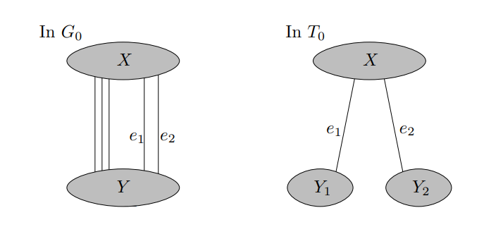
Thus \([X,Y_1,Y_2]\) is a tribond and bonds \([X\cup Y_1,Y_2]\) and \([X\cup Y_2,Y_1]\) are both un-cobalanced because \(e_i\in J\).
If \(B\) is cobalanced, then \(o(Y_1)=-o(Y_2)\). Thus \(e_1,e_2\) have the same sign in \([o,\tau,C]\) if and only if they point in different directions across \(B\) and \(e_1,e_2\) have the same sign in \([o,\tau,D]\) if and only if they point in the same direction across \(B\). Thus \([o,\tau,C]\) and \([o,\tau,D]\) are orthogonal.
If \(B\) is un-cobalanced, then either \(o(Y_1)=-o(Y_2)\) or \(o(Y_1)=o(Y_2)\). In the former case, \([o,\tau,C]\) and \([o,\tau,D]\) are orthogonal as in the previous paragraph. In the latter case \(e_0\) and \(e_1\) have the same sign in \([o,\tau,D]\) if and only if \(e_1\) has its head in the positive bond boundary of \(B=[X,Y]\) while \(e_0\) and \(e_1\) have the same sign in \([o,\tau,C]\) if and only if \(e_1\) has its head in the negative bond boundary of \(B=[X,Y]\). Thus \([o,\tau,C]\) and \([o,\tau,D]\) are orthogonal.
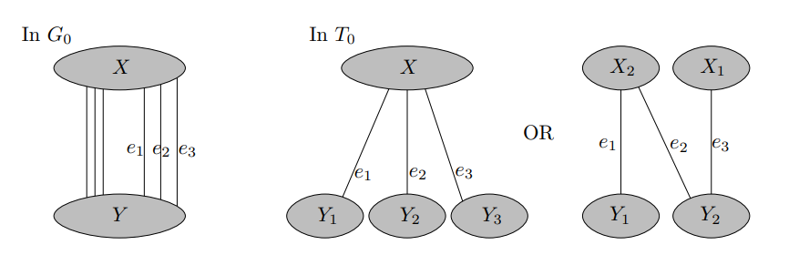
Case 1.3. Suppose that \(|B\cap J|=3\). Since \(|C\cap D|\leq3\) we must have that \(B\) is cobalanced. Let \(e_1,e_2,e_3\) denote the edges of \(B\cap J\). Now the four vertex sets of the connected components of \(T_0\backslash\{e_1,e_2,e_3\}\) have two possible structures as shown in Figure 6 where \(Y=Y_1\cup Y_2\cup Y_3\) in the first case and \(Y=Y_1\cup Y_2\) and \(X=X_1\cup X_2\) in the second case. Let these be Cases 1.3.1 and 1.3.2.
Case 1.3.1. Here \(B=[X,Y_1\cup Y_2\cup Y_3]\). Now \(e_i\) and \(e_j\) have the same sign in \([o,\tau,D]\) if and only if they point in the same direction across \(B\). The values of \(o(Y_1),o(Y_2),o(Y_3)\) are all non-zero because \(e_1,e_2,e_3\in J\). If two are different (say \(o(Y_1)=-o(Y_2)\)), then \(e_1\) and \(e_2\) have the same sign in \([o,\tau,C]\) if and only if they point in opposite directions across \(B\). Thus \([o,\tau,C]\) and \([o,\tau,D]\) would be orthogonal.
So now suppose by way of contradiction that \(o(Y_1)=o(Y_2)=o(Y_3)=+1\) without loss of generality. Because \(Y=Y_1\cup Y_2\cup Y_3\) and \(G[Y]\) is connected, there is without loss of generality an edge from \(Y_2\) to \(Y_1\) and an edge from \(Y_2\) to \(Y_3\). Consider the tribond \([X,Y_1,Y_2\cup Y_3]\). Because \(o(X)=0\) and \(o(Y_1)=+1\), we get that \(o(Y_2\cup Y_3)=-1\). This now implies that \(o(X\cup Y_1)=+1\). Now \([X\cup Y_1,Y_2,Y_3]\) is a tribond; however, \(o(X\cup Y_1)=o(Y_2)=o(Y_3)=+1\), a contradiction.
Case 1.3.2. In this case \(B=[X_1\cup X_2,Y_1\cup Y_2]\). Edges \(e_i\) and \(e_j\) have the same sign in \([o,\tau,D]\) if and only if they point in the same direction across \(B\). Now \(o(X_1),o(Y_1)\neq0\). If \(o(X_1)=o(Y_1)\), then \(e_1\) and \(e_3\) have the same sign in \([o,\tau,C]\) if and only if they point in opposite directions across \(B\). In this case \([o,\tau,C]\) and \([o,\tau,D]\) would be orthogonal. So assume without loss of generality that \(o(X_1)=-o(Y_1)=+1\). Consider the tribond \([X_1,X_2,Y_1\cup Y_2]\). Because \(Y=Y_1\cup Y_2\) and \(o(Y)=0\) we get that \(o(X_2)=-1\). We can similarly use the tribond \([X_1\cup X_2,Y_1,Y_2]\) to obtain \(o(Y_2)=+1\). Now use the tribond \([X_1\cup Y_2,X_2,Y_1]\) to obtain \(o(X_1\cup Y_2)=+1\). Now \(e_2\) and \(e_3\) have the same sign in \([o,\tau,C]\) if and only if they point opposite directions across \(B\). Thus \([o,\tau,C]\) and \([o,\tau,D]\) are orthogonal.
Case 2. Clearly orthogonality is invariant under reorientation of \(\tau\). Thus we may assume that \([o,\tau,D]\) is all positive. By our definition of cocircuit signatures (and without loss of generality) \(D=B_1\cup B_2\) in which \(B_1,B_2\) is a modular pair of bonds for which \([o,\tau,B_1\cup e_0]\) is all positive and \(-[o,\tau,B_2\cup e_0]\) is all positive except for \(e_0\). By Case 1, \([o,\tau,C]\) is orthogonal to both \([o,\tau,B_1\cup e_0]\) and \(-[o,\tau,B_2\cup e_0]\). If \(C\) is a cycle, then \([o,\tau,C]\) must be orthogonal to at least one of the signed bonds \([o,\tau,B_i\cup e_0]\backslash e_0\) and hence \([o,\tau,C]\) and \([o,\tau,D]\) are orthogonal. If \(C=J\cup e_0\), then orthogonality with each \([o,\tau,B_i\cup e_0]\) implies that there is \(e_1\in B_1\) for which \(e_1\in[o,\tau,C]_-\) and \(e_2\in B_2\) for which \(e_2\in[o,\tau,C]_+\). Thus \([o,\tau,C]\) and \([o,\tau,D]\) are orthogonal. ◻
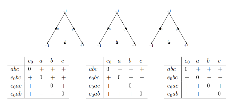
Example 4.3. The matroid \(J_0(K_3,\emptyset)\) is the uniform matroid \(U_{2,4}\). Up to reorientation, there are three orientations of a labeled copy of \(U_{2,4}\). The three orientations of \((K_3,\emptyset)\) shown in Figure 7 produce the cocircuit signatures given below which are pairwise unequal up to reorientation.
| \(e_0\) | \(a\) | \(b\) | \(c\) | |
|---|---|---|---|---|
| \(abc\) | 0 | \(+\) | \(+\) | \(+\) |
| \(e_0bc\) | \(+\) | 0 | \(+\) | \(+\) |
| \(e_0ac\) | \(+\) | \(-\) | 0 | \(+\) |
| \(e_0ab\) | \(+\) | \(-\) | \(-\) | 0 |
| \(e_0\) | \(a\) | \(b\) | \(c\) | |
|---|---|---|---|---|
| \(abc\) | 0 | \(+\) | \(+\) | \(+\) |
| \(e_0bc\) | \(+\) | 0 | \(+\) | \(-\) |
| \(e_0ac\) | \(+\) | \(-\) | 0 | \(-\) |
| \(e_0ab\) | \(+\) | \(+\) | \(+\) | 0 |
| \(e_0\) | \(a\) | \(b\) | \(c\) | |
|---|---|---|---|---|
| \(abc\) | 0 | \(+\) | \(+\) | \(+\) |
| \(e_0bc\) | \(+\) | 0 | \(-\) | \(-\) |
| \(e_0ac\) | \(+\) | \(+\) | 0 | \(+\) |
| \(e_0ab\) | \(+\) | \(+\) | \(-\) | 0 |
If \(\tau\) is an orientation of a graph \(G\), then denote the reorientation of \(\tau\) on \(X\subseteq E(G)\) by \(\tau_X\). Now let \((o,\tau)\) be an orientation \((G,\mathcal L)\) and \(\mathfrak O(o,\tau)\) denote the orientation of \(J_0(G,\mathcal L)\) given by \((o,\tau)\). The reorientation of \(\mathfrak O(o,\tau)\) on \(X\subseteq E(G)\) is clearly given by \(\mathfrak O(o,\tau_X)\) according to our definition of cocircuit signatures. Furthermore, as with any general oriented matroid, the reorientation of \(\mathfrak O(o,\tau)\) on \(X\cup e_0\) is the same as the reorientation of \(\mathfrak O(o,\tau)\) on \(E(G)\backslash X\). Thus reorientations of \(\tau\) on subsets of \(E(G)\) are enough to describe all reorientations \(\mathfrak O(o,\tau)\).
Proposition 4.4. If \(o\) is a pre-orientation of \((G,\mathcal L)\), then any two orientations of \(J_0(G,\mathcal L)\) given by \(o\) and \(-o\) are equal up to reorientation.
Proof. The reorientation of \(\mathfrak O(o,\tau)\) on \(e_0\) is \(\mathfrak O(o,\tau_{E(G)})\) which according to our definition of cocircuit signatures is \(\mathfrak O(-o,\tau)\). This implies our result. ◻
Theorem 4.5(Main Result 2). Let \(G\) be a 2-connected simple graph. If \(o_1\) and \(o_2\) are pre-orientations of \((G,\mathcal L)\), then any two orientations of \(J_0(G,\mathcal L)\) given by \(o_1\) and \(o_2\) are equal up to reorientation if and only if \(o_1=\pm o_2\).
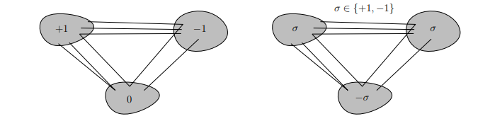
Proof. The easier direction is given by Proposition 4.4. So now assume that \(o_1\neq\pm o_2\). This means that there are un-cobalanced bonds \(B=[X,Y]\) and \(B'=[X',Y']\) for which \(o_1(X)=o_2(X)\) and \(o_1(X')\neq o_2(X')\). Since \(G\) is 2-connected and simple \(M^*(G)\) is connected. Theorem 2.5 implies that there is a path of un-cobalanced bonds \(A_1,\ldots,A_t\) for which \(B=A_1\), \(B'=A_t\), and \(A_i\cup A_{i+1}\) is a tribond. Thus there is \(i\) for which \(o_1\) and \(o_2\) agree on \(A_i\) and disagree on \(A_{i+1}\). Note that this requires that the tribond \(A_i\cup A_{i+1}\) does not contain any balanced bonds. So without loss of generality, \(o_1\) and \(o_2\) on the tribond \(A_{i}\cup A_{i+1}\) are as shown in Figure 8.
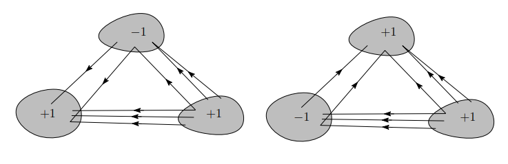
The simplification of \(J_0^*(G,\mathcal L)|(A_i\cup A_{i+1})\) is \(U_{2,4}\) and so the cocircuit signatures given by the orientations in Figure 8 on the parallel classes of elements of \(J_0^*(G,\mathcal L)|(A_i\cup A_{i+1})\) are as shown in Figure 7. Thus any two orientations given by \(o_1\) and \(o_2\) are unequal up to reorientation on \(J_0^*(G,\mathcal L)|(A_i\cup A_{i+1})\) and hence on the whole of \(J_0^*(G,\mathcal L)\) and \(J_0(G,\mathcal L)\). ◻
There are examples of cobiased graphs for which there are only two pre-orientations \(o\) and \(-o\). Example 3.1 of Section 3 is one such cobiased graph. The canonical example, however, is an additively cobiased graph. A cobiased graph \((G,\mathcal L)\) additively cobiased when every tribond contains either one or three cobalanced bonds (i.e., never contains zero cobalanced bonds).
Theorem 4.6. If \(G\) is a 2-connected graph and \((G,\mathcal L)\) is additively cobiased and has a pre-orientation \(o\), then \(o\) and \(-o\) are the only pre-orientations of \((G,\mathcal L)\).
Proof. Let \(o_1\) and \(o_2\) be pre-orientations on \((G,\mathcal L)\) and \(B=[X,Y]\) be an un-cobalanced bond. Using negation, assume that \(o_1(X)=o_2(X)\). Now for any other un-cobalanced bond \(B'\) in \((G,\mathcal L)\) we may use Theorem 2.5 as in the proof of Theorem 4.5 to show that \(o_1\) and \(o_2\) are equal on the bond boundaries of \(B'\). ◻
Our final result it Theorem 4.7. This result combined with Theorems 4.2 and 4.5 tell us that every orientation of any single-element extension of a graphic matroid is uniquely uniquely represented by an orientation \((o,\tau)\) of the associated cobiased graph \((G,\mathcal L)\) up to negation of \(o\).
Theorem 4.7(Main Result 3). Every orientation of \(J_0(G,\mathcal L)\) is given by an orientation \((o,\tau)\) of \((G,\mathcal L)\).
Proof. Let \(\mathfrak O\) be an oriented matroid whose underlying matroid is \(J_0(G,\mathcal L)\). Thus \(\mathfrak O\backslash e_0\) is an orientation of \(M(G)\) and there are exactly two orientations of \(G\), say \(\tau\) along with its reversal \(\tau_{E(G)}\), which represent \(\mathfrak O\backslash e_0\). Now let \(B=[X,Y]\) be an un-cobalanced bond of \((G,\mathcal L)\) and let \(\hat B\) be the signing of cocircuit \(B\cup e_0\) in \(\mathfrak O\) in which \(e_0\) is positive. Without loss of generality the edges of \(B\) which are positive in \(\hat B\) have their heads in \(X\) and the edges of \(B\) which are negative have their heads in \(Y\). Define \(o(X)=+1\) and \(o(Y)=-1\). For any cobalanced bond, define \(o\) to be zero on both bond boundaries. We have now defined \(o\) on all bond boundaries. We claim that \(o\) is a pre-orientation and that \((o,\tau)\) determines \(\mathfrak O\). The latter will be done by checking that the cocircuit signatures of \(\mathfrak O\) are given by \((o,\tau)\) which we have just established for both the cobalanced and un-cobalanced bonds.
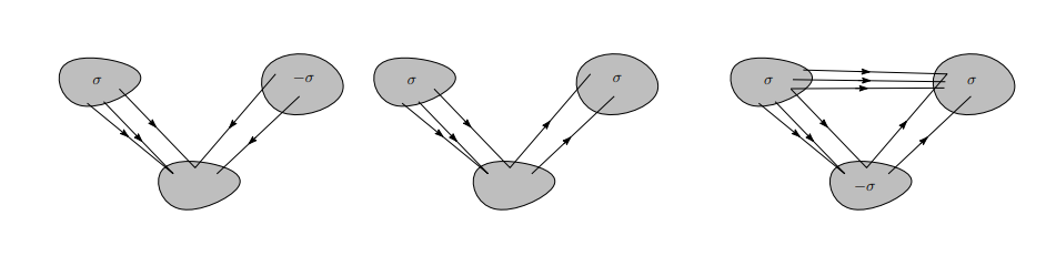
Consider a dibond \(D=B_1\cup B_2\) where \(B_i=[X_i,Y_i]\) and \(X_1\cap X_2=\emptyset\). Reorient \(\mathfrak O\) on the edges of \(B_1\) so that one of the signings on \(B_1\cup e_0\) is all positive, call it \(\hat B_1\). Reorient the edges of \(B_2\) (which are disjoint from \(B_1\)) so that one of the signings on \(B_2\cup e_0\) is all positive except for \(e_0\), call it \(\hat B_2\). We have already established that the signatures on \(\hat B_1\) and \(\hat B_2\) are given by \((o,\tau)\). Thus the edges of \(B_i\) are all in the same direction across the bond. Now by signed circuit exchange using \(\hat B_1\), \(\hat B_2\), and \(e_0\), we get an all-positive signing of \(D\) in \(\mathfrak O\). Thus according to our definition of cocircuit signatures on dibonds, this signature on \(D\) is given by \((o,\tau)\) (see Figure 4).
Finally, consider a tribond \([X_1,X_2,X_3]\). Without loss of generality, we need only consider the case in which \(o(X_1)=o(X_2)=+1\). Reorient \(\mathfrak O\) on the edges in \([X_1,X_2,X_3]\) so that the corresponding reorientation of \(\tau\) has every edge with either its head in \(X_1\) or its tail in \(X_2\). Since the cocircuit signatures of \([X_1,X_2\cup X_3]\cup e_0\) and \([X_2,X_1\cup X_3]\cup e_0\) in \(\mathfrak O\) are given by \((o,\tau)\), there are signed cocircuits \(\hat B_1\) and \(\hat B_2\) on \(B_1\cup e_0\) and \(B_2\cup e_0\) for which \(\hat B_1\) is all positive and \(\hat B_2\) is all positive save for \(e_0\). Using signed circuit exchange on \(e_0\), \(\mathfrak O\) contains an all-positive signed cocircuit on a subset of \([X_1,X_2,X_3]\). The only possible cocircuits in the tribond \([X_1,X_2,X_3]\) are the tribond itself when \([X_3,X_1\cup X_2]\) is un-cobalanced and the bond \([X_3,X_1\cup X_2]\) when it is cobalanced. The latter case, however, is not possible because the edges of \([X_3,X_1\cup X_2]\) are not all in the same direction under \(\tau\). Thus the tribond \([X_1,X_2,X_3]\) is a cocircuit whose signing is all positive. It remains only to show that \(o(X_3)=-1\). Consider the signed cocircuits \(\hat B_1\) and \(-\hat B_2\). Using signed circuit exchange on any edge \(e\) between \(X_1\) and \(X_2\), the signing on cocircuit \([X_3,X_1\cup X_2]\cup e_0\) has \(e_0\) positive, the edges between \(X_1\) and \(X_3\) positive and the edges between \(X_2\) and \(X_3\) negative. Since we have established that this signing is given by \((o,\tau)\), it must be that \(o(X_3)=-1\), as required. ◻
A theta graph consists of two vertices \(u\) and \(v\) along with three internally disjoint \(uv\)-paths. A theta graph has exactly three cycles in it. A linear class of cycles in a graph \(G\) is a subset \(\mathcal L\) of the cycles of \(G\) in which each theta subgraph contains either zero, one, or three cycles from \(\mathcal L\); that is, no theta subgraph contains exactly two cycles from \(\mathcal L\). A biased graph is a pair \((G,\mathcal L)\) in which \(G\) is a graph and \(\mathcal L\) is a linear class of cycles of \(G\).
Given a connected graph \(G\) embedded in the plane, let \(G^*\) denote its topological dual graph. The edges of \(G\) and \(G^*\) are in bijective correspondence; however, for simplicity we will denote them using the same edge set. The correspondence between edges extends to a bijection between the set of bonds of \(G\) and the set of cycles of \(G^*\). Thus \(M^*(G)=M(G^*)\). This is the easy direction of Whitney’s Theorem (Theorem 1.1). In addition to this correspondence between bonds in \(G\) and cycles in \(G^*\), the topology of the plane also implies that there is a correspondence between tribonds in \(G\) and theta graphs in \(G^*\). This correspondence yields Proposition 5.1.
Proposition 5.1. Let \(G\) be a connected graph embedded in the plane. A collection of bonds \(\mathcal L\) in \(G\) is a linear class if and only if \(\mathcal L\) is a linear class of cycles of \(G^*\).
Given a biased graph \((G,\mathcal L)\), the coextension of \(M(G)\) by a single element \(e_0\) is the matroid \(L_0(G,\mathcal L)\) whose circuits are the edge sets of the following:
(1) cycles in \(\mathcal L\),
(2) sets of the form \(C\cup e_0\) where \(C\) is a cycle not in \(\mathcal L\),
(3) the union of two cycles \(C_1,C_2\) which are not in \(\mathcal L\) and which intersect in at most a single vertex, and
(4) theta graphs which contain no cycles in \(\mathcal L\).
Proposition 5.2. If \((G,\mathcal L)\) is a cobiased graph in which \(G\) is connected and embedded in the plane, then \(J_0^*(G,\mathcal L)=L_0(G^*,\mathcal L)\).
Proof. By Proposition 5.1, \((G^*,\mathcal L)\) is a biased graph. The topology of the plane now implies the following correspondence between the following edge sets in \((G,\mathcal L)\) with those in \((G^*,\mathcal L)\): balanced bonds to balanced cycles, unbalanced bonds to unbalanced cycles, dibonds without balanced bonds to sets of type (3) above, and tribonds without balanced bonds to theta graphs without balanced cycles. The result follows. ◻
At this point we will assume at this point that the reader has access to [3] and has become familiar with orientations of biased graphs and their associated complete lift matroids. Again, let \((G,\mathcal L)\) be a cobiased graph in which \(G\) is connected and embedded in the plane and let \(o\) be a pre-orientation of \((G,\mathcal L)\). Given an unbalanced cycle \(C\) of \(G^*\), let \(X,Y\) be the bipartition of \(V(G)\) into non-empty subsets given by \(C\). Since \(C\) is the set of edges of an unbalanced bond with \(X\) and \(Y\) as its boundary sets, we may assume without loss of generality that \(o(X)=+1\) and \(o(Y)=-1\). Since \(G\) is embedded in the plane, so is \(C\). If \(X\) corresponds to the inner region of \(C\), then define \(o^*(C)\) as the clockwise orientation of \(C\); otherwise, define \(o^*(C)\) as the counter-clockwise orientation of \(C\). Now if \(\tau\) is an orientation of \(G\), then define \(\tau^*\) to be the orientation of \(G^*\) obtained by choosing for each \(e\) the orientation of \(e\) in \(G^*\) obtained via a counter-clockwise rotation of the corresponding oriented edge given by \(\tau\) in \(G\). Theorem 5.3 now follows by checking that the signings on the cocircuits of \(J_0(G,\mathcal L)\) given by \((o,\tau)\) are the same as the signings of the corresponding circuits of \(L_0(G,\mathcal L)\) given by \((o^*,\tau^*)\). In fact, one need only check an arbitrary cocircuit’s signing under \((o,\tau)\) is all-positive if and only if its corresponding circuit has an all-positive signing under \((o^*,\tau^*)\).
Theorem 5.3. Let \((G,\mathcal L)\) be a cobiased graph in which \(G\) is connected and planar. If \((o,\tau)\) is an orientation of \((G,\mathcal L)\), then \((o^*,\tau^*)\) is an orientation of \((G^*,\mathcal L)\) and the oriented matroids obtained from \((o,\tau)\) and \((o^*,\tau^*)\) are dual oriented matroids.