
As outlined in [9], graph labeling was introduced in the 1960s and has since had over 2000 papers published on over 200 different types of labelings. Probably the most popular and well-known vertex labeling of graphs would be graph coloring as in the four color theorem. When zero-divisor graphs were first defined by I. Beck in 1988 in [6], the coloring number was the focus. The initial definition of zero-divisor graph has been refined slightly since then by D.F. Anderson and P.D. Livingston in [3] so that for any commutative ring \(R\) with non-trivial zero-divisors, the zero-divisor graph is denoted \(\Gamma(R)\). It has a vertex set \(V(\Gamma(R))=Z(R)^*\), the nonzero zero-divisors (Beck included \(0\) as well as every element of \(R\) as a vertex), and distinct vertices \(x\) and \(y\) are adjacent if and only if \(xy=0\). We will generally also suppose these rings are not integral domains so that there are nonzero zero-divisors to make the zero-divisor graph non-empty. Zero-divisor graphs have been studied by many authors including, but not limited to D.D. Anderson, D.F. Anderson, M. Axtell, A. Badawi, A. Frazier, J. Stickles, A. Lauve, P.S. Livingston, M. Naseer and the second author in [1, 2, 3, 4, 7, 5, 13, 12].
Zero-divisor graphs have been investigated for the existence of various graph labelings. In particular, the second author has explored graceful and harmonious labelings of zero-divisor graphs in [14], magic type labelings in [18], and cordial labelings in [9]. Thus, in this article, we continue this program of examining important vertex and edge labelings of zero-divisor graphs. There are many known properties of zero-divisor graphs which make them excellent candidates for studying their labelings and will be useful later in this article. These include statements on whether \(\Gamma(R)\) is finite, connected, and bounds for the diameter and girth of the graph. Recall that the diameter, denoted \(Diam(G)\), is the largest distance between any two vertices of a graph, and the girth \(gr(G)\) is the length of the shortest cycle.
Theorem 1.1. Let \(R\) be a commutative ring with unity, \(1\neq0\). Then we have the following
(1) ([3, Theorem 2.2]) \(V(\Gamma(R))\) is finite if and only if \(R\) is finite or \(R\) is an integral domain.
(2) ([3, Theorem 2.3]) \(\Gamma(R)\) is connected and Diam\((\Gamma(R)) \leq 3\).
(3) ([3, Theorem 2.4]) Let \(R\) be a commutative Artinian ring. Then if \(\Gamma(R)\) contains a cycle, then gr\((\Gamma(R)) \leq 4\).
The particular graph labeling we investigate is called a prime labeling. It was first introduced by Tout, Dabboucy, and Howalla in 1982 in [1] and has been examined for numerous classes of graphs within dozens of papers, as seen in Gallian’s survey on graph labeling [9]. Let \(G\) be a simple undirected graph with vertex set \(V\) such that \(|V|=n\). Then a prime labeling is a vertex labeling using all of the integers from \(1\) to \(n\) such that the labels of any two adjacent vertices are relatively prime. More formally, a prime labeling is a bijection \(\ell:V \to \{1, 2, \ldots, n\}\) such that any adjacent \(x,y \in V\) satisfy \(\gcd(\ell(x),\ell(y))=1\). A graph \(G\) that admits such a labeling is called prime. This is a natural direction of study for zero-divisor graphs since graph coloring, a focus of the initial work on these graphs, can be viewed as labeling vertices with integers representing the colors such that adjacent vertices have nonequal labels. Prime labelings can be considered an extension of graph coloring by strengthening the nonequal condition to now require adjacent vertices to not share any common factors while relaxing the available labeling set to include integers up to \(|V|\).
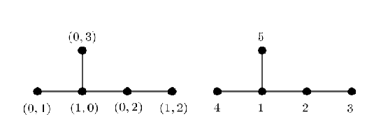
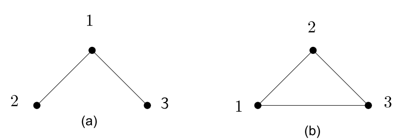
An example of a zero-divisor graph for the ring \(\mathbb{Z}_2\times \mathbb{Z}_4\), along with a prime labeling assigned to its vertices, see Figure 1.
The dual notion to prime labeling is called vertex prime labeling and was developed by Deretsky, Lee, and Mitchem in 1991 in [21]. A graph \(G\) with edge set \(E\) where \(|E| =q\) is said to be vertex prime if there is an edge labeling using all of the integers from \(1\) to \(q\) such that for every vertex of degree at least \(2\), the greatest common divisor of the labels of all incident edges is \(1\). Note, this is not to say they are all pairwise coprime, but rather the largest integer which divides every incident edge’s label is \(1\).
The paper is organized as follows. In Section 2, we briefly address the question of whether zero-divisor graphs are vertex prime, and then present several theorems which will yield infinite classes of commutative rings which have prime zero-divisor graphs. We also show that we can find infinitely many rings with finite zero-divisor graphs, yet do not admit a prime labeling. Finally, in Section 3 we go through Redmond’s work in [16, 17] where he has found every zero-divisor graph with up to 14 vertices and determine which graphs are prime. We conclude the article with multiple conjectures and open questions about zero-divisor graphs and prime labelings.
In our first result, we quickly resolve the question about which commutative rings have zero-divisor graphs which are vertex prime. We have the following from [21], which directly proves the resulting corollary by Theorem 1.1(2).
Theorem 2.1. ([21, Corollary 4]) All finite, connected graphs are vertex prime.
Corollary 2.2. Let \(R\) be a finite commutative ring with unity which is not an integral domain. Then \(\Gamma(R)\) is vertex prime.
Again, since every finite zero-divisor graph is always connected, this resolves the question about whether any zero-divisor graph is vertex prime in the affirmative, and we only include this type of labeling for the sake of completeness.
We now turn our attention to trying to answer the question for prime labelings. With this in mind, we summarize known results about this more interesting labeling condition for zero-divisor graphs in the following theorem. Proofs can be found in [1] for (1), in [8] for (2), and in [11] for (3) and (4).
Theorem 2.3. We have the following classification results for various types of graphs
(1) The complete graph \(K_n\) is prime if and only if \(n \leq 3\).
(2) The star graph \(K_{1,n}\) is prime for all \(n\).
(3) The complete bipartite graph \(K_{2,n}\) is prime for all \(n\).
(4) The complete bipartite graph \(K_{3,n}\) is prime if and only if \(n\neq 3, 7\).
After observing that several classes of graphs have already been shown to be prime (or not prime), we may then turn our attention to constructing rings which have these kinds of graphs as their zero-divisor graphs to find infinite families of commutative rings which have prime zero-divisor graphs (or are non-prime).
Theorem 2.4. The following rings have prime zero-divisor graphs.
(1) \(R=\mathbb{Z}_2 \times \mathbb{F}_{p^n}\) for any finite field, in which \(\Gamma(R)\cong K_{1,p^n-1}\), a star graph on \(p^n\) vertices.
(2) \(R=\mathbb{Z}_3 \times \mathbb{F}_{p^n}\) for any finite field, in which \(\Gamma(R)\cong K_{2,p^n-1}\).
(3) \(R= \mathbb{F}_4 \times \mathbb{F}_{p^n}\) for any finite field except \(\mathbb{F}_4\) or \(\mathbb{F}_8\), in which \(\Gamma(R)\cong K_{3,p^n-1}\).
Proof. We begin by noting as in [3], for \(R=A \times B\) where \(A\) and \(B\) are finite fields, the zero-divisor graph is the complete bipartite graph \(K_{|A|-1, |B|-1}\). The results then follow from Theorem 2.3. ◻
The above theorem shows that there are infinite familites of zero-divisor graphs of rings which are prime. The next results show that there are also infinite families of rings whose zero-divisor graphs are non-prime.
Theorem 2.5. The following families of rings have zero-divisor graphs that are not prime for any prime number \(p\geq 5\). In each case, the ring has a complete zero-divisor graph.
(1) \(R=\mathbb{Z}_{p^2}\), in which \(\Gamma(R)\cong K_{p-1}\).
(2) \(R=\mathbb{Z}_p[X]/(X^2)\), in which \(\Gamma(R)\cong K_{p-1}\).
(3) \(R=A/I\) where \(A=\mathbb{Z}_p[X_1, X_2, \ldots, X_n]\) and \(I=(\{X_i X_j \mid 1 \leq i,j \leq n \})\), in which \(\Gamma(R) \cong K_{p^n-1}\).
Proof. It is shown in [3] that rings of these types always have a complete zero-divisor graph as listed above. By selecting \(p\) to be a prime of order at least \(5\), we ensure \(\Gamma(R)\) is complete on more than \(3\) vertices. Theorem 2.3 shows none of these can be prime. ◻
While Theorem 2.3 shows that \(K_{m,n}\) is prime for a small \(m\) given a sufficiently large \(n\), it is stated in [8] that \(K_{m,m}\) is not prime for any \(m\geq 3\). This leads to another infinite set of zero-divisor graphs that are not prime.
Theorem 2.6. Let \(p\) be a prime number and \(n\) be a positive integer such that \(p^n\geq 4\). Then for \(R=\mathbb{F}_{p^n}\), \(\Gamma(R\times R)\cong K_{p^n-1,p^n-1}\) and is therefore not a prime graph.
Proof. It is shown in [3] that this ring will have a complete bipartite zero-divisor graph with \(p^n-1\) vertices in each set of the bipartition. Since \(p^n\geq 4\), the graph is \(K_{m,m}\) where \(m\geq 3\), which is not prime. ◻
Theorems 2.4 and 2.6 showed that when examining commutative rings which have zero-divisor graphs that are complete bipartite, there is both an infinite class of rings where the associated graph is prime and infinitely many where it is not prime.
To address whether complete bipartite graphs are prime for other cases of \(m\) and \(n\), we need to define some notation. First we denote by \(\pi(x)\) the number of primes less than or equal to \(x\). Then let \(R_n\) denote the \(n\)th Ramanujan prime, which is the least integer such that \(\pi(x)-\pi(\frac{x}{2})\geq n\) for all \(x\geq R_n\). Sequence A104272 in the OEIS [19] shows the initial values of \(R_n\), and see [8] for a proof of the following result about complete bipartite graphs.
Theorem 2.7. The complete bipartite graph \(K_{m,n}\) is prime if \(n\geq R_{m-1}-m\).
The authors of [8] also included a table to fully classify for \(m\) up to 13 which \(K_{m,n}\) are prime for \(n<R_{m-1}-m\). Using that table and Theorem 2.7, we summarize a few rings with prime and non-prime complete bipartite zero-divisor graphs in the next example.
Example 2.8. The following rings have prime zero-divisor graphs, where each \(\Gamma(A\times B)\cong K_{|A|-1,|B|-1}\)
\(\bullet\) \(\mathbb{Z}_5\times \mathbb{F}_{16}\), \(\mathbb{Z}_7\times \mathbb{F}_{32}\), \(\mathbb{F}_8\times \mathbb{Z}_{37}\), and \(\mathbb{F}_9\times \mathbb{F}_{49}.\)
However, the zero-divisor graphs of the following rings are not prime
\(\bullet\) \(\mathbb{Z}_5\times \mathbb{Z}_7\), \(\mathbb{Z}_7\times \mathbb{F}_{16}\), \(\mathbb{F}_8\times \mathbb{Z}_{11}\), and \(\mathbb{F}_9\times \mathbb{Z}_{43}\).
Our focus will now be on rings whose zero-divisor graphs do not have known results relating to prime labelings, as we continue determining which rings admit prime zero-divisor graphs and which rings do not.
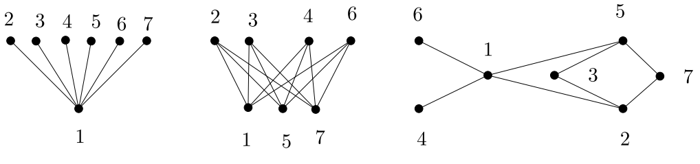
The first class of graphs which are not complete or complete bipartite that we will examine is \(\Gamma(\mathbb{Z}_2\times \mathbb{Z}_2\times \mathbb{Z}_p)\). See Figures 9 (b) and 15 (a) in Section 3 for prime labelings of this graph in the cases of \(p=2\) and \(p=3\).
Theorem 2.9. The zero-divisor graph \(\Gamma(\mathbb{Z}_2\times \mathbb{Z}_2\times \mathbb{Z}_p)\) is prime for all prime numbers \(p\).
Proof. This zero-divisor graph consists of \(3p\) vertices: \(u=(1,1,0), v_i=(0,0,i)\), \(w_1=(0,1,0)\), \(w_2=(1,0,0)\), \(x_i=(1,0,i)\), and \(y_i=(0,1,i)\) where each \(i=1,2,\ldots,p-1\). Edges are of the form \(uv_i\), \(v_iw_j\), \(w_1w_2\), \(w_1x_i\), and \(w_2y_i\) where each \(i\) is from \(1\) to \(p-1\) and \(j=1,2\).
We construct a prime labeling \(\ell: V\rightarrow \{1,2,\ldots, 3p\}\) as follows: first assign \(\ell(w_1)=1\), \(\ell(u)=2\), and \(\ell(w_2)=q\) where \(q\) is a prime with \(\frac{3p}{2}< q\leq 3p\) guaranteed to exist by Bertrand’s Postulate. We next label \(v_1,\ldots, v_{p-1}\) using the sequence of odd integers \(3,5,\ldots 2p-1\). If \(q\leq 2p-1\), replace that label with \(2p+1\). Finally, label the vertices \(x_i\) and \(y_i\) arbitrarily with the remaining unused labels from the labeling set \(\{1,2,\ldots, 3p\}\).
To show that \(\ell\) is a prime labeling, we first consider the edges of the form \(uv_i\). Since \(\ell(u)=2\), this label is relatively prime with the odd labels used on each \(v_i\). For edges \(w_1w_2\), \(w_1v_i\), and \(w_1x_i\), the label \(\ell(w_1)=1\) is clearly relatively prime with all of its adjacent labels. All remaining edges are incident on the vertex \(w_2\). Since \(\ell(w_2)=q\) is a prime larger than \(\frac{3p}{2}\), it is relatively prime with each \(\ell(v_i)\) and \(\ell(y_i)\). Therefore, this is a prime labeling. ◻
The labeling from the previous result can be applied more generally to \(\Gamma(\mathbb{Z}_2\times \mathbb{Z}_2\times \mathbb{F}_{p^n})\) for any finite field \(\mathbb{F}_{p^n}\). This new graph has \(3p^n\) vertices. Assigning \(\ell(u)=2\), \(\ell(w_1)=1\), \(\ell(w_2)=q\) (for a prime \(q>3p^n/2\)), and any odd labels on the vertices \((0,0,c)\) for the nonzero \(c\in\mathbb{F}_{p^n}\) will again result in a prime labeling, giving us the following corollary.
Corollary 2.10. The zero-divisor graph \(\Gamma(\mathbb{Z}_2\times \mathbb{Z}_2\times \mathbb{F}_{p^n})\) is prime for all prime numbers \(p\) and positive integers \(n\).
We next extend the previous result from using \(\mathbb{Z}_2\) as factors within the ring to now use \(\mathbb{Z}_3\).
Theorem 2.11. The zero-divisor graph \(\Gamma(\mathbb{Z}_3\times \mathbb{Z}_3\times \mathbb{Z}_p)\) is prime for all prime numbers \(p\).
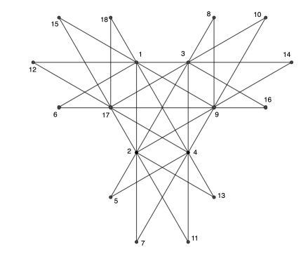
Proof.First observe that the \(p=2\) case is shown to be prime in Figure 23, and see Figure 2 below for when \(p=3\). Then we now assume \(p\geq 5\). This zero-divisor graph consists of \(5p+3\) vertices. They include \(u_1=(0,1,0)\), \(u_2=(0,2,0)\), \(v_1=(1,0,0)\), \(v_2=(2,0,0)\), \(x_1=(1,1,0)\), \(x_2=(1,2,0)\), \(x_3=(2,1,0)\), \(x_4=(2,2,0)\), \(p-1\) vertices of the form \((0,0,c)\), \(2p-2\) vertices of the form \((1,0,c)\) or \((2,0,c)\) for each \(c=1,2,\ldots,p-1\), and \(2p-2\) of the form \((0,1,c)\) or \((0,2,c)\). Edges connect each \(u_i\) to \(v_j\), each vertex \((0,0,c)\) to the \(u_i\) and \(v_j\) vertices, and the following complete bipartite subgraphs where \(c=1,2,\ldots, p-1\):
\(\bullet\) \(K_{2,2p-2}\) connecting \(\{u_1,u_2\}\) and \(\{(1,0,c),(2,0,c)\}\),
\(\bullet\) \(K_{2,2p-2}\) connecting \(\{v_1,v_2\}\) and \(\{(0,1,c),(0,2,c)\}\),
\(\bullet\) \(K_{4,p-1}\) connecting \(\{x_1,x_2,x_3,x_4\}\) and \(\{(0,0,c)\}.\)
As we begin to label \(\Gamma(\mathbb{Z}_3\times \mathbb{Z}_3\times \mathbb{Z}_p)\), note that by Bertrand’s Postulate, there is a prime number \(q_1\) with \(p<q_1\leq 2p\), and likewise another prime \(q_2\) \(\frac{5p+3}{2}<q_2\leq 5p+3\). We first assign the labels \(\ell(u_1)=1\), \(\ell(u_2)=q_2\), \(\ell(v_1)=p\), \(\ell(v_2)=q_1\), \(\ell(x_1)=2\), \(\ell(x_2)=4\), \(\ell(x_3)=8\), and \(\ell(x_4)=16\). Note that we assumed \(p\geq 5\), so \(|V|\geq 28\), allowing the use of the label 16.
Within the set of remaining labels, there are at most 7 numbers with a factor of \(p\) or \(q_1\): \(2p, 3p, 4p, 5p, 2q_1, 3q_1,\) and \(4q_1\). This is since \(|V|=5p+3\) with \(p\geq 5\), so both \(6p\) and \(5q_1\geq 5(p+2)=5p+10\) are too large. We use these labels on a subset of the vertices of the form \((1,0,c)\) and \((2,0,c)\), noting that there are \(2p-2>7\) such vertices. Thus far, we have used either 6 or 7 odd labels, depending on whether \(3q_1\leq 5p+3\). Hence there are at least \(\frac{5p+3}{2}-7\) unused odd labels, which is greater than \(p-1\) for \(p\geq 5\). Then we can label the vertices of the form \((0,0,c)\) for \(c=1,2,\ldots,p-1\) with any of these odd labels. Finally, the remaining labels can be assigned arbitrarily to all \((1,0,c)\) and \((2,0,c)\) that are still unlabeled and to each vertex of the form \((0,1,c)\) and \((0,2,c)\).
To show this is a prime labeling, we first consider edges incident on \(u_1\) or \(u_2\). Since these vertices are labeled by 1 and the prime \(q_2>|V|/2\), these edges satisfy the relatively prime condition. Next, the edges of the complete bipartite subgraph \(K_{4,p-1}\) connect labels that are powers of 2 to odd labels, and hence the pairs of labels share no common factors. Lastly, all other edges are incident on \(v_1=(1,0,0)\) or \(v_2=(2,0,0)\), where recall that \(\ell(v_1)=p\) and \(\ell(v_2)=q_1\). All multiples of these two prime numbers were assigned to vertices of the form \((1,0,c)\) or \((2,0,c)\). These vertices are not adjacent to either \(v_i\), thus resulting in relatively prime labels for all edges involving \(v_i\). This proves that the labeling on \(\Gamma(\mathbb{Z}_3\times \mathbb{Z}_3\times \mathbb{Z}_p)\) is in fact prime. ◻
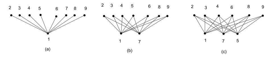
The next three classes of zero-divisor graphs relate to rings of the form \(\mathbb{Z}_p\times \mathbb{Z}_{q^2}\), starting with \(\mathbb{Z}_p\times \mathbb{Z}_4\). For prime labelings of small examples of this class, see in the next section Figure 8 (c) for \(p=2\), Figure 10 (c) for \(p=3\), and Figure 18 (b) for \(p=5\).
Theorem 2.12. The zero-divisor graph \(\Gamma(\mathbb{Z}_p\times \mathbb{Z}_4)\) is prime for all prime numbers \(p\).
Proof. The graph contains a complete bipartite subgraph \(K_{3, p-1}\) connecting the vertices \(\{(0,1),(0,2),(0,3)\}\) (call these \(v_1,v_2,v_3\) respectively) to \(\{(1,0), (2,0),\ldots, (p-1,0)\}\) (call these \(w_1,\ldots, w_{p-1}\)). The vertex \((0,2)\) is also adjacent to \(p-1\) pendant vertices \((1,2),(2,2),\ldots, (p-1,2)\) (call these \(u_1,\ldots, u_{p-1})\). Note that this graph has \(2p+1\) vertices.
Assign labels as follows: \(\ell(v_2)=1\), \(\ell(v_1)=p\), and \(\ell(v_3)=q\) where \(q\) is a prime number such that \(p+1\leq q\leq 2p+1\), which is guaranteed to exist by Bertrand’s Postulate. Then we let \(\ell(u_1)=2p\), \(\ell(u_i)=i\) for \(i=2,\ldots, p-1\), and assign the remaining labels \(\{p+1,\ldots, 2p+1\}-\{q,2p\}\) to the vertices \(w_1,\ldots,w_{p-1}\) arbitrarily.
All edges of the form \(v_2u_i\) and \(v_2w_i\) have \(1\) as the label of an endpoint. The remaining edges \(v_1w_i\) or \(v_3w_i\) have either \(p\) or \(q\) assigned as one of the labels. Since the vertex labelled \(p\) is not adjacent to the one labelled \(2p\), which is the only value up to \(2p+1\) which shares a common factor with \(p\), the edges \(v_1w_i\) have relatively prime labels on the endpoints. Likewise, \(q\) is prime and since \(2q>2p+1\), it is relatively prime with all adjacent labels on the vertices \(w_i\). Thus, the labeling is prime. ◻
A small variation to the labeling for \(\Gamma(\mathbb{Z}_p\times \mathbb{Z}_4)\) allows us to generalize the result to any finite field rather than only \(\mathbb{Z}_p\). Figure 15 (b) displays a prime labeling in the case of the ring \(\mathbb{F}_4\times \mathbb{Z}_4\).
Theorem 2.13. The zero-divisor graph \(\Gamma(\mathbb{F}_{p^n}\times \mathbb{Z}_4)\) is prime for all finite fields \(\mathbb{F}_{p^n}\).
Proof. This zero-divisor graph has the same structure as \(\Gamma(\mathbb{Z}_{p}\times \mathbb{Z}_4)\), but with \(2p^n+1\) vertices: a \(K_{3,p^n-1}\) subgraph, and \(p^n-1\) pendant vertices connected to \((0,2)\). We use a similar labeling beginning with \(\ell(v_1)=1\), \(\ell(v_2)=p\), and \(\ell(v_3)=q\) with \(q\) being a prime such that \(p^n+1\leq q \leq 2p^n+1\). There are only \(\displaystyle \left\lfloor\frac{2p^n+1}{p}\right\rfloor=2p^{n-1}\) multiples of \(p\) in \([1,2p^n+1]\), so \(2p^{n-1}-1\) other than \(p\). We assign these to the \(p^n-1\) pendant vertices that are adjacent only to \(v_2\), which was labeled by 1. Note that \(2p^{n-1}-1\leq p^n-1\) since \(p\geq 2\). Assigning the remaining labels to the \(w_i\) and any unlabeled \(u_i\) vertices results in a prime labeling. ◻
Our next labeling will utilize known results about prime gaps, or the difference between consecutive primes. We denote the \(n\)th prime gap as \(g(p_n)=p_{n+1}-p_n\). As a consequence of the prime number theorem, for any \(\varepsilon>0\), there exists an integer \(N\) such that for all \(n>N\), \(g(p_n)<\varepsilon p_n\). Specific values for \(\varepsilon\) and \(N\) were given by Nagura [15], such as if \(n>9\) or \(p_n\geq 29\), \(g(p_n)<\frac{1}{5}p_n\), or likewise \(p_{n+1}<\frac{6}{5}p_n\).
Theorem 2.14. The zero-divisor graph \(\Gamma(\mathbb{Z}_p\times \mathbb{Z}_9)\) is prime for all primes \(p\).
Proof. Figures 18 (a) and 25 (b) for prime labelings in the cases of \(p=2\) and \(p=3\), respectively, see below in Figure 3 for the case of \(p=5\). Assume \(p\geq 7\).
This zero-divisor graph has \(3p+5\) vertices consisting of two complete bipartite graphs that are adjoined at two vertices. There is \(K_{8,p-1}\) containing vertices \((0,1),(0,2),\ldots, (0,8)\) along with \((1,0),(2,0),\ldots, (p-1,0)\), which we will call \(v_1,\ldots, v_8\) and \(w_1,\ldots, w_{p-1}\). There is also \(K_{2,2p-2}\) which shares the vertices \((0,3)\) and \((0,6)\), or \(v_3\) and \(v_6\), as one set. The other set of \(2p-2\) vertices consists of \((1,3),(2,3),\ldots, (p-1,3),(1,6),(2,6),\ldots, (p-1,6)\), which we refer to as \(u_1,\ldots, u_{2p-2}\).
We will consider the \(7\leq p\leq 23\) cases shortly and will for now assume \(p\geq 29\). If \(p\) is the \(n\)th prime number \(p_n\), by letting \(q_1=p_{n+1}\), we have that \(q_1<\frac{6}{5}p\) according to the prime gap result in [15]. Hence \(2q_1<2(\frac{6}{5})p<3p+5\), so \(2q_1\) is in our labeling set. However since \(q_1\geq p+2\), we have \(3q_1\geq 3(p+2)\geq 3p+6\). Therefore, \(3q_1\) is not one of the labels, and this is also true for any larger primes. Applying Nagura’s result to the prime \(q_1\) implies there is another prime \(q_2=p_{n+2}<\frac{6}{5}q_1<\frac{36}{25}p\) and \(q_3=p_{n+3}<\frac{6}{5}q_2<\frac{216}{125}p\). Finally, we know the next prime \(p_{n+4}<\frac{1296}{625}p<3p\) is also one of the labels in \(\{1,\ldots, 3p+5\}\). For our selection of the prime \(q_4\), though, we will need this prime to also satisfy that \(2q_4>3p+5\). By Bertrand’s Postulate, we know there exists at least one prime in \(\left(\frac{3p+5}{2},3p+5\right]\) which would satisfy that inequality. We let this prime \(p_k\) be \(q_4\) where \(k\geq n+4\).
For the cases of \(p_n=7, 11, 13, 17, 19\), and \(23\), the prime gap result cannot be applied. However, one can verify for these six cases that if you let \(q_1=p_{n+1}, q_2=p_{n+2}, q_3=p_{n+3}\), and \(q_4\) be the largest prime at most \(3p+5\), the necessary inequalities of \(2q_1<3p+5\), \(3q_1>3p+5\), and \(q_4>\frac{3p+5}{2}\) are still true.
We now assign the following labels: \(\ell(v_1)=p\), \(\ell(v_2)=2p\), \(\ell(v_3)=1\), \(\ell(v_4)=q_1\), \(\ell(v_5)=2q_1\), \(\ell(v_6)=q_4\), \(\ell(v_7)=q_2\), and \(\ell(v_8)=q_3\). We then let \(\ell(u_1)=3p\), and assign all remaining \(\frac{3p+5}{2}-2\) even labels on \(u_i\) vertices, of which there are \(2p-3\) as yet unlabeled vertices. Note that since we assumed \(p\geq 7\), we know that \(2p-3\geq \frac{3p+5}{2}-2\). The other \(u_i\) vertices and all \(w_i\) vertices can be labeled with the remaining odd labels arbitrarily.
To show this is a prime labeling, first note that the edges of the form \(v_3u_i\) and \(v_3w_i\) trivially satisfy the relatively prime condition since \(\ell(v_3)=1\). Likewise, the edges \(v_6u_i\) satisfy it as well since \(\ell(v_6)=q_4\), which is a prime larger than \(\frac{|V|}{2}\). For edges \(v_iw_j\) with \(i=1,2,4,5,7\) or \(8\), each of the \(v_i\) vertices are labeled by a prime number, \(2p\), or \(2q_1\). Since all the even labels were assigned to \(u_i\) vertices, none of the labels of \(w_j\) have a factor of \(2\). Since \(3p\) is the label on \(u_1\), there are no other multiples of \(p\) on the labels of any \(w_j\) that would share a common factor with the \(p\) and \(2p\) labels on \(v_1\) and \(v_2\). Finally, the other prime labels \(q_i\) satisfied \(3q_i\geq 3p+6\), so none of the labels \(\ell(w_j)\) are multiples of \(q_i\). Thus, these edges have endpoints labeled with relatively prime integers, making this a prime labeling. ◻

We now will fix the first factor to be \(\mathbb{Z}_2\) and consider rings of the form \(\mathbb{Z}_2\times \mathbb{Z}_{p^2}\). Our prime labeling will require us to estimate how many prime numbers are in our labeling set. For this, we use the prime counting function \(\pi(x)\) to represent the number of primes less than or equal to a real number \(x\). The bounds \(\frac{x}{\ln{x}}<\pi(x)<\frac{1.25506x}{\ln{x}}\) have been shown in [18], where the lower bound is valid for \(x>1\) and the upper bound for \(x\geq 17\). The lower bound will be used in the following proof, while we will utilize both bounds in subsequent results.
Theorem 2.15. The zero-divisor graph \(\Gamma(\mathbb{Z}_{2}\times \mathbb{Z}_{p^2})\) is prime for all prime numbers \(p\).
Proof. See Figures 8(c) and 18(a) for prime labelings of this graph with \(p=2\) and \(p=3\). Assume then that \(p\geq 5\).
This graph has \(p^2+p-1\) vertices, which include \(p^2-1\) of the form \((0,b)\) for \(b=1,2,\ldots,p^2-1\) and \(p\) of the form \((1,kp)\) for \(k=0,1,\ldots, p-1\). The vertex \((1,0)\) is connected by an edge to all \(p^2-1\) vertices \((0,b)\), of which the \(p^2-p\) with \(b\) not being a multiple of \(p\) are degree \(1\). All other edges form a complete bipartite subgraph \(K_{p-1,p-1}\) connecting \(\{(0,kp)\}\) to \(\{(1,kp)\}\) for \(k=1,2,\ldots p-1\).
We first use \(1\) to label the vertex \((1,0)\). Then the only edges that don’t include this vertex are within the \(K_{p-1,p-1}\) subgraph. We claim there are enough prime numbers in the interval \([2,p^2+p-1]\) to use as labels of the \(2p-2\) vertices of this subgraph. When \(p=5\), this is true since there are \(\pi(29)=10>8=2\cdot 5-2\), and likewise for \(p=7\), we have \(\pi(55)=16>12=2\cdot 7-2\).
Now assume \(p\geq 11\). Then since \(p^2\geq 17\), we can use the lower bound for \(\pi(x)\) to show \[\pi(p^2+p-1)>\pi(p^2)>\frac{p^2}{\ln(p^2)}=\frac{p^2}{2\ln{p}}>\frac{p^2}{\frac{1}{2}p}=2p>2p-2,\] where we note \(2\ln{p}<\frac{1}{2}p\) for all \(p\geq 11\). Thus, there are enough prime numbers in our labeling set to label all vertices of the \(K_{p-1,p-1}\) subgraph, resulting in each adjacent pair of labels being relatively prime. Therefore, placing all remaining labels on the \(p^2-p\) degree \(1\) vertices completes a prime labeling. ◻
We conclude this section with a final class of zero-divisor graphs, \(\Gamma(\mathbb{Z}_{p^n})\). Note that the ring \(\mathbb{Z}_{p^n}\) with \(n=1\) has no nonzero zero-divisors, so we only consider \(n\geq 2\). Recall that, by Theorem 2.3 (1) , the graph \(\Gamma(\mathbb{Z}_{p^2})\) is not prime for \(p>3\). We will show that \(\Gamma(\mathbb{Z}_{p^n})\) is prime for all \(n\geq 3\) and all primes \(p\). Examples of these graphs with a prime labeling for \(p^n=2^3\), \(2^4\), and \(3^3\) can be found in Figures 6 (a), 11 (a), and 13 (c), respectively.
The approach we take to prove the general case of \(\mathbb{Z}_{p^n}\) relies on bounds that work best when \(n\geq 4\), so we first consider \(n=3\) separately. The following lemma involving a specific set of complete bipartite graphs will aid in our proof.
Lemma 2.16. The complete bipartite graph \(K_{m,m(m+1)}\) is prime for all positive integers \(m\).
Proof. By Theorem 2.3 (2), (3), and (4), the graphs \(K_{1,2}\), \(K_{2,6}\), and \(K_{3,12}\) are prime, so we assume \(m\geq 4\). By Theorem 2.7, \(K_{m,m(m+1)}\) is prime if \(m(m+1)\geq R_{m-1}-m\), where \(R_{m-1}\) is the \((m-1)\)st Ramanujan prime. Simplifying this inequality, our result will be proven if \(R_{m-1}\leq m^2+2m\).
Sondow [20] proved the upper bound \(R_n<4n \log(4n)\) for all Ramanujan primes with \(n\geq 1\). It follows from this inequality that \[R_{m-1}<4(m-1)\ln(4(m-1))<m^2+2m,\] for all \(m\geq 12\). From the entries of Ramanujan primes in [19], the inequality holds for \(4\leq m\leq 11\) as well, completing the proof. ◻
Theorem 2.17. The zero-divisor graph \(\Gamma(\mathbb{Z}_{p^3})\) is prime for all prime numbers \(p\).
Proof. Two nonzero elements in \(\mathbb{Z}_{p^3}\) have a product of 0 if and only if they are both multiples of \(p\) and at least one is a multiple of \(p^2\). This implies the zero-divisor graph has \(p^2-1\) vertices corresponding to all nonzero multiples of \(p\). Additionally, all edges \(uv\) must have one or both of \(u\) and \(v\) be a multiple of \(p^2\).
The graph \(\Gamma(\mathbb{Z}_{p^3})\) thus contains a complete subgraph \(K_{p-1}\) on the vertices \(p^2, 2p^2,\ldots, (p-1)p^2\). All other edges are within a complete bipartite spanning subgraph \(K_{p-1,(p-1)p}\), where the \((p-1)p\) vertices are the elements with \(p\) as a factor, but not \(p^2\).
By Lemma 2.16, \(K_{p-1,(p-1)p}\) is prime for all prime numbers \(p\). This result is based on Theorem 2.7, whose condition on the size of \(n=p(p+1)\) compared to the Ramanujan prime \(R_{p-2}\) implies there are at least \(p-2\) primes in the labeling set that are greater than \(\displaystyle\frac{|V|}{2}\). These primes, along with the label 1, are assigned as labels of the \(p-1\) vertices on the smaller side of the bipartition. Therefore, applying this labeling to \(\Gamma(\mathbb{Z}_{p^3})\) would not only cause the edges in the complete bipartite spanning subgraph to have relatively prime labels on their endpoints, but also the \(1\) and prime numbers have no common factors within the complete subgraph \(K_{p-1}\). Thus, we have a prime labeling for \(\Gamma(\mathbb{Z}_{p^3})\). ◻
We now extend the previous result to be true for the ring \(\mathbb{Z}_{p^n}\) for higher powers of \(n\).
Theorem 2.18. The zero-divisor graph \(\Gamma(\mathbb{Z}_{p^n})\) is prime for all prime numbers \(p\) and positive integers \(n\geq 4\).
Proof. This zero-divisor graph consists of \(p^{n-1}-1\) vertices corresponding to all nonzero multiples of \(p\) in \(\mathbb{Z}_{p^n}\). We can group the vertices as follows based on the highest power of \(p\) that divides each element. We define \(V_i:=\{a\in Z_{p^n} \mid \text{ gcd} (a, p^n)=p^i \text{ for } 1\leq i \leq n-1\}\). There are \(p-1\) such \(a\in \mathbb{Z}_{p^n}\) with gcd\((a, p^n)=p^{n-1}\), \((p-1)p\) with gcd\((a, p^n)=p^{n-2}\), \((p-1)p^2\) with gcd\((a, p^n)=p^{n-3}, \ldots, (p-1)p^{n-3}\) with gcd\((a, p^n)=p^2\), and \((p-1)p^{n-2}\) with gcd\((a, p^n)=p\). Hence we have \(|V_i|=(p-1)p^{n-i-1}\).
Pairs of zero-divisors in \(\mathbb{Z}_{p^n}\) can only multiply to be zero if the total number of factors of \(p\) between the pair is at least \(n\). Therefore, all vertices in \(V_i\) are adjacent to every vertex in \(V_j\) for any pair \(i,j\in \{1,\ldots, n-1\}\) such that \(i+j\geq n\).
We now consider cases based on the parity of \(n\). First assume that \(n\) is odd. This means that all \(u\in V_i\) and \(v\in V_j\) are adjacent to each other if \(i,j\geq (n+1)/2\), or in other words, there is an induced complete subgraph on \(V_{\frac{n+1}{2}}\cup \cdots \cup V_{n-1}\). We observe that there is no edge between any pair \(u,v\in V_1\cup \cdots \cup V_{\frac{n-1}{2}}\), implying all edges include a vertex in \(V_{\frac{n+1}{2}}\cup \cdots \cup V_{n-1}\). Thus, every pair of adjacent labels will be relatively prime if we can label the vertices in this set using \(1\) and prime numbers that are greater than \(\displaystyle \frac{|V|}{2}=\frac{p^{n-1}-1}{2}.\)
Enumerating the size of this collection of vertices, we see that \[|V_{\frac{n+1}{2}}\cup \cdots \cup V_{n-1}|=\sum_{i=\frac{n+1}{2}}^{n-1} (p-1)p^{n-i-1}=\sum_{j=0}^{\frac{n-3}{2}} (p-1)p^j=\frac{(p-1)(1-p^{\frac{n-1}{2}})}{1-p}=p^{\frac{n-1}{2}}-1.\] Then our result follows if we can show the interval \(\displaystyle\left(\frac{p^{n-1}-1}{2},p^{n-1}-1\right]\) contains at least \(p^{\frac{n-1}{2}}-2\) primes to use alongside the label 1. To simplify this claim, we will ignore the subtractions by 1, which we can do since \(p^{n-1}\) is not prime and not even. We also let \(m=n-1\) so that our goal is to prove that \(\displaystyle\left[\frac{p^{m}}{2},p^m\right]\) contains at least \(p^{m/2}-2\) prime numbers. Note that by our previous assumption, \(m\) is even and \(m\geq 4\).
We will use the inequalities for \(\pi(x)\) from [18] mentioned above to estimate \(\pi(p^m)-\pi(p^m/2)\). Given our assumptions on \(p\) and \(n\), the only input that doesn’t meet the necessary condition of \(\frac{p^m}{2}\geq 17\) is \(p=2\) and \(m=4\), which we will address shortly. Applying these bounds gives us \[\begin{aligned} \pi(p^m)-\pi(p^m/2)&>\frac{p^m}{\ln{p^m}}-\frac{1.25506\cdot p^m/2}{\ln{(p^m/2)}}\\ &\geq\frac{p^m}{\ln{p^m}}-\frac{.62753 p^{m}}{\ln{p^{m-1}}}\\ &=\frac{p^m}{m\ln{p}}-\frac{.62753 p^{m}}{(m-1)\ln{p}}\\ &=\frac{(m-1) p^m-.62753mp^m}{m(m-1)\ln{p}}\\ &=\frac{(.37247m-1) p^m}{m(m-1)\ln{p}}\\ &\geq \frac{.12mp^m}{m(m-1)\ln{p}} (\text{since }m\geq 4)\\ &=\frac{.12p^m}{(m-1)\ln{p}} \\ &=\frac{p^m}{\frac{(m-1)\ln{p}}{.12}}. \end{aligned}\]
Considering the denominator on the last line, one can verify that \(\frac{(m-1)\ln{p}}{.12}<p^{m/2}\) for all \(p\geq 7\) when \(m=4\), for all \(p\geq 5\) when \(m=6\), for all \(p\geq 3\) when \(m= 8\) or \(10\), and for all primes \(p\) when \(m\geq 12\). Therefore, as long as \(m\) and \(p\) meet the described requirements, we have \[\pi(p^m)-\pi(p^m/2)>\frac{p^m}{\frac{(m-1)\ln{p}}{.12}}>\frac{p^m}{p^{m/2}}=p^{m/2}>p^{m/2}-2.\]
Thus, we see there are enough prime numbers in the interval so that at least one vertex on each edge is labelled by a prime number that is relatively prime to all other labels, creating a prime labeling. The remaining cases of small pairs of \(n\) and \(p\) are \(p=2\) with \(n=5, 7, 9,\) or \(11\) (note this includes the aforementioned case where the \(\pi(x)\) input was less than 17), \(p=3\) with \(n=5\) or \(7\), and \(p=5\) with \(n=5\). Even though our \(\pi(x)\) estimations did not directly show there were enough prime numbers in the interval, the required number of primes are in fact present as seen by the following:
\(p=2\), \(n=5\): \(\pi(15)-\pi(8)=2=2^2-2\),
\(p=2\), \(n=7\): \(\pi(63)-\pi(32)=7>6=2^3-2\),
\(p=2\), \(n=9\): \(\pi(255)-\pi(128)=23>14=2^4-2\),
\(p=2\), \(n=11\): \(\pi(1023)-\pi(512)=75>30=2^5-2\),
\(p=3\), \(n=5\): \(\pi(80)-\pi(40)=10>7=3^2-2\),
\(p=3\), \(n=7\): \(\pi(728)-\pi(364)=57>25=3^3-2\),
\(p=5\), \(n=5\): \(\pi(624)-\pi(312)=50>23=5^2-2.\)
This concludes the case of \(\Gamma(\mathbb{Z}_{p^n})\) being prime for all odd \(n\geq 5\).
We now assume that \(n\) is even and that \(n\geq 4\). We again consider the same grouping of the vertices into sets \(V_i\) as in the odd case. Vertices in \(V_i\) remain adjacent to vertices in \(V_j\) if \(i+j\geq n\). However, all vertex pairs \(u\in V_i\) and \(v\in V_j\) are now adjacent if \(i,j\geq \frac{n}{2}\). We also have that all edges must be incident on a vertex in \(V_{\frac{n}{2}}\cup \cdots \cup V_{n-1}\).
Observe that \(V_{n/2}\) is a complete subgraph with \(|V_{n/2}|=(p-1)p^{n/2-1}\) where its vertices are only adjacent to \(v\in V_i\) with \(i\geq n/2\). Hence we can use smaller primes, i.e., ones that are less than \(\frac{|V|}{2}\), to label \(V_{n/2}\) and reserve larger primes for the sets with \(i>n/2\). We claim there are at least \((p-1)p^{n/2-1}\) primes in \(\left[1,\frac{p^{n-1}-1}{2}\right]\) to assign to vertices in \(V_{n/2}\). Letting \(m=n-1\), we need at least \((p-1)p^{(m-1)/2}\) prime numbers in that interval. Using the lower bound for \(\pi(x)\), we have \[\begin{aligned} \pi\left(\frac{p^{n-1}-1}{2}\right)&=\pi\left(\frac{p^m-1}{2}\right)\\ &=\pi\left(\frac{p^m}{2}\right)\\ &>\frac{p^m/2}{\ln(p^m/2)}\\ &\geq \frac{p^m/2}{\ln(p^{m-1})}\\ &=\frac{p^m}{2(m-1)\ln{p}}.\\ \end{aligned}\]
We can verify that \(2(m-1)\ln{p}<p^{\frac{m-1}{2}}\) for \(p\geq 11\) when \(m=3\), for \(p\geq 3\) when \(m=5\) or \(7\), and for all primes \(p\) when \(m\geq 9\). We will consider the remaining small cases later in the proof, but for \(m\) and \(p\) satisfying this inequality, we then have
\[\pi\left(\frac{p^{n-1}-1}{2}\right)>\frac{p^m}{p^{(m-1)/2}}= p^{\frac{m+1}{2}}=p\cdot p^{\frac{m-1}{2}}>(p-1) p^{\frac{m-1}{2}}.\]
We now focus on labeling the vertices of \(V_{\frac{n+2}{2}}\cup \cdots \cup V_{n-1}\) with larger prime numbers. This collection of vertices has the following cardinality: \[|V_{\frac{n+2}{2}}\cup \cdots \cup V_{n-1}|=\sum_{i=\frac{n+2}{2}}^{n-1} (p-1)p^{n-i-1}=\sum_{j=0}^{\frac{n-4}{2}} (p-1)p^j=\frac{(p-1)(1-p^{\frac{n-2}{2}})}{1-p}=p^{\frac{n-2}{2}}-1.\]
Thus, we can create a prime labeling using 1 and prime numbers that are greater than \(\frac{|V|}{2}\) on these \(p^{\frac{n-2}{2}}-1\) vertices. Hence we need to show that there are at least \(p^{\frac{n-2}{2}}-2\) prime numbers in the interval \(\left(\frac{p^{n-1}-1}{2},p^{n-1}-1\right]\). Using the same \(m=n-1\) substitution where \(m\) is odd and at least 3, we need \(p^{\frac{m-1}{2}}-2\) primes in \(\left(\frac{p^{m}-1}{2},p^{m}-1\right]\), or in the simpler interval \(\left[\frac{p^{m}}{2},p^{m}\right]\) since we know \(p^m\) is not prime.
Using the prime counting function estimates and noting that the input into \(\pi(x)\) is at least 17 in all cases but a soon to be considered case of \(p=2\) with \(m=3\), we have \[\begin{aligned} \pi(p^m)-\pi(p^m/2)&>\frac{p^m}{\ln{p^m}}-\frac{1.25506\cdot p^m/2}{\ln{(p^m/2)}}\\ &\geq\frac{(.37247m-1) p^m}{m(m-1)\ln{p}}\\ &\geq \frac{.039mp^m}{m(m-1)\ln{p}} (\text{since }m\geq 3)\\ &=\frac{.039p^m}{(m-1)\ln{p}} \\ &=\frac{p^m}{\frac{(m-1)\ln{p}}{.039}}. \end{aligned}\]
Considering the final denominator, one can verify \(\frac{(m-1)\ln{p}}{.039}<p^{\frac{m+1}{2}}\) for all \(p\geq 13\) when \(m=3\), for all \(p\geq 7\) when \(m=5\), for all \(p\geq 5\) when \(m= 7\), for all \(p\geq 3\) when \(m=9\), \(11\), or \(13\), and for all prime numbers when \(m\geq 15\). Therefore, as long as \(m\) and \(p\) meet the criteria above, we have \[\pi(p^m)-\pi(p^m/2)>\frac{p^m}{\frac{(m-1)\ln{p}}{.039}}>\frac{p^m}{p^{\frac{m+1}{2}}}=p^{\frac{m-1}{2}}>p^{\frac{m-1}{2}}-2.\]
Thus, for all but a handful of remaining cases of small \(n\) and \(p\), we can create a prime labeling in the even case. This is true since every edge is incident on a vertex labeled by either a prime that is greater than \(\frac{|V|}{2}\) or by two prime numbers below \(\frac{|V|}{2}\).
There are thirteen remaining pairs of \(n\) and \(p\) that failed to meet one or more of the criteria within the proof for the even case. These are \(p=2\) with \(n=4,6,8,10,12,\) and \(14\), \(p=3\) with \(n=4,6\), and \(8\), \(p=5\) with \(n=4\) and \(6\), \(p=7\) with \(n=4\), and \(p=11\) with \(n=4\). The following table shows that in eleven of the cases, both of the intervals do include the necessary number of prime numbers, where a blank entry is a situation where our \(\pi(x)\) arguments already covered that case.
| \(p\) | \(n\) | \(\pi\left(\frac{p^{n-1}-1}{2}\right)\) | \((p-1)p^{n/2-1}\) | \(\pi(p^{n-1}-1)-\pi\left(\frac{p^{n-1}-1}{2}\right)\) | \(p^{\frac{n-2}{2}}-2\) |
|---|---|---|---|---|---|
| 2 | 4 | 2 | 2 | 2 | 0 |
| 2 | 6 | 6 | 4 | 5 | 2 |
| 2 | 8 | 18 | 8 | 13 | 6 |
| 2 | 10 | 43 | 14 | ||
| 2 | 12 | 137 | 30 | ||
| 2 | 14 | 464 | 62 | ||
| 3 | 4 | 6 | 6 | 3 | 1 |
| 3 | 6 | 23 | 7 | ||
| 3 | 8 | 144 | 25 | ||
| 5 | 4 | 18 | 20 | 12 | 3 |
| 5 | 6 | 199 | 23 | ||
| 7 | 4 | 39 | 42 | 29 | 5 |
| 11 | 4 | 96 | 9 |
Observe that in the two cases of \(p=5\), \(n=4\) and \(p=7\), \(n=4\) there are not enough small primes for the vertices in \(V_2\). However, there are enough large primes that \(V_3\) can be labeled and have additional large primes remaining to cover the rest of \(V_2\).
This concludes even \(n\) case, proving that \(\Gamma(\mathbb{Z}_{p^n})\) is prime for all prime numbers \(p\) and any \(n\geq 4\). ◻
In this section, we look at zero-divisor graphs with up to 14 vertices to classify which graphs admit prime labelings. The list of graphs to examine are due to work by Redmond [16, 17]. Again, we know every finite zero-divisor graph is connected, so we know they are all vertex prime, so we only determine which ones are prime.
Graphs with \(|V|=1\)
| \(R\) | \(\Gamma(R)\) | Prime? |
|---|---|---|
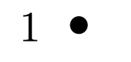
| \(\mathbb{Z}_4\) | \(K_1\) | Yes – Fig. 4 |
| \(\mathbb{Z}_2[X]/(X^2)\) | \(K_1\) | Yes – Fig. 4 |
Graphs with \(|V|=2\)
| \(R\) | \(\Gamma(R)\) | Prime? |
|---|---|---|
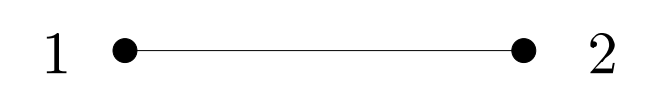
| \(\mathbb{Z}_9\) | \(K_2\) | Yes – Fig. 5 |
| \(\mathbb{Z}_2\times \mathbb{Z}_2\) | \(K_2\) | Yes – Fig. 5 |
| \(\mathbb{Z}_3[X]/(X^2)\) | \(K_2\) | Yes – Fig. 5 |
Graphs with \(|V|=3\)
| \(R\) | \(\Gamma(R)\) | Prime? |
|---|---|---|
| \(\mathbb{Z}_6\) | \(K_{1,2}\) | Yes – Fig. 6 (a) |
| \(\mathbb{Z}_8\) | \(K_{1,2}\) | Yes – Fig. 6 (a) |
| \(\mathbb{Z}_2[X]/(X^3)\) | \(K_{1,2}\) | Yes – Fig. 6 (a) |
| \(\mathbb{Z}_4[X]/(2X,X^2-2)\) | \(K_{1,2}\) | Yes – Fig. 6 (a) |
| \(\mathbb{Z}_2[X,Y]/(X,Y)^2\) | \(K_{3}\) | Yes – Fig. 6 (b) |
| \(\mathbb{Z}_4[X]/(2,X)^2\) | \(K_{3}\) | Yes – Fig. 6 (b) |
| \(\mathbb{F}_4[X]/(X^2)\) | \(K_{3}\) | Yes – Fig. 6 (b) |
| \(\mathbb{Z}_4[X]/(X^2+X+1)\) | \(K_{3}\) | Yes – Fig. 6 (b) |
Graphs with \(|V|=4\)
| \(R\) | \(\Gamma(R)\) | Prime? |
|---|---|---|
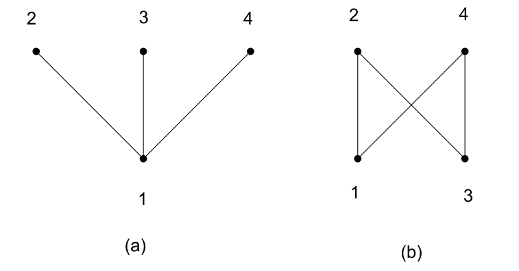
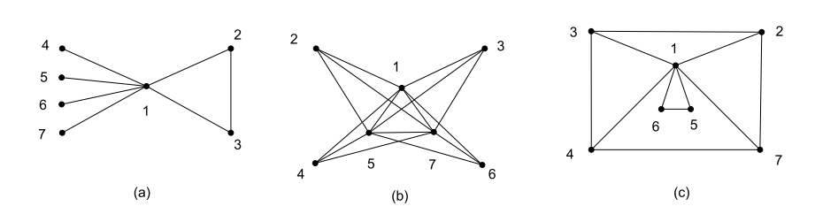
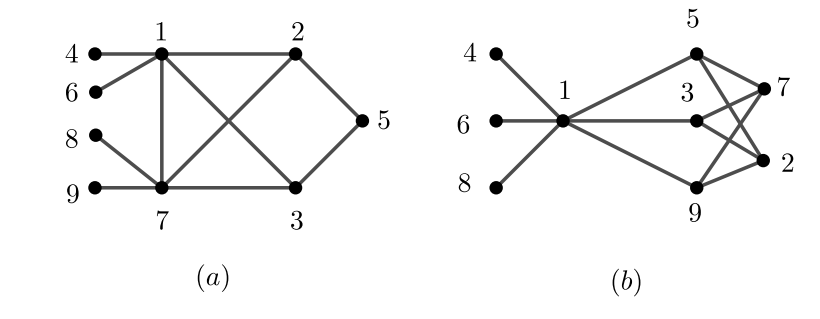
| \(\mathbb{Z}_2\times \mathbb{F}_4\) | \(K_{1,3}\) | Yes – 7 (a) |
| \(\mathbb{Z}_3 \times \mathbb{Z}_3\) | \(K_{2,2}\) | Yes – 7 (b) |
| \(\mathbb{Z}_{25}\) | \(K_{4}\) | No – Thm 2.3 (1) |
| \(\mathbb{Z}_5[X]/(X^2)\) | \(K_{4}\) | No – Thm 2.3 (1) |
Graphs with \(|V|=5\)
| \(R\) | \(\Gamma(R)\) | Prime? |
|---|---|---|
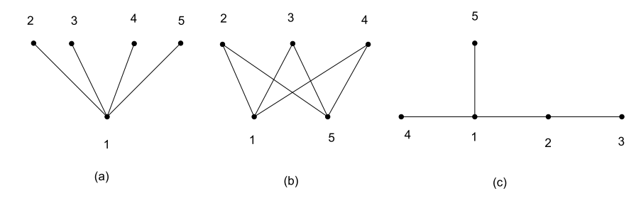
| \(\mathbb{Z}_2\times \mathbb{Z}_5\) | \(K_{1,4}\) | Yes – Fig. 8 (a) |
| \(\mathbb{Z}_3 \times \mathbb{F}_4\) | \(K_{2,3}\) | Yes – Fig. 8 (b) |
| \(\mathbb{Z}_{2}\times \mathbb{Z}_{4}\) | Fig. 8 (c) | Yes – Fig. 8 (c) |
| \(\mathbb{Z}_{2}\times \mathbb{Z}_{2}[X]/(X^2)\) | Fig. 8 (c) | Yes – Fig. 8 (c) |
Graphs with \(|V|=6\)
| \(R\) | \(\Gamma(R)\) | Prime? |
|---|---|---|
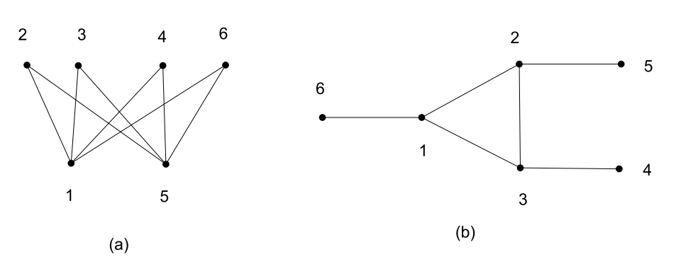
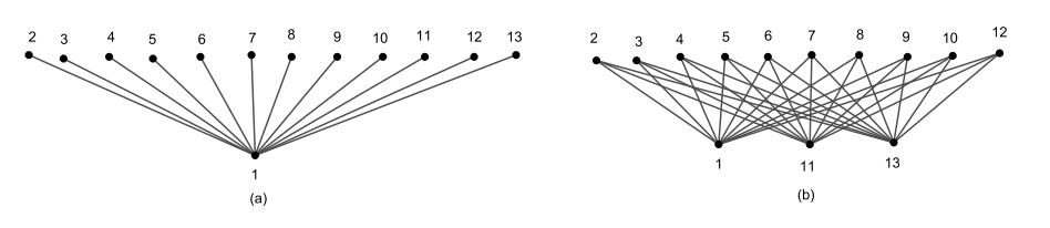
| \(\mathbb{Z}_3\times \mathbb{Z}_5\) | \(K_{2,4}\) | Yes – Fig. 9 (a) |
| \(\mathbb{F}_4 \times \mathbb{F}_4\) | \(K_{3,3}\) | No – Thm 2.3 (4) |
| \(\mathbb{Z}_{49}\) | \(K_6\) | No – Thm 2.3 (1) |
| \(\mathbb{Z}_{7}[X]/(X^2)\) | \(K_6\) | No – Thm 2.3 (1) |
| \(\mathbb{Z}_{2}\times \mathbb{Z}_{2}\times \mathbb{Z}_2\) | Fig. 9 (b) | Yes – Fig. 9 (b) |
Graphs with \(|V|=7\)
| \(R\) | \(\Gamma(R)\) | Prime? |
|---|---|---|
| \(\mathbb{Z}_2\times \mathbb{Z}_7\) | \(K_{1,6}\) | Yes – Fig. 10 (a) |
| \(\mathbb{F}_4 \times \mathbb{Z}_5\) | \(K_{3,4}\) | Yes – Fig. 10 (b) |
| \(\mathbb{Z}_3 \times \mathbb{Z}_4\) | Fig. 10 (c) | Yes – Fig. 10 (c) |
| \(\mathbb{Z}_{3}\times \frac{\mathbb{Z}_2[X]}{(X^2)}\) | Fig. 10 (c) | Yes – Fig. 10 (c) |
| \(\mathbb{Z}_{16}\) | Fig. 11 (a) | Yes – Fig. 11 (a) |
| \(\frac{\mathbb{Z}_2[X]}{(X^4)}\) | Fig. 11 (a) | Yes – Fig. 11 (a) |
| \(\frac{\mathbb{Z}_4[X]}{(X^2+2)}\) | Fig. 11 (a) | Yes – Fig. 11 (a) |
| \(\frac{\mathbb{Z}_4[X]}{(X^2 +2X + 2)}\) | Fig. 11 (a) | Yes – Fig. 11 (a) |
| \(\frac{\mathbb{Z}_4[X]}{(X^3-2, 2X^2, 2X)}\) | Fig. 11 (a) | Yes – Fig. 11 (a) |
| \(\frac{\mathbb{Z}_{2}[X,Y]}{(X^3, XY, Y^2)}\) | Fig. 11 (b) | Yes – Fig. 11 (b) |
| \(\frac{\mathbb{Z}_{8}[X]}{(2X,X^2)}\) | Fig. 11 (b) | Yes – Fig. 11 (b) |
| \(\frac{\mathbb{Z}_{4}[X]}{(X^3, 2X^2, 2X)}\) | Fig. 11 (b) | Yes – Fig. 11 (b) |
| \(\frac{\mathbb{Z}_{4}[X,Y]}{(X^2-2, XY, Y^2, 2X, 2Y)}\) | Fig. 11 (b) | Yes – Fig. 11 (b) |
| \(\frac{\mathbb{Z}_{4}[X]}{(X^2+2X)}\) | Fig. 11 (c) | Yes – Fig. 11 (c) |
| \(\frac{\mathbb{Z}_{8}[X]}{(2X, X^2+4)}\) | Fig. 11 (c) | Yes – Fig. 11 (c) |
| \(\frac{\mathbb{Z}_{2}[X,Y]}{(X^2, Y^2-XY)}\) | Fig. 11 (c) | Yes – Fig. 11 (c) |
| \(\frac{\mathbb{Z}_{4}[X,Y]}{(X^2, Y^2-XY, XY-2, 2X, 2Y)}\) | Fig. 11 (c) | Yes – Fig. 11 (c) |
| \(\frac{\mathbb{Z}_{4}[X,Y]}{(X^2, Y^2, XY-2, 2X, 2Y)}\) | Fig. 12 | Yes – Fig. 12 |
| \(\frac{\mathbb{Z}_{2}[X,Y]}{(X^2, Y^2)}\) | Fig. 12 | Yes – Fig. 12 |
| \(\frac{\mathbb{Z}_{4}[X]}{(X^2)}\) | Fig. 12 | Yes – Fig. 12 |
| \(\frac{\mathbb{Z}_{2}[X,Y,Z]}{(X, Y, Z)^2}\) | \(K_7\) | No – Thm 2.3 (1) |
| \(\frac{\mathbb{Z}_{4}[X,Y]}{(X^2, Y^2, XY, 2X, 2Y)}\) | \(K_7\) | No – Thm 2.3 (1) |
| \(\frac{\mathbb{F}_8[X]}{(X^2)}\) | \(K_7\) | No – Thm 2.3 (1) |
| \(\frac{\mathbb{Z}_4[X]}{(X^3+X + 1)}\) | \(K_7\) | No – Thm 2.3 (1) |
Graphs with \(|V|=8\)
| \(R\) | \(\Gamma(R)\) | Prime? |
|---|---|---|
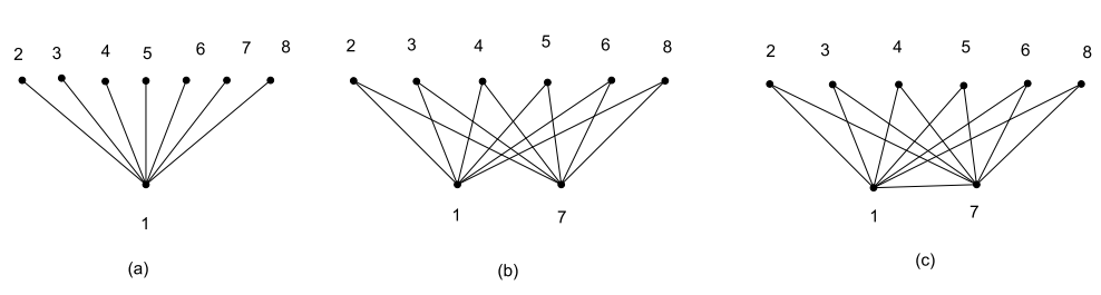
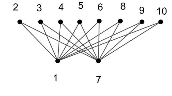
| \(\mathbb{Z}_2\times \mathbb{F}_8\) | \(K_{1,7}\) | Yes – Fig. 13 (a) |
| \(\mathbb{Z}_3 \times \mathbb{Z}_7\) | \(K_{2,6}\) | Yes – Fig. 13 (b) |
| \(\mathbb{Z}_5 \times \mathbb{Z}_5\) | \(K_{4,4}\) | No [8] |
| \(\mathbb{Z}_{27}\) | Fig. 13 (c) | Yes – Fig. 13 (c) |
| \(\frac{\mathbb{Z}_{9}[X]}{(3X,X^2-3)}\) | Fig. 13 (c) | Yes – Fig. 13 (c) |
| \(\frac{\mathbb{Z}_{9}[X]}{(3X,X^2-6)}\) | Fig. 13 (c) | Yes – Fig. 13 (c) |
| \(\frac{\mathbb{Z}_{3}[X]}{(X^3)}\) | Fig. 13 (c) | Yes – Fig. 13 (c) |
| \(\frac{\mathbb{Z}_{3}[X,Y]}{(X,Y)^2}\) | \(K_8\) | No – Thm 2.3 (1) |
| \(\frac{\mathbb{Z}_{9}[X,Y]}{(3,X)^2}\) | \(K_8\) | No – Thm 2.3 (1) |
| \(\frac{\mathbb{F}_{9}[X]}{(X^2)}\) | \(K_8\) | No – Thm 2.3 (1) |
| \(\frac{\mathbb{Z}_{9}[X]}{(X^2+1)}\) | \(K_8\) | No – Thm 2.3 (1) |
Graphs with \(|V|=9\)
| \(R\) | \(\Gamma(R)\) | Prime? |
|---|---|---|
| \(\mathbb{Z}_2\times \mathbb{F}_9\) | \(K_{1,8}\) | Yes – Fig. 14 (a) |
| \(\mathbb{Z}_3 \times \mathbb{F}_8\) | \(K_{2,7}\) | Yes – Fig. 14 (b) |
| \(\mathbb{F}_4\times \mathbb{Z}_{7}\) | \(K_{3,6}\) | Yes – Fig. 14 (c) |
| \(\mathbb{Z}_{2}\times \mathbb{Z}_2 \times \mathbb{Z}_3\) | Fig. 15 (a) | Yes – Fig. 15 (a) |
| \(\mathbb{Z}_4 \times \mathbb{F}_4\) | Fig. 15 (b) | Yes – Fig. 15 (b) |
| \(\frac{\mathbb{Z}_{2}[X]}{(X^2)}\times \mathbb{F}_4\) | Fig. 15 (b) | Yes – Fig. 15 (b) |
Graphs with \(|V|=10\)
| \(R\) | \(\Gamma(R)\) | Prime? |
|---|---|---|
| \(\mathbb{Z}_3\times \mathbb{F}_9\) | \(K_{2,8}\) | Yes – Fig. 16 |
| \(\mathbb{F}_4 \times \mathbb{F}_8\) | \(K_{3,7}\) | No – Thm 2.3 (4) |
| \(\mathbb{Z}_{5}\times \mathbb{Z}_{7}\) | \(K_{4,6}\) | No [8] |
| \(\mathbb{Z}_{121}\) | \(K_{10}\) | No – Thm 2.3 (1) |
| \(\mathbb{Z}_{11}[X]/(X^2)\) | \(K_{10}\) | No – Thm 2.3 (1) |
Graphs with \(|V|=11\)
| \(R\) | \(\Gamma(R)\) | Prime? |
|---|---|---|
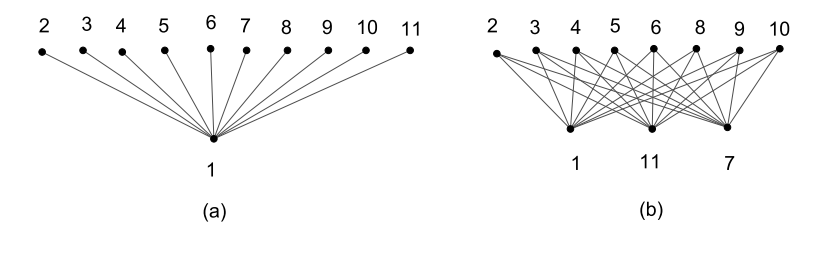
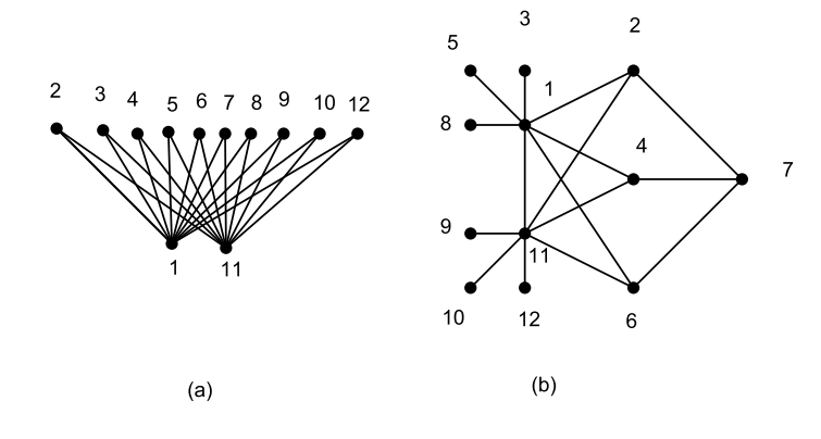
| \(\mathbb{Z}_2\times \mathbb{Z}_{11}\) | \(K_{1,10}\) | Yes – Fig. 17 (a) |
| \(\mathbb{F}_4\times \mathbb{F}_9\) | \(K_{3,8}\) | Yes – Fig. 17 (b) |
| \(\mathbb{Z}_5\times \mathbb{F}_8\) | \(K_{4,7}\) | No – [8] |
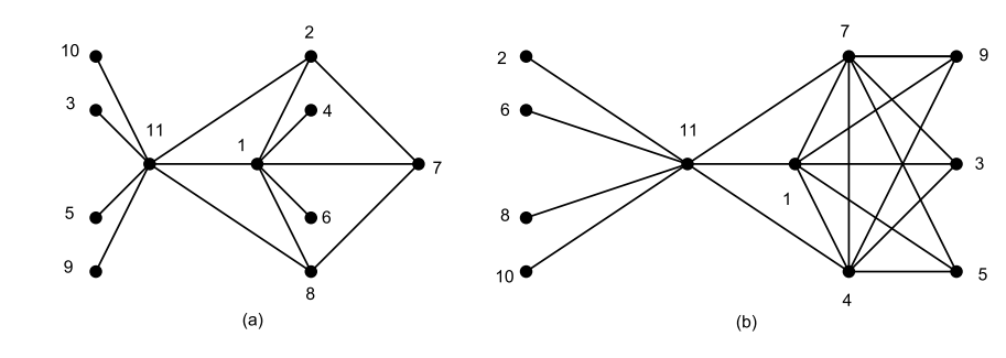
| \(\mathbb{Z}_2\times \mathbb{Z}_9\) | Fig. 18(a) | Yes – Fig. 18 (a) |
| \(\mathbb{Z}_2 \times \mathbb{Z}_{3}[X]/(X^2)\) | Fig. 18(a) | Yes – Fig. 18(a) |
| \(\mathbb{Z}_5 \times \mathbb{Z}_{4}\) | Fig. 18(b) | Yes – Fig. 18(b) |
| \(\mathbb{Z}_5 \times \mathbb{Z}_{2}[X]/(X^2)\) | Fig. 18(b) | Yes – Fig. 18(b) |
| \(\mathbb{Z}_2 \times \mathbb{Z}_{8}\) | Fig. 19 (a) | Yes – Fig. 19 (a) |
| \(\mathbb{Z}_2 \times \mathbb{Z}_{2}[X]/(X^3)\) | Fig. 19 (a) | Yes – Fig. 19 (a) |
| \(\mathbb{Z}_2 \times \mathbb{Z}_{4}[X]/(2X,X^2-2)\) | Fig. 19 (a) | Yes – Fig.19 (a) |
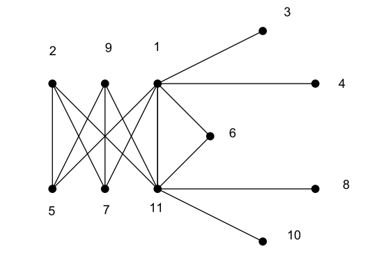
| \(\mathbb{Z}_2 \times \mathbb{Z}_{2}[X,Y]/(X,Y)^2\) | Fig. 19 (b) | Yes – Fig. 19 (b) |
| \(\mathbb{Z}_2 \times \mathbb{Z}_{4}[X]/(2,X)^2\) | Fig. 19 (b) | Yes – Fig. 19 (b) |
| \(\mathbb{Z}_4 \times \mathbb{Z}_{4}\) | Fig. 20 | Yes – Fig. 20 |
| \(\mathbb{Z}_4 \times \mathbb{Z}_{2}[X]/(X^2)\) | Fig. 20 | Yes – Fig. 20 |
| \(\mathbb{Z}_2[X]/(X^2) \times \mathbb{Z}_{2}[X]/(X^2)\) | Fig. 20 | Yes – Fig. 20 |
Graphs with \(|V|=12\)
| \(R\) | \(\Gamma(R)\) | Prime? |
|---|---|---|
| \(\mathbb{Z}_3\times \mathbb{Z}_{11}\) | \(K_{2,10}\) | Yes – Fig. 21 (a) |
| \(\mathbb{Z}_5\times \mathbb{F}_9\) | \(K_{4,8}\) | No – [8] |
| \(\mathbb{Z}_7\times \mathbb{Z}_7\) | \(K_{6,6}\) | No – [8] |
| \(\mathbb{Z}_2\times \mathbb{Z}_2 \times \mathbb{F}_4\) | Fig. 21 (b) | Yes – Fig. 21 (b) |
| \(\mathbb{Z}_{169}\) | \(K_{12}\) | No – Thm 2.3 (1) |
| \(\mathbb{Z}_{13}[X]/(X^2)\) | \(K_{12}\) | No – Thm 2.3 (1) |
Graphs with \(|V|=13\)
| \(R\) | \(\Gamma(R)\) | Prime? |
|---|---|---|
| \(\mathbb{Z}_2\times \mathbb{Z}_{13}\) | \(K_{1,12}\) | Yes – Fig. 22 (a) |
| \(\mathbb{F}_4\times \mathbb{Z}_{11}\) | \(K_{3,10}\) | Yes – Fig. 22 (b) |
| \(\mathbb{Z}_7\times \mathbb{F}_{8}\) | \(K_{6,7}\) | No – [8] |
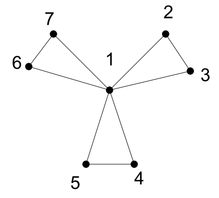
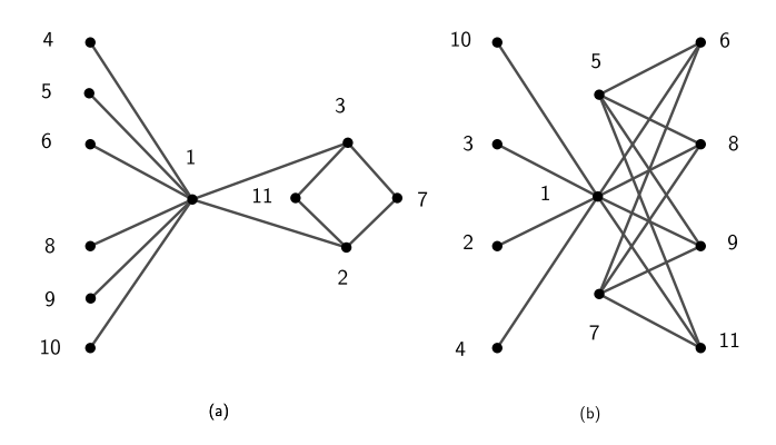
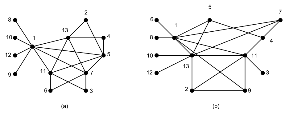
| \(\mathbb{Z}_2\times \mathbb{Z}_3\times \mathbb{Z}_3\) | Fig. 23 (a) | Yes – Fig. 23 (a) |
| \(\mathbb{Z}_2\times \mathbb{Z}_2\times \mathbb{Z}_4\) | Fig. 23 (b) | Yes – Fig. 23 (b) |
| \(\mathbb{Z}_2\times \mathbb{Z}_2\times \mathbb{Z}_2[X]/(X^2)\) | Fig. 23 (b) | Yes – Fig. 23 (b) |
Graphs with \(|V|=14\)
| \(R\) | \(\Gamma(R)\) | Prime? |
|---|---|---|
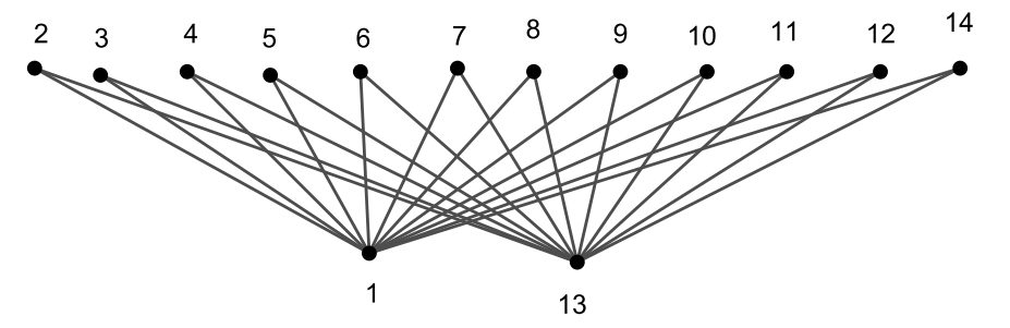
| \(\mathbb{Z}_3\times \mathbb{Z}_{13}\) | \(K_{2,12}\) | Yes – Fig. 24 |
| \(\mathbb{Z}_5\times \mathbb{Z}_{11}\) | \(K_{4,10}\) | No – [8] |
| \(\mathbb{Z}_7\times \mathbb{F}_{9}\) | \(K_{6,8}\) | No – [8] |
| \(\mathbb{F}_8\times \mathbb{F}_8\) | \(K_{7,7}\) | No – [8] |
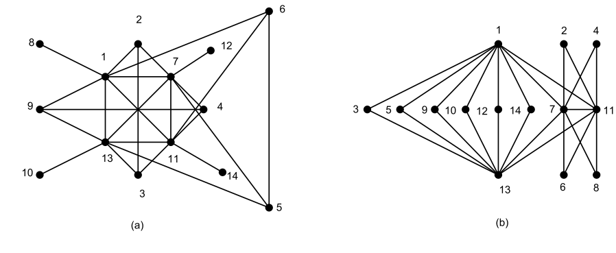
| \(\mathbb{Z}_2\times\mathbb{Z}_2\times\mathbb{Z}_2\times\mathbb{Z}_2\) | Fig. 25 (a) | Yes – Fig. 25 (a) |
| \(\mathbb{Z}_3\times \mathbb{Z}_{9}\) | Fig. 25 (b) | Yes – Fig. 25 (b) |
| \(\mathbb{Z}_3\times \mathbb{Z}_3[X]/(X^2)\) | Fig. 25 (b) | Yes – Fig. 25 (b) |
We conclude with a series of open problems and conjectures based on the results in Section 2 and the examples in Section 3.
First, we observe from the previous section that \(\Gamma(\mathbb{Z}_2\times \mathbb{Z}_2)\), \(\Gamma(\mathbb{Z}_2\times \mathbb{Z}_2\times \mathbb{Z}_2)\), and \(\Gamma(\mathbb{Z}_2\times \mathbb{Z}_2\times \mathbb{Z}_2\times \mathbb{Z}_2)\) are all prime. This begs the question of whether products of more copies of \(\mathbb{Z}_2\) are still prime. We use exponent notation to represent the number of copies in the next example and conjecture, as well as using binary strings to simplify the notation of the vertices.
Example 4.1. The zero-divisor graph \(\Gamma(\mathbb{Z}_2^5)\) is prime, as shown by the labeling in the following Table 1.
The labeling in the previous example was developed by first using a map based on having the bits in the binary strings represent a prime decomposition. More precisely, if the output is at most \(|V|=30\), we assign the label using the map \(\ell(v_1v_2v_3v_4v_5)=2^{v_5}\cdot 3^{v_4}\cdot 5^{v_3}\cdot 7^{v_2}\) if \(v_1=0\). Whereas, if \(v_1=1\), use the square of the smallest prime whose power was 1. For example, \(\ell(00111)=2\cdot 3\cdot 5 =30\) and \(\ell(10011)=2^2\cdot 3=12\). This makes any labels assigned thus far that share a common factor have a 1 in the same coordinate of the vertices, and hence they won’t be adjacent in the zero-divisor graph. Some labels such as 18 and 24 remain unassigned by the map and must be placed on vertices of the form \(v_1v_2v_3 11\), and likewise multiples of the other primes \(11\) and \(13\) such that \(2p\leq |V|\) must be assigned such that the vertices have the same \(v_i=1\). This approach continues to work to create a prime labeling for \(n=6\) and \(7\), leading to the following conjecture. However, a proof that generalizes this labeling procedure for any \(n\) still eludes us, leaving the primality of \(\Gamma(\mathbb{Z}_2^n)\) as an open problem.
| \(v\) | \(\ell(v)\) | \(v\) | \(\ell(v)\) | \(v\) | \(\ell(v)\) |
|---|---|---|---|---|---|
| 00001 | 2 | 01011 | 16 | 10101 | 20 |
| 00010 | 3 | 01100 | 23 | 10110 | 19 |
| 00011 | 6 | 01101 | 22 | 10111 | 18 |
| 00100 | 5 | 01110 | 11 | 11000 | 17 |
| 00101 | 10 | 01111 | 8 | 11001 | 28 |
| 00110 | 15 | 10000 | 1 | 11010 | 27 |
| 00111 | 30 | 10001 | 4 | 11011 | 24 |
| 01000 | 7 | 10010 | 9 | 11100 | 29 |
| 01001 | 14 | 10011 | 12 | 11101 | 26 |
| 01010 | 21 | 10100 | 25 | 11110 | 13 |
Conjecture 4.2. The zero-divisor graph \(\Gamma(\mathbb{Z}_2^n)\) is prime for any positive integer \(n\).
The results in Theorems 2.9 and 2.11 relating to the rings \(\mathbb{Z}_2\times \mathbb{Z}_2\times \mathbb{Z}_p\) and \(\mathbb{Z}_3\times \mathbb{Z}_3\times \mathbb{Z}_p\), respectively, provide evidence to the following conjecture that currently remains unresolved.
Conjecture 4.3. The zero-divisor graph \(\Gamma(\mathbb{Z}_p\times \mathbb{Z}_p\times \mathbb{Z}_q)\) is prime for all prime numbers \(p\) and \(q\).
Similarly, it remains an open question as to whether Theorems 2.12, 2.14, and 2.15, which involved the rings \(\mathbb{Z}_p\times \mathbb{Z}_4\), \(\mathbb{Z}_p\times \mathbb{Z}_9\), and \(\mathbb{Z}_2\times \mathbb{Z}_{p^2}\), can be generalized to prove the following conjecture.
Conjecture 4.4. The zero-divisor graph \(\Gamma(\mathbb{Z}_p\times \mathbb{Z}_{q^2})\) is prime for all prime numbers \(p\) and \(q\).
An observation seen in the tables from Section 3 is that the only non-prime zero-divisor graphs when \(|V|\leq 14\) are either complete or complete bipartite. We have yet to find any non-prime examples of zero-divisor graphs with \(|V|>14\) that are not isomorphic to \(K_n\) or \(K_{m,n}\).
The most common approach for demonstrating a graph is not prime is through its independence number, which is the size of the largest set of vertices that contains no pairs that are adjacent. As shown in [8], if the independence number of a graph is less than \(\displaystyle \left\lfloor\frac{|V|}{2}\right\rfloor\), it cannot be prime. This is because the set of even labels must be assigned to independent vertices. Some work has been done on independence numbers of zero-divisor graphs, particularly for \(\Gamma(\mathbb{Z}_n)\) [10]. However, all non-complete or complete bipartite zero-divisor graphs that we’ve examined have an independence number sufficiently high enough to make a prime labeling possible. This leads to our final open problem.
Question 4.5. Does there exist a ring \(R\) with \(\Gamma(R)\not\cong K_n\) or \(K_{m,n}\) in which \(\Gamma(R)\) is not prime?
If no such ring exists, this would classify the primality of all zero-divisor graphs with the exception of complete bipartite graphs, which remain an open problem for general \(m\) and \(n\).
We suspect that in general there is such a ring, but we believe restricting to \(\mathbb{Z}_n\) would always lead to prime zero-divisor graphs as long as they are not complete or complete bipartite.
The authors declare no conflict of interest.