
Let \(G\) be an (undirected) graph, with vertices \(V(G)\) and edges \(E(G)\). For any \(v \in V(G)\), let \(N(v) = \{u \in V(G) : uv \in E(G)\}\) denote the open neighborhood of \(v\), and let \(N[v] = N(v) \cup \{v\}\) denote the closed neighborhood of \(v\). A set of vertices \(S \subseteq V(G)\) is a (closed)-dominating set if \(\cup_{v \in S} N[v] = V(G)\), and is an open-dominating set if \(\cup_{v \in S} N(v) = V(G)\).
A detection system modeled on \(G\) is a set of vertices, \(S \subseteq V(G)\), which are conceptually equipped with “detectors” for locating a possible nearby “intruder.” For example, the vertices of the graph can represent sections of a shopping mall, the intruder could be a shoplifter, and the detectors can be video surveillance equipment or motion, magnetic, or RFID sensors. A detection system must be able to correctly determine the exact location of an intruder anywhere in the graph. To do this, each vertex \(v \in V(G)\) is given a “detection region,” \(R_{det}(v) \subseteq V(G)\), which is the area within which a detector would be able to sense the presence or absence of an intruder. To ensure this definition is well-behaved for the purpose of computing densities (see Section 3.1), we additionally require that \(\{ d(v,u) : v \in V(G), u \in R_{det}(v) \}\) is bounded by a constant; this same correction condition has also been used to support arbitrary non-periodic tilings of graphs [15]. Note that detection systems and detection regions are similar to “watching systems” and “watching zones” as used in other papers [1, 2]. Many varieties of detection systems have been explored, including the identifying code (IC), which uses \(R_{det}(v) = N[v]\), and the open-locating-dominating set (OLD), which uses \(R_{det}(v) = N(v)\).
Definition 1.1. Given a set of detectors \(S \subseteq V(G)\) and a vertex \(v \in V(G)\), the locating code of \(v\), denoted \(L_S(v)\), is the set of detectors which dominate \(v\). That is, \(L_S(v) = \{w \in S : v \in R_{det}(w)\}\).
Definition 1.2. \(R_{det}\) is said to be symmetric if \(u \in R_{det}(v) \implies v \in R_{det}(u)\).
Theorem 1.3. Let \(S \subseteq V(G)\) be a set of detectors. If \(R_{det}\) is symmetric, then for any \(v \in V(G)\), \(L_S(v) = R_{det}(v) \cap S\).
Proof. \(L_S(v) = \{w \in S : v \in R_{det}(w)\} = \{w \in S : w \in R_{det}(v)\} = R_{det}(v) \cap S\). ◻
When applicable, Theorem 1.3 is typically more convenient than Definition 1.1 due to not using the pre-image of \(R_{det}\). For undirected graphs, which this paper assumes, \(N(v)\) and \(N[v]\) are also symmetric. Thus, OLD sets and ICs use \(N(v) \cap S\) and \(N[v] \cap S\) for \(L_S(v)\), respectively.
A detection system, \(S \subseteq V(G)\), must have that \(\cup_{v \in S} R_{det}(v) = V(G)\) in order to detect a possible intruder at any vertex; however, this is not sufficient to form a detection system. In order to determine the location of an intruder, each vertex must also be “distinguished” from every other vertex by having a unique locating code. Together, these two conditions form a detection system:
Definition 1.4. A detection system is a set of vertices \(S \subseteq V(G)\) such that \(\forall v \in V(G)\), \(L_S(v) \neq \varnothing\) and \(\forall u,v \in V(G)\) with \(u \neq v\), \(L_S(u) \neq L_S(v)\).
Over 500 papers have been published on various types of detection systems and other related concepts [10]. Of particular interest in this paper are open-locating-dominating (OLD) sets [16], which are detection systems using \(R_{det}(v) = N(v)\), and identifying codes (IC) [13], which are detection systems using \(R_{det}(v) = N[v]\). This implies that OLD sets and ICs are open and closed dominating sets, respectively.
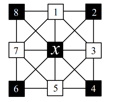
Figure 1 provides an example of two different detection systems on the same 8-vertex graph. In Figure 2 (a) we see that \(L_S(v_1) = \{v_2,v_4,v_5\} \neq \varnothing\) (and similarly for all other vertices) and \(L_S(v_6) = \{v_2,v_5\} \neq \{v_4,v_5\} = L_S(v_8)\) (and similarly for all other distinct pairs), so the shaded vertices in (a) satisfy Theorem 2.7 using \(R_{det}(v) = N(v)\), implying we have an OLD set. Similarly, in Figure 1 (b), we see that \(L_S(v_1) = \{v_1,v_2\} \neq \varnothing\) (and similarly for all other vertices) and \(L_S(v_6) = \{v_2\} \neq \{v_8\} = L_S(v_8)\) (and similarly for all other distinct pairs), so the shaded vertices in (b) satisfy Theorem 2.7 using \(R_{det}(v) = N[v]\), implying we have an IC.
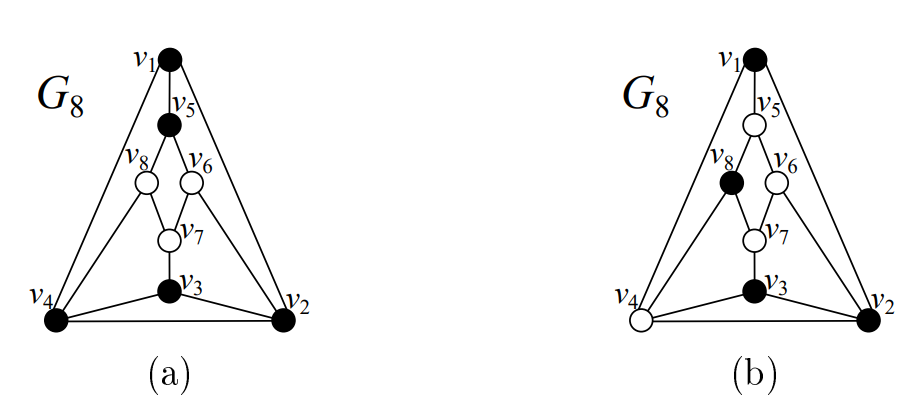
For finite graphs, we use the notations \(\textrm{OLD}(G)\) and \(\textrm{IC}(G)\) (and similarly for any other types of detection systems we will discuss) to denote the cardinality of the smallest possible such sets on graph \(G\), respectively. Since we determined that the OLD and IC sets in Figure 1 were optimal, we find that \(\textrm{OLD}(G_8) = 5\) and \(\textrm{IC}(G_8) = 4\).
For infinite graphs, we cannot meaningfully measure the cardinality of the detection system; rather, we measure the density of the subset, which is defined as \(\limsup_{r \to \infty} \frac{|B_r(v) \cap S|}{|B_r(v)|}\) where \(B_r(v) = \{u \in V(G) : d(u,v) \le r\}\) is the ball of radius \(r\) about \(v\). Importantly, it is possible for the density to vary with the choice of center point \(v\). However, it has been proven that any graph with the “slow-growth” property of \(\lim_{r \to \infty} \frac{|B_{r+1}(v)|}{|B_r(v)|} = 1\) has the additional property that density is invariant of the choice of center point [15]. In this paper, we will only consider graphs which exhibit the slow-growth property; notably, this includes all finite graphs. We use the notations \(\textrm{OLD}\%(G)\) and \(\textrm{IC}\%(G)\) (and similarly for any other types of detection systems we will discuss) to denote the lowest density of any possible such set on \(G\) [11, 16, 20]. Note that density is also defined for finite graphs. If we would prefer to use densities for the sets in Figure 1, we find that \(\textrm{OLD}\%(G_8) = \frac{5}{8}\) and \(\textrm{IC}\%(G_8) = \frac{4}{8}=\frac{1}{2}\).
In the next section, we discuss fault-tolerant variants of detection systems known as \(k\)-redundant detection systems. In Section 3 we explore upper and lower bounds for optimal 1-redundant detection systems on the infinite king grid.
The detection systems we have described in Section 1 are guaranteed to work in all scenarios with at most one intruder under the assumption that there are no faulty sensors. However, depending on the problem, we might require the detection system to be fully functional even when some of the detectors go offline or are broken. For this purpose, we could instead use a fault-tolerant variant of a detection system known as a \(k\)-redundant detection system, which is a detection system for which removing at most \(k\) detectors is still a detection system.
Definition 2.1. A \(k\)-redundant detection system is a detection system \(S \subseteq V(G)\) such that for any \(D \subseteq S\) with \(|D| \le k\), \(S-D\) is a detection system.
By Definition 2.1, a detection system is technically a 0-redundant detection system. In this paper, we will explore redundant open-locating-dominating (RED:OLD) sets and redundant identifying codes (RED:ICs), which are 1-redundant detection systems. These parameters have been explored by several other papers; for instance, RED:OLD sets were first defined and explored in infinite grids [20], and were later explored in arbitrary cubic graphs [17]. Both of these parameters when expressed as decision-based optimization problems have been shown to be NP-Complete [7, 12].
Definition 2.2. A redundant identifying code (RED:IC) is a 1-redundant detection system using \(R_{det}(v) = N[v]\).
Definition 2.3. A redundant open-locating-dominating set (RED:OLD) is a 1-redundant detection system using \(R_{det}(v) = N(v)\).
Next, we present characterizations that will be useful in constructing detection systems.
Definition 2.4. A vertex \(v \in V(G)\) is said to be k-dominated by a set \(S \subseteq V(G)\) if it is dominated (covered) by the detection regions of exactly \(k\) vertices in \(S\). That is, \(|L_S(v)| = k\).
Definition 2.5. [11] A set \(S \subseteq V(G)\) is said to be k-distinguishing if for any two distinct vertices \(u,v \in V(G)\), \(|L_S(u) \triangle L_S(v)| \ge k\).
In this paper, when quantifiers such as “at least” are used with \(k\)-dominated, they apply to the value of \(k\). For instance, “at least 1-dominated” means \(k\)-dominated for some \(k \ge 1\). When the type of detection system is understood, the term “distinguished” denotes \(k\)-distinguished for some \(k\) satisfying the requirements of said detection system. For example, when discussing a RED:OLD set, \(u\) and \(v\) are “distinguished” when they are \(2\)-distinguished.
Definition 2.6. Let \(S \subseteq V(G)\) be a set of detectors. The domination count of a vertex \(v \in V(G)\), denoted \(dom_S(v)\), is \(k\) such that \(v\) is \(k\)-dominated by \(S\).
The notation \(dom_S(v)\) introduced by Definition 2.6 is technically equivalent to \(|L_S(v)|\) but is used in this paper for semantic clarity when only the count is needed.
Theorem 2.7. A set \(S \subseteq V(G)\) is a detection system if and only if all vertices are at least 1-dominated and all pairs are 1-distinguished.
Proof. Consider the properties given in Definition 1.4 and apply the following equivalences: \[\begin{aligned} L_S(v) \neq& \varnothing \Longleftrightarrow |L_S(v)| \ge 1\\ L_S(v) \neq& L_S(u) \Longleftrightarrow L_S(v) \triangle L_S(u) \neq \varnothing \Longleftrightarrow |L_S(v) \triangle L_S(u)| \ge 1. \end{aligned}\] ◻
Theorem 2.8. [20] A set \(S \subseteq V(G)\) is a \(k\)-redundant detection system (\(k \ge 0\)) if and only if all vertices are at least \((k+1)\)-dominated and all pairs are \((k+1)\)-distinguished.
Proof. Let \(S \subseteq V(G)\) be a \(k\)-redundant detection system and \(v \in V(G)\). Suppose \(|L_S(v)| \le k\). Consider the new set \(S' = S-L_S(v)\). Then \(L_{S'}(v) = \varnothing\), implying \(S'\) is not a detection system, a contradiction. Thus, \(|L_S(v)| \ge k + 1\) and we have that \(S\) at least \((k+1)\)-dominates all vertices. Let \(u \in V(G)\) with \(u \neq v\) and let \(D = L_S(u) \triangle L_S(v)\). Suppose that \(|D| \le k\). Consider the new set \(S' = S-D\). We see that \(L_{S'}(u) \triangle L_{S'}(v) = \varnothing\), so \(S'\) is not a detection system, a contradiction. Thus, \(|D| \ge k + 1\) and we have that \(S\) is \((k+1)\)-distinguishing.
For the converse, suppose \(S \subseteq V(G)\) is \((k+1)\)-distinguishing and it at least \((k+1)\)-dominates all vertices. These properties satisfy the requirements of Theorem 2.7, so we know that \(S\) is a detection system. By hypothesis, \(S\) is \((k+1)\)-distinguishing, so \(\forall u,v \in V(G)\) with \(u \neq v\), \(|L_S(u) \triangle L_S(v)| \ge k + 1\). Additionally, \(S\) is at least \((k+1)\)-dominating, so \(\forall v \in V(G),\; |L_S(v)| \ge k + 1\). Let \(D\) be an arbitrary subset of \(S\) with \(|D| \le k\). Consider the new set \(S' = S-D\). The removal of \(|D|\) elements from \(S\) will remove at most \(|D|\) elements from any locating code; thus, \(\forall v \in V(G),\; |L_{S'}(v)| \ge 1\), implying \(S'\) at least 1-dominates all vertices. Additionally, the removal of \(|D|\) elements from \(S\) will remove at most \(|D|\) differences in any pair of locating codes, thus \(\forall u,v \in V(G)\) with \(u \neq v\), \(|L_{S'}(u) \triangle L_{S'}(v)| \ge 1\), so \(S'\) is 1-distinguishing. Therefore, by Theorem 2.7, \(S'\) is a detection system, implying that \(S\) is a \(k\)-redundant detection system. ◻
Note that Theorem 2.8 has been introduced and proven for the specific case where \(k=1\) [20], but we have provided a generalized form here.
Theorem 2.9. Suppose \(S \subseteq V(G)\) at least \(p\)-dominates all vertices and is \(q\)-distinguishing. Then any superset \(S' \supseteq S\) also at least \(p\)-dominates all vertices and is \(q\)-distinguishing.
Proof. Let \(T \subseteq V(G)-S\) with \(T \neq \varnothing\). Let \(S' = S \cup T\). Because \(S\) at least \(p\)-dominates all vertices, \(\forall v \in V(G),\; |L_S(v)| \ge p\). By Definition 1.1, \(L_S(v) = \{x \in S : v \in R_{det}(x)\}\). Therefore, the inclusion of vertices \(T\) as new detectors results in \(L_S(v) \subseteq L_{S'}(v)\), so \(|L_{S'}(v)| \ge p\) and we have that \(S'\) at least \(p\)-dominates all vertices. Additionally, because \(S\) is \(q\)-distinguishing, for any two distinct vertices \(u,v \in V(G),\; |L_S(u) \triangle L_S(v)| \ge q\). By the previous finding, we see that \(L_S(u) \triangle L_S(v) \subseteq L_{S'}(u) \triangle L_{S'}(v)\), so \(|L_{S'}(u) \triangle L_{S'}(v)| \ge q\) and we have that \(S'\) is \(q\)-distinguishing. ◻
Corollary 2.10. Any superset of a \(k\)-redundant detection system is a \(k\)-redundant detection system.
Theorem 2.9 gives us an important fact: if there exists a non-trivial detection system or \(k\)-redundant detection system on some graph, then there also exists a larger one. Therefore, what we are interested in is finding the smallest possible set on a given graph.
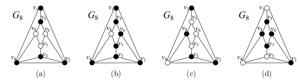
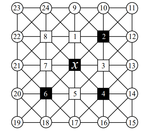
Figure 2 shows examples of a RED:OLD set (b) and a RED:IC (d) on the same same \(G_8\) graph. Images (a) and (c) are copied from Figure 1 for comparison to OLD and IC, respectively. One can verify both (b) and (d) satisfy Theorem 2.8 with \(k=1\) and \(R_{det}(v)\) being \(N(v)\) and \(N[v]\), respectively; so (b) is a RED:OLD set and (d) is a RED:IC. Additionally, one can verify that for any of these sets, no smaller set satisfying the same requirements exists; therefore, these are optimal. Thus, we see that \(\textrm{RED:OLD}(G_8) = 7\) and \(\textrm{RED:IC}(G_8) = 5\).
In this section, we consider RED:OLD sets and RED:ICs on the infinite king grid (\(K\)) an 8-regular graph inspired by chess, with vertices representing positions on an infinite chessboard and edges representing all the normal movements of a king.
Many papers have been published exploring various types of detection systems and other graphical parameters on the king grid. The first such paper—by Cohen, Honkala, and Lobstein [5]—covered the creation of ICs; importantly, they proved that \(\frac{2}{9} \le \textrm{IC}\%(K) \le \frac{4}{17}\). This was soon improved by Charon, Hudry, and Lobstein [4], who demonstrated that \(\textrm{IC}\%(K) = \frac{2}{9}\). Many papers have since been published covering various properties of ICs [3, 6, 8, 9, 14] on finite and infinite king grids. OLD sets in the infinite king grid have been explored by Seo [16] proving \(\frac{6}{25} \le \textrm{OLD}\%(K) \le \frac{1}{4}\). In this section, we will explore upper and lower bounds for \(\textrm{RED:OLD}\%(K)\) and \(\textrm{RED:IC}\%(K)\).
Depending on the graph, directly proving a lower bound for the minimum density of a detection system can be difficult. Instead, it’s often easier to use what’s known as a share argument, established by Slater [21] and used extensively by numerous papers on related concepts of detection systems [11, 16, 18, 19, 20]. For any dominating set (and by extension for any detection system), the inverse of average share is equal to the density. For infinite graphs, we may use the average density within a finite ball and take the limit as the radius approaches infinity; this definition was introduced by Sampaio et al. [15]. Thus, if we find an upper bound for the average share, its inverse is a lower bound for density.
Let \(G\) be a graph, \(S \subseteq V(G)\) be a set of detectors, \(v \in S\), and \(u \in R_{det}(v)\). Vertex \(u\) is dominated exactly \(dom_S(u)\) times, one of which is due to \(v\). Thus, \(v\)’s share in dominating \(u\), denoted \(sh_S[u](v)\), is \(\frac{1}{dom_S(u)}\). And the (total) share of \(v\), denoted \(sh_S(v)\), is \(\sum\limits_{w \in R_{det}(v)}{sh_S[w](v)}\). We will also introduce the following compact notation: where \(A \subseteq R_{det}(v)\), the partial share of \(v\) over \(A\), denoted \(sh_S[A](v)\), is \(\sum\limits_{w \in A}{sh_S[w](v)}\).
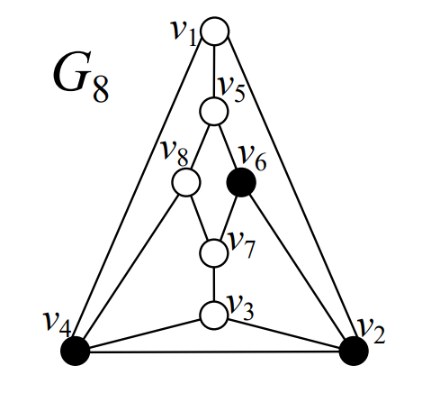
As an example of calculating shares and partial shares, consider the open-dominating set \(S = \{v_2,v_4,v_6\}\) on the \(G_8\) graph in Figure 3. Consider \(v_2 \in S\), which is adjacent to \(\{v_1,v_3,v_4,v_6\}\). \(dom_S(v_4) = dom_S(v_6) = 1\), so \(sh_S[v_4](v_2) = sh_S[v_6](v_2) = \frac{1}{1} = 1\). \(dom_S(v_1) = dom_S(v_3) = 2\), so \(sh_S[v_1](v_2) = sh_S[v_3](v_2) = \frac{1}{2}\). Therefore, \(sh_S(v_2) = sh_S[v_1,v_3,v_4,v_6](v_2) = 1 + 1 + \frac{1}{2} + \frac{1}{2} = 3\). Now consider \(v_4 \in S\), which is adjacent to \(\{v_1,v_2,v_3,v_8\}\). \(dom_S(v_1) = dom_S(v_2) = dom_S(v_3) = 2\) and \(dom_S(v_8) = 1\), so \(sh_S(v_4) = sh_S[v_1,v_2,v_3,v_8](v_4) = \frac{1}{2} + \frac{1}{2} + \frac{1}{2} + 1 = \frac{5}{2}\). And finally, we have \(v_6 \in S\) with \(sh_S(v_6) = \frac{1}{2} + 1 + 1 = \frac{5}{2}\). The average share is \(\frac{1}{3}\left[3 + \frac{5}{2} + \frac{5}{2}\right] = \frac{8}{3}\) and indeed we see that the density of this solution is \(\frac{3}{8}\).
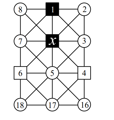
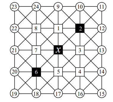
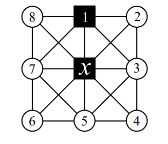
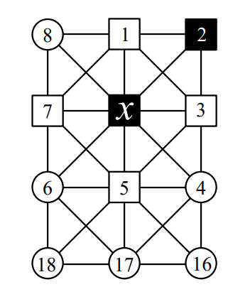
The graphs shown in subsequent figures use circles to represent “unknowns” (vertices which may or may not be detectors), shaded squares to represent detectors, and non-shaded squares to represent non-detectors. Additionally, any vertex labeled simply with number \(k\) will be referred to as \(v_k\) in the text. For instance, in Figure 4, \(\{x,v_1\}\) are detectors, \(\{v_4,v_6\}\) are non-detectors, and everything else is currently unknown.
Let \(S \subseteq V(K)\) be a RED:OLD set on \(K\). Consider the scenario in Figure 4. Vertices \(v_2\), \(v_3\), \(v_7\), and \(v_8\) are dominated by the same two vertices. If one of the four vertices is 2-dominated, then the other three must be at least 4-dominated in order to be distinguished; thus, \(sh_S[v_2,v_3,v_7,v_8](x) \le \frac{1}{2} + \frac{3}{4} = \frac{5}{4}\). Otherwise all four vertices are at least 3-dominated, in which case \(sh_S[v_2,v_3,v_7,v_8](x) \le \frac{4}{3}\). In either case we see that \(sh_S[v_2,v_3,v_7,v_8](x) \le \frac{4}{3}\).
This finding is useful, but it can easily be generalized to any graph and many possible configurations and types of sets:
Lemma 3.1. Suppose \(G\) is a graph, \(S \subseteq V(G)\) is \(k\)-distinguishing with symmetric detection regions \(R_{det}\), \(k \ge 0\), \(D \subseteq S\) is a non-empty set of detectors with \(v \in D\), and \(A \subseteq V(G)\) is a non-empty set of vertices with \(D \subseteq \cap_{u \in A}{R_{det}(u)}\). If \(\exists u \in A\) such that \(dom_S(u) = |D|\), then \(sh_S[A](v) \leq \frac{1}{|D|} + \frac{|A|-1}{|D|+k}\). Otherwise, \(sh_S[A](v) \leq \frac{|A|}{|D|+1}\). In either case, \[sh_S[A](v) \le \begin{cases} \frac{|A|}{|D|+1}, & |A||D|(k-1) \ge (|D|+1)k ,\\ \frac{1}{|D|} + \frac{|A|-1}{|D|+k}, & |A||D|(k-1) < (|D|+1)k. \end{cases}\]
Proof. By hypothesis, \(D \subseteq S\) and \(D \subseteq \cap_{u \in A}{R_{det}(u)}\). Because \(R_{det}\) is symmetric, by Theorem 1.3, \(D \subseteq \cap_{u \in A}{L_S(u)}\). Suppose \(\exists u \in A\) such that \(dom_S(u) = |D|\). Then \(L_S(u) = D\) and we observe that \(\forall w \in A-\{u\},\; |L_S(w) \triangle L_S(u)| = |L_S(w) – D| = |L_S(w)| – |D| = dom_S(w) – |D|\). By hypothesis, \(S\) is \(k\)-distinguishing, so this quantity must be at least \(k\). Therefore, \(dom_S(w)-|D| \ge k\), which of course means \(dom_S(w) \ge |D|+k\). Hence, \(sh_S[A](v) \le \frac{1}{|D|} + \frac{|A|-1}{|D|+k}\). Otherwise \(\forall u \in A,\; dom_S(u) \ge |D|+1\), in which case \(sh_S[A](v) \le \frac{|A|}{|D|+1}\).
In either case \(sh_S[A](v) \le \max\left\{\frac{|A|}{|D|+1}, \frac{1}{|D|} + \frac{|A|-1}{|D|+k}\right\}\). We will now characterize when this is \(\frac{|A|}{|D|+1}\). For convenience, let \(a = |A|\) and \(d = |D|\): \[\begin{aligned} \frac{a}{d+1} &\ge \frac{1}{d} + \frac{a-1}{d+k} \\ ad(d+k) &\ge (d+1)(d+k) + (a-1)(d+1)d \\ ad^2 + adk &\ge d^2 + dk + d + k + ad^2 + ad – d^2 – d \\ adk &\ge dk + k + ad\\ ad(k-1) &\ge (d+1)k. \end{aligned}\] ◻
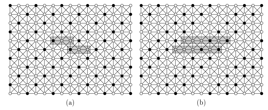
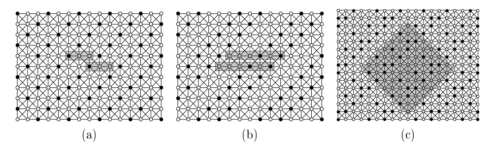
We have found two non-isomorphic RED:OLD sets on the infinite king grid \(K\), as shown in Figure 5. These solutions can be formed via rectangular tilings (regions outlined in the figure). For Figure 5 (a), we see that 1 of the 3 vertices in the tile is a detector (shaded vertices), giving a density of \(\frac{1}{3}\). Similarly, in Figure 5 (b) we see that 2 of the 6 vertices in the tile are used, also giving a density of \(\frac{2}{6} = \frac{1}{3}\). It is also possible to form these solutions by tiling diagonal ribbons of infinite length. For the first solution (a), the ribbon consists of 1 diagonal of detectors and 2 diagonals of non-detectors, giving a density of \(\frac{1}{3}\). For the second solution (b), the ribbon consists of 2 diagonals of detectors and 4 diagonals of non-detectors, giving a density of \(\frac{2}{6} = \frac{1}{3}\). As we have a RED:OLD set on \(K\) with density \(\frac{1}{3}\), we have an upper bound for the optimal density: RED:OLD%(\(K\)) \(\le \frac{1}{3}\).
Let \(S \subseteq V(K)\) be a RED:OLD set on \(K\), and let the notations \(sh\), \(dom\), and \(k\)-dominated implicitly use \(S\). These will persist for the rest of Section .
\(S\) is a 1-redundant detection system, so Theorem 2.8 gives us that every vertex must be at least 2-dominated, so for any detector \(x \in S\) and any neighbor \(v \in N(x)\), \(sh[v](x) \le \frac{1}{2}\). Additionally, \(K\) is an 8-regular graph, so \(|N(x)| = 8\). Therefore, \(sh(x) \le \frac{8}{2} = 4\), giving us a simple lower bound of RED:OLD%(\(K\)) \(\ge \frac{1}{4}\).
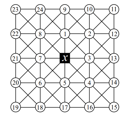
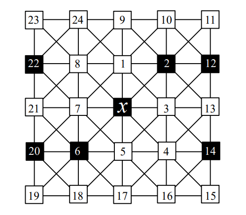
We will now prove another, higher bound. Consider a detector \(x \in S\) and its as-of-yet unknown local region of \(K\), as shown in Figure 6. Suppose that \(\forall w \in N(x),\; dom(w) = 2\). All neighbors of \(x\) are dominated by \(x\) itself. Because the neighbors of \(x\) are all 2-dominated by hypothesis, they must all be dominated exactly one more time. However, if two neighbors of \(x\) are dominated by the same two detectors, then they will not be distinguished. If \(v_9 \in S \lor v_{10} \in S\), then \(\{v_1,v_2\}\) are not distinguished. Likewise, if \(v_1 \in S\), then \(\{v_2,v_3\}\) are not distinguished. And if \(v_2 \in S\), then \(\{v_1,v_3\}\) are not distinguished. By symmetry, the only vertices in the figure which can possibly be detectors are \(\{v_{11},v_{15},v_{19},v_{23}\}\), but this means that \(\forall w \in \{v_1,v_3,v_5,v_7\},\; dom(w) = 1\), contradicting that \(S\) is a RED:OLD set on \(K\). Therefore, \(\exists w \in N(x)\) such that \(dom(w) \ge 3\), so \(sh[w](x) \le \frac{1}{3}\). By Theorem 2.8, any RED:OLD set at least 2-dominates every vertex, thus, where \(u \in N(x)\), \(dom(u) \ge 2\), thus \(sh[u](x) \le \frac{1}{2}\). Thus, \(sh_S(x) \le \frac{7}{2} + \frac{1}{3} = \frac{23}{6}\), meaning we have a higher lower bound: RED:OLD%(\(K\)) \(\ge \frac{6}{23}\).
At this point, we have two lower bounds for RED:OLD%(\(K\)): \(\frac{1}{4}\) and \(\frac{6}{23}\). These are both still relatively far from our upper bound of \(\frac{1}{3}\). To help bridge the gap between upper and lower bounds, we would now like to prove a significantly more ambitious lower bound of \(\frac{3}{10}\), which will require demonstrating an upper bound for average share of \(\frac{10}{3}\).
Theorem 3.2. In any RED:OLD set \(S\) on \(K\), the average share over all vertices in \(S\) is no larger than \(\frac{10}{3}\).
Proof. Let \(x \in S\) be an arbitrary vertex in the RED:OLD set \(S\). We will explore all non-isomorphic configurations and show that the average share it gives rise to is at most \(\frac{10}{3}\).
Case 1. We begin by considering when \(x\) is dominated by two neighbors in a “bent” shape, as in Figure 7. We will demonstrate that in any possible sub-configuration \(sh(x) \le \frac{13}{4} < \frac{10}{3}\).
From the figure we clearly see that \(dom(v_3) \ge 3\). Suppose \(dom(v_3) = 3\). By Lemma 3.1, \(sh[v_2,v_3,v_7,v_8](x) \le \frac{4}{3}\). Additionally, \(dom(v_5) \ge 3\) in order to be distinguished from \(v_3\). Since each of the other three vertices in \(N(x)\) is at least 2-dominated, we have \(sh[v_1,v_4,v_6](x) \le \frac{3}{2}\). Thus, \(sh(x) \le \frac{4}{3} + \frac{1}{3} + \frac{3}{2} = \frac{19}{6} < \frac{13}{4}\). Otherwise \(dom(v_3) \ge 4\). Then, by Lemma 3.1, \(sh[v_2,v_7,v_8](x) \le 1\), and each of the other four vertices in \(N(x)\) is at least 2-dominated, we have \(sh[v_1,v_4,v_5,v_6](x) \le \frac{4}{2}\). Thus, \(sh(x) \le 1 + \frac{1}{4} + \frac{4}{2} = \frac{13}{4}\).
Case 2. Next, we consider when \(x\) is dominated by vertex \(v_1\) directly above it, as in Figure 8. We will demonstrate that in any sub-configuration \(sh(x) \le \frac{13}{4} < \frac{10}{3}\).
From Case 1 we know that if \(\{v_4,v_6\} \cap S \neq \varnothing\), then \(sh(x) \le \frac{13}{4}\) and we are done. Therefore, we assume that neither of these is a detector. Suppose that \(\forall w \in \{v_4,v_5,v_6\},\; dom(w)\\ = 2\). If \(v_{17} \in S\), then \(\{v_4,v_5\}\) are impossible to distinguish due to both being 2-dominated by hypothesis; thus, \(v_{17} \notin S\). By the same logic, \(v_{16} \notin S\) and \(v_3 \notin S\). Likewise, if \(v_{18} \in S\), then \(\{v_5,v_6\}\) are impossible to distinguish. By the same logic, \(v_7 \notin S\). We therefore find that \(dom(v_5) = 1\), contradicting that \(S\) is a RED:OLD set. Therefore, \(\exists w \in \{v_4,v_5,v_6\}\) such that \(dom(w) \ge 3\). Additionally, by Lemma 3.1, \(sh[v_2,v_3,v_7,v_8](x) \le \frac{4}{3}\). Therefore, \(sh(x) \le \frac{4}{3} + \frac{1}{3} + \frac{3}{2} = \frac{19}{6} < \frac{13}{4}\).
Case 3. We now consider when \(x\) is dominated by four neighbors in an “x” shape, as shown in Figure 9. From Cases 1–2 we see that if \(\{v_1,v_3,v_5,v_7\} \cap S \neq \varnothing\), then \(sh(x) \le \frac{13}{4}\) and we are done. Otherwise, we observe that \(\forall w \in \{v_1,v_3,v_5,v_7\},\; dom(w) \ge 3\). Thus \(sh(x) \le \frac{4}{3} + \frac{4}{2} = \frac{10}{3}\).
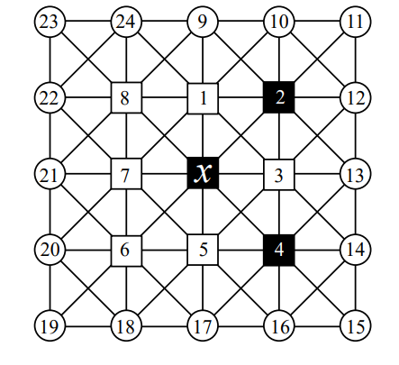
Case 4. We now consider the case where \(x\) is dominated by three neighbors in a “lambda” shape, as in Figure 10. From Cases 1–3 we know that if \(\{v_1,v_3,v_5,v_7,v_8\} \cap S \neq \varnothing\), then \(sh(x) \le \frac{10}{3}\). Therefore we assume \(\{v_1,v_3,v_5,v_7,v_8\} \cap S = \varnothing\) and consider the sub-cases depending the values of \(dom(v_3)\) and \(dom(v_5)\) as follows.
First, suppose \(dom(v_3) = 6\) or \(dom(v_5) = 6\). If \(dom(v_3) = 6\), then \(\{v_{12},v_{13},v_{14}\} \subseteq S\). This makes \(dom(v_2) \ge 3\) and \(dom(v_4) \ge 3\). Additionally, we have that \(dom(v_5) \ge 3\) by hypothesis. Therefore, \(sh(x) \le \frac{1}{6} + \frac{3}{3} + \frac{4}{2} = \frac{19}{6} < \frac{10}{3}\). By symmetry, we get the same results when \(dom(v_5) = 6\).
Next, we consider when \(dom(v_3) = 3\). We observe that \(dom(v_3) = 3\) requires \(dom(v_1) \ge 3\). If we have \(dom(v_5) = 3\), then it also requires \(dom(v_7) \ge 3\), hence we obtain \(sh(x) \le \frac{4}{3} + \frac{4}{2} = \frac{10}{3}\) and we are done. Therefore, we assume that \(dom(v_5) \ge 4\). Currently, we have three vertices, namely \(v_1\), \(v_3\), and \(v_5\), which are at least 3-dominated. If \(\exists w \in \{v_2,v_4,v_6,v_7,v_8\}\) such that \(dom(w) \ge 3\), then \(sh(x) \le \frac{4}{3} + \frac{4}{2} = \frac{10}{3}\) and we are done. Therefore, we assume \(\forall w \in \{v_2,v_4,v_6,v_7,v_8\},\; dom(w) = 2\). By hypothesis, we have \(dom(v_7) = 2\), thus \(\{v_{20},v_{21},v_{22}\} \cap S = \varnothing\). Presently, \(dom(v_8) = 1\) and there are three unknown vertices, \(\{v_9,v_{23},v_{24}\}\) which can possibly second-dominate \(v_8\). If \(v_9 \in S\), then \(\{v_2,v_8\}\) are not distinguished, a contradiction. If \(v_{23} \in S\), then \(v_{24} \notin S\) leaving only \(v_{10}\) to have \(dom(v_1) \ge 3\), but this makes \(\{v_1,v_2\}\) impossible to distinguish, a contradiction. Therefore, the only way to have \(dom(v_8) = 2\) requires \(v_{24} \in S\), and this results in \(dom(v_1) \ge 4\) because \(\{v_1,v_8\}\) would not be distinguished, otherwise. Thus \(sh(x) \le \frac{2}{4} + \frac{1}{3} + \frac{5}{2} = \frac{10}{3}\). By symmetry, if \(dom(v_5) = 3\), we get the same results.
Now, we will proceed with the remaining possibilities for the domination of \(\{v_3,v_5\}\). Due to symmetry, without loss of generality let \(4 \le dom(v_3) \le dom(v_5) \le 5\) and we consider the following three configurations; \(dom(v_3) = 5 = dom(v_5)\), \(dom(v_3) = 4 \le 5 = dom(v_5)\), and \(dom(v_3) = 4 = dom(v_5)\).
If we want to achieve \(dom(v_3) = 5 = dom(v_5)\), any possible way to do this results in \(dom(v_4) \ge 3\). Thus, \(sh(x) \le \frac{2}{5} + \frac{1}{3} + \frac{5}{2} = \frac{97}{30} < \frac{10}{3}\).
Now, we assume that \(dom(v_3) = 4 \le 5 = dom(v_5)\). We initially observe that if there exists some \(w \in \{v_1,v_2,v_4,v_6,v_7,v_8\}\) such that \(dom(w) \ge 3\), then \(sh(x) \le \frac{1}{5} + \frac{1}{4} + \frac{1}{3} + \frac{5}{2} = \frac{197}{60} < \frac{10}{3}\). Thus, we need only consider when \(\forall w \in \{v_1,v_2,v_4,v_6,v_7,v_8\},\; dom(w) = 2\). Suppose \(v_{17} \in S\), then \(dom(v_4) \ge 3 \lor dom(v_6) \ge 3\) in order to be distinguished, a contradiction. By hypothesis, \(dom(v_5) = 5\), so \(v_{17} \notin S \land \{v_{16},v_{18}\} \subseteq S\). Because \(dom(v_1) = 2\), \(\{v_9,v_{10},v_{24}\} \cap S = \varnothing\). Similarly, \(dom(v_7) = 2\), requiring \(\{v_{20},v_{21},v_{22}\} \cap S = \varnothing\). Then \(v_{23} \in S\) to make \(dom(v_8) \ge 2\), and \(v_{19} \notin S\) because \(dom(v_6) = 2\). We also see that \(dom(v_4) = 2\), which means \(\{v_{13},v_{14},v_{15}\} \cap S = \varnothing\). This means \(v_{12} \in S\) because \(dom(v_3) = 4\), and \(v_{11} \notin S\) because \(dom(v_2) = 2\). This leads to the sub-configuration shown in Figure 11 (a). We see that \(sh(x) = \frac{1}{5} + \frac{1}{4} + \frac{6}{2} = \frac{69}{20} > \frac{10}{3}\). However, we observe that \(x\) is adjacent to \(\{v_2,v_4,v_6\} \subseteq S\), all of which have “bent” shape; thus, as demonstrated in Case 1, \(\forall w \in \{v_2,v_4,v_6\},\; sh(w) \le \frac{13}{4} < \frac{10}{3}\). Additionally, the only other detectors these 3 vertices are adjacent to are \(\{v_{12},v_{16},v_{18}\}\), all of which are adjacent via vertical or horizontal edges. Thus, the findings of Cases 1 and 2 tell us that \(\forall w \in \{v_{12},v_{16},v_{18}\},\; sh(w) \le \frac{13}{4} < \frac{10}{3}\). Therefore, we are safe to use \(\{x,v_2,v_4,v_6\}\) in an averaging argument; consider the average share: \(\frac{1}{4} \left[ \frac{69}{20} + \frac{13}{4} + \frac{13}{4} + \frac{13}{4} \right] = \frac{33}{10} < \frac{10}{3}\). Hence, we have that the average share is still no larger than \(\frac{10}{3}\).
As the last sub-case, we have \(dom(v_3) = 4 = dom(v_5)\). We initially observe that if \(\exists w \in \{v_1,v_2,v_4,v_6,v_7,v_8\}\) such that \(dom(w) \ge 3\), then \(sh(x) \le \frac{2}{4} + \frac{1}{3} + \frac{5}{2} = \frac{10}{3}\). Thus, we need only consider when \(\forall w \in \{v_1,v_2,v_4,v_6,v_7,v_8\},\; dom(w) = 2\). Because \(dom(v_4) = 2\), at most one of the additional detectors for \(v_3\) and \(v_5\) can be in \(N(v_4)\). Due to symmetry, without loss of generality let the additional detector for \(v_3\) not be in \(N(v_4)\); \(\{v_{13},v_{14}\} \subseteq N(v_4)\), so \(v_{12} \in S \land v_{13} \notin S \land v_{14} \notin S\). Additionally, because \(dom(v_2) = 2\) by hypothesis, \(v_{11} \notin S\). We also see that \(dom(v_1) = dom(v_7) = 2\), implying \(\{v_9,v_{10},v_{20},v_{21},v_{22},v_{24}\} \cap S = \varnothing\). This requires \(v_{23} \in S\) to make \(dom(v_8) \ge 2\). If \(v_{17} \in S\), then \(\{v_4,v_6\}\) are impossible to distinguish; thus, \(v_{17} \notin S\). By hypothesis, \(dom(v_6) = 2\); thus exactly one of \(\{v_{18},v_{19}\}\) must be a detector. We will now consider two cases: \(v_{19} \in S\) or \(v_{19} \notin S\).
If \(v_{19} \in S\), then \(v_{18} \notin S\). By hypothesis, \(dom(v_5) = 5\), so \(v_{16} \in S\), and by hypothesis \(dom(v_4) = 2\), requiring \(v_{15} \notin S\). This leads to the sub-configuration shown in Figure 11 (b). \(sh(x) = \frac{2}{4} + \frac{6}{2} = \frac{7}{2} > \frac{10}{3}\). However, as demonstrated previously in this case we can safely average with the adjacent “bent” shape vertices \(\{v_2,v_4\}\), which have share no more than \(\frac{13}{4} < \frac{10}{3}\). \(\frac{1}{3} \left[ \frac{7}{2} + \frac{13}{4} + \frac{13}{4} \right] = \frac{10}{3}\). Thus in this terminal sub-configuration, we still have that the average share is no more than \(\frac{10}{3}\).
If \(v_{19} \notin S\), then \(v_{18} \in S\). Then, by similar logic to the previous paragraph, \(v_{16} \notin S \land v_{15} \in S\). We now have the sub-configuration shown in Figure 11 (c). This again has \(sh(x) = \frac{2}{4} + \frac{6}{2} = \frac{7}{2} > \frac{10}{3}\). However, we also still have 2 “bent” shape neighbors of \(x\): \(\{v_2,v_6\}\), which are safe to use for averaging by the same logic, as demonstrated previously in this case. Thus, we once again have the average share \(\frac{1}{3} \left[ \frac{7}{2} + \frac{13}{4} + \frac{13}{4} \right] = \frac{10}{3}\).
Case 5. We now consider when \(x\) is dominated by two neighbors in a diagonal, as in Figure 12. By applying the results of Cases 1–4 we see that if \(\{v_1,v_3,v_4,v_5,v_7,v_8\} \cap S \neq \varnothing\), then the average share is no larger than \(\frac{10}{3}\) and we are done. Thus we need only consider when \(\{v_1,v_3,v_4,v_5,v_7,v_8\} \cap S = \varnothing\). We observe that \(dom(v_1) \le 5\). Suppose that \(dom(v_1) = 5\), then \(dom(v_2) \ge 3 \land dom(v_8) \ge 3\). Additionally, \(\{v_5,v_7\}\) are not distinguished, so at least one of them must be at least 3-dominated. Thus \(sh(x) \le \frac{1}{5} + \frac{3}{3} + \frac{4}{2} = \frac{16}{5} < \frac{10}{3}\). By symmetry if \(\exists w \in \{v_1,v_3,v_5,v_7\}\) such that \(dom(w) \ge 5\), then \(sh(x) \le \frac{10}{3}\). Therefore, we need only consider when \(\forall w \in \{v_1, v_3, v_5, v_7\},\; 2 \le dom(w) \le 4\). We will break these into sub-cases by considering the vertex pair \((v_1, v_3)\). Due to symmetry, without loss of generality, let \(dom(v_1) \le dom(v_3)\).
If \(dom(v_1) = 4 = dom(v_3)\), then \(dom(v_2) \ge 3\). Thus, \(sh(x) \le \frac{2}{4} + \frac{1}{3} + \frac{5}{2} = \frac{10}{3}\).
Now consider when \(dom(v_1) = 3 \le 4 = dom(v_3)\). \(\{v_5,v_7\}\) are not yet distinguished, so at least one of them is at least 3-dominated. If the additional third detector for \(v_1\) is \(v_9\) or \(v_{10}\), then \(dom(v_2) = 3\); thus, \(sh(x) \le \frac{3}{3} + \frac{1}{4} + \frac{4}{2} = \frac{13}{4} < \frac{10}{3}\). So we need only consider when the additional third detector for \(v_1\) is \(v_{24} \in S\). We then observe that \(\{v_1,v_8\}\) are not distinguished, requiring \(dom(v_8) \ge 3\). Thus \(sh(x) \le \frac{3}{3} + \frac{1}{4} + \frac{4}{2} = \frac{13}{4} < \frac{10}{3}\).
Next consider when \(dom(v_1) = 3 = dom(v_3)\). Again note that \(\{v_5,v_7\}\) are not distinguished, so at least one of them must be at least 3-dominated. We currently have three neighbors of \(x\) which are at least 3-dominated; if we find one more, then \(sh(x) \le \frac{4}{3} + \frac{4}{2} = \frac{10}{3}\). If both of the additional detectors around \(v_1\) and \(v_3\) are in \(N(v_2)\), then \(dom(v_2) \ge 3\) and we are done. So we assume at least one of the additional detectors is not in \(N(v_2)\); due to symmetry, without loss of generality let \(v_{24} \in S\). Because \(dom(v_3) = 3\) by hypothesis, \(|\{v_{12},v_{13},v_{14}\} \cap S| = 1\). If \(v_{12} \in S \lor v_{13} \in S\), then \(\{v_2,v_3\}\) are not distinguished, requiring \(dom(v_2) = 3\), and we are done. Similarly, if \(v_{14} \in S\), then \(\{v_3,v_4\}\) are not distinguished, requiring \(dom(v_4) \ge 3\), and we are done. In any case we see that \(sh(x) \le \frac{10}{3}\).
If \(dom(v_1) = 2 \land dom(v_3) < 4\), then \(\{v_1, v_3\}\) are impossible to distinguish and thus the configuration is invalid. Otherwise we have the final possibility: \(dom(v_1) = 2 \le 4 = dom(v_3)\). Again note that \(\{v_5,v_7\}\) are not distinguished, so at least one of them must be at least 3-dominated. Because \(dom(v_1) = 2\), \(\{v_9,v_{10},v_{24}\} \cap S = \varnothing\). We now consider the 2 additional detectors in \(N(v_3)\). If \(\{v_{12},v_{13}\} \subseteq S\), then \(v_{14} \notin S\). We observe that \(\{v_2,v_3\}\) are not distinguished, requiring \(v_{11} \in S\), making \(dom(v_2) = 4\). Thus, \(sh(x) \le \frac{2}{4} + \frac{1}{3} + \frac{5}{2} = \frac{10}{3}\). Otherwise if \(\{v_{13},v_{14}\} \subseteq S\), then \(v_{12} \notin S\). If \(v_{11} \in S\), then we have at least 4 vertices which are at least 3-dominated and so \(sh(x) \le \frac{4}{3} + \frac{4}{2} = \frac{10}{3}\); so we consider only when \(v_{11} \notin S\). We see that \(\{v_2,v_4\}\) are not distinguished, requiring \(dom(v_4) \ge 4\). Thus, \(sh(x) \le \frac{2}{4} + \frac{1}{3} + \frac{5}{2} = \frac{10}{3}\). Otherwise we have the final possible sub-configuration: \(\{v_{12},v_{14}\} \subseteq S\), which means \(v_{13} \notin S\). We now look to vertex pair \((v_5,v_7)\), which is symmetric to the the pair \((v_1,v_3)\) we have thus far been using. We applying the same arguments to \((v_5,v_7)\): consider \(A = \{v_{16},v_{17},v_{18},v_{20},v_{21},v_{22}\} \cap S\). By symmetry, any value of \(A\) other than \(\{v_{16},v_{18}\}\) or \(\{v_{20},v_{22}\}\) results in \(sh(x) \le \frac{10}{3}\). If \(A = \{v_{16},v_{18}\}\), then \(dom(v_4) \ge 3\) and we are done, so we assume \(A = \{v_{20},v_{22}\}\). Thus, \(dom(v_3) = dom(v_7) = 4\). We see that if \(\{v_{11},v_{15},v_{19},v_{23}\} \cap S \neq \varnothing\), then we have an additional neighbor of \(x\) which is at least 3-dominated, so \(sh(x) \le \frac{2}{4} + \frac{1}{3} + \frac{5}{2} = \frac{10}{3}\). So we consider only the event when \(\{v_{11},v_{15},v_{19},v_{23}\} \cap S = \varnothing\) and arrive at the sub-configuration in Figure 13.
Figure 13 represents the final possible sub-configuration for Case 5, and we find that \(sh(x) = \frac{7}{2} > \frac{10}{3}\). We observe that \(x\) has two neighbors, \(\{v_2,v_6\}\), of “bent” shape, which in Case 1 was found to have share no more than \(\frac{13}{4}\). Additionally, these two vertices are only adjacent to two other detector vertices \(\{v_{12},v_{20}\} \subseteq S\), and are connected via a horizontal edge, which Cases 1–2 have proven to have share no more than \(\frac{13}{4}\). Thus \(\{v_2,v_6\}\) are not adjacent to any other vertices with share exceeding \(\frac{10}{3}\) and so are safe to use with averaging. Consider the average share of \(\{x,v_2,v_6\}\): \(\textrm{avg} \le \frac{1}{3} \left[ \frac{7}{2} + \frac{13}{4} + \frac{13}{4} \right] = \frac{10}{3}\).
Case 6. In the final case, we consider when \(x\) is dominated by two neighbors in a “wedge” shape like Figure 14. Applying the cumulative results of Cases 1–5 we see that if \(\{v_1,v_3,v_5,v_6,v_7,v_8\} \cap S \neq \varnothing\), then the average share is no more than \(\frac{10}{3}\). We will proceed by expanding every possible state for the neighborhood of \(v_7\). Vertex \(v_7\) must be at least 2-dominated, so we consider all sub-cases for \(2 \leq dom(v_7) \le 4\).
First, we consider when \(dom(v_7) = 4\), which requires \(\{v_{20},v_{21},v_{22}\} \subseteq S\). This implies that \(\forall w \in \{v_6,v_7,v_8\},\; dom(w) \ge 3\). Additionally, \(dom(v_3) \ge 3\) by hypothesis. Thus, \(sh(x) \le \frac{4}{3} + \frac{4}{2} = \frac{10}{3}\).
There are two non-isomorphic ways to have \(dom(v_7) = 3\): one with \(\{v_{21}, v_{22}\} \subseteq S\) and the other with \(\{v_{20}, v_{22}\} \subseteq S\). In either way, \(\{v_6,v_7\}\) are not distinguished, nor are \(\{v_7,v_8\}\). This requires \(dom(v_6) \ge 3\) and \(dom(v_8) \ge 3\). Then \(\forall w \in \{v_3,v_6,v_7,v_8\},\; dom(w) \ge 3\). Thus, \(sh(x) \le \frac{4}{3} + \frac{4}{2} = \frac{10}{3}\).
Finally, there are two non-isomorphic ways to have \(dom(v_7) = 2\): one with \(v_{22} \in S\) and the other with \(v_{21} \in S\). If we have \(dom(v_7) = 2\) with \(v_{22} \in S\), we find that \(\{v_7,v_8\}\) are not distinguished, requiring \(dom(v_8) \ge 4\), which in turn requires \(dom(v_1) \ge 3\). Currently, we have three neighbors of \(x\) which are at least 3-dominated; if we can find a fourth, then \(sh(x) \le \frac{4}{3} + \frac{4}{2} = \frac{10}{3}\) and we will be done. Thus, if \(\exists w \in \{v_4, v_5, v_6\}\) such that \(dom(w) \ge 3\), then we are done, so we assume \(\forall w \in \{v_4, v_5, v_6\},\; dom(w) = 2\). Vertex \(v_5\) is already dominated by 2 neighbors, so \(\{v_{16},v_{17},v_{18}\} \cap S = \varnothing\). We see that \(\{v_3,v_5\}\) are not distinguished, requiring \(dom(v_3) \ge 4\). Therefore we have that \(dom(v_8) \ge 4\), \(dom(v_3) \ge 4\), and \(dom(v_1) \ge 3\), so \(sh(x) \le \frac{2}{4} + \frac{1}{3} + \frac{5}{2} = \frac{10}{3}\). If we have \(dom(v_7) = 2\) with \(v_{21} \in S\), then we observe that \(\{v_6,v_7\}\) are not distinguished, nor are \(\{v_7,v_8\}\). This requires \(dom(v_6) \ge 4\) and \(dom(v_8) \ge 4\), which in turn makes \(dom(v_1) \ge 3\) and \(dom(v_5) \ge 3\). As we already have that \(dom(v_3) \ge 3\), \(sh(x) \le \frac{2}{4} + \frac{3}{3} + \frac{3}{2} = 3 < \frac{10}{3}\). ◻
From Theorem 3.2, we have that the average share for any RED:OLD set on \(K\) is no more than \(\frac{10}{3}\). Thus, \(\frac{3}{10}\) is a lower bound for RED:OLD%(\(K\)).
Corollary 3.3. \(\textrm{RED:OLD}\%(K) \ge \frac{3}{10}.\)
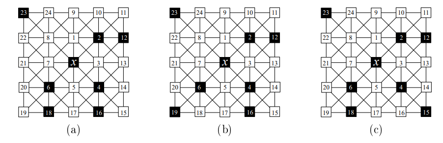
We have found three RED:ICs on \(K\), with density \(\frac{1}{3}\), as shown in Figure 15. Solutions (a) and (b) are identical to the RED:OLD solutions in Figure 5—that is, these two solutions are both RED:OLD and RED:IC. However, Figure 15 (c) is not a RED:OLD set due to some of the vertices being only 1-dominated if open neighborhoods were used. One can easily verify that all of these solutions are RED:ICs via Theorem 2.8 with \(k=1\) and \(R_{det}(v) = N[v]\). Therefore, we have an upper bound for the optimal density: RED:IC%(\(K\)) \(\le \frac{1}{3}\).
Let \(S \subseteq V(G)\) be a RED:IC on \(K\), and let the notations \(sh\), \(dom\), and \(k\)-dominated implicitly use \(S\). These will persist for the rest of Section .
\(S\) is a 1-redundant detection system, so Theorem 2.8 gives us that every vertex is at least 2-dominated. Additionally, \(K\) is 8-regular, so \(|N[v]| = 9\). Therefore, \(\forall x \in S,\; sh(x) \le \frac{9}{2}\). Thus, we have a simple lower bound: RED:IC%(\(K\)) \(\ge \frac{2}{9}\).
Theorem 3.4. The share of any given detector in \(S\) is at most \(\frac{11}{3}\).
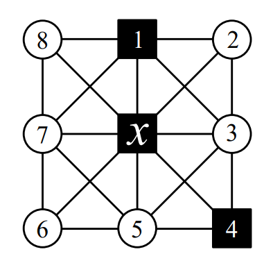
Proof. Just as in the previous section for proving a lower bound for RED:OLD%(\(K\)), we consider a detector \(x \in S\) and its local region of \(K\). Vertex \(x\) must be at least 2-dominated and dominates itself, so we consider the following two cases for the other detector being horizontal/vertical to \(x\) or being diagonal to \(x\), and show \(sh(x) \le \frac{11}{3}\).
Case 1. First, we consider when \(v_1 \in S\) and everything else is unknown, as in Figure 16. Consider \(D = \{x,v_1\}\) and \(A = \{x,v_1,v_2,v_3,v_7,v_8\}\). By Lemma 3.1, \(sh[A](x) \le \frac{6}{2+1} = 2\). We can assume the other three vertices \(\{v_4,v_5,v_6\}\) are at least 2-dominated. Therefore, \(sh(x) \le 2 + \frac{3}{2} = \frac{7}{2} < \frac{11}{3}\).
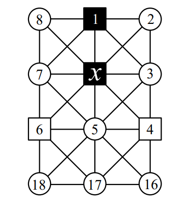
Case 2. Now we consider the only other case, when \(v_2 \in S\). From the results of Case 1, we know that if \(\{v_1,v_3,v_5,v_7\} \cap S \neq \varnothing\), then \(sh(x) \le \frac{11}{3}\); so we assume \(\{v_1,v_3,v_5,v_7\} \cap S = \varnothing\), as shown in Figure 17. Let \(D = \{x,v_2\}\) and \(A = \{x,v_1,v_2,v_3\}\); by Lemma 3.1, \(sh[A](x) \le \frac{4}{2+1} = \frac{4}{3}\). Suppose \(\forall w \in \{v_4,v_5,v_6\},\; dom(w) = 2\).
We will focus on \(v_5\), which by hypothesis is 2-dominated, so there must be a detector in \(N[v_5]\) other than \(x\). However, if the second detector is in \(N[v_4] \cap N[v_5]\), then \(\{v_4,v_5\}\) will share them both and therefore not be distinguished; thus, \(\{v_4,v_{16},v_{17}\} \cap S = \varnothing\). Similarly, if the second detector is in \(N[v_5] \cap N[v_6]\), then \(\{v_5,v_6\}\) will not be distinguished; thus, \(\{v_6,v_{17},v_{18}\} \cap S = \varnothing\). Thus, we have \(\{v_4,v_6,v_{16},v_{17},v_{18}\} \cap S = \varnothing\), which results in \(dom(v_5) =1\), a contradiction. Therefore, \(\exists w \in \{v_4,v_5,v_6\}\) such that \(dom(w) \ge 3\), making \(sh(x) \le \frac{4}{3} + \frac{1}{3} + \frac{4}{2} = \frac{11}{3}\) and we are done. ◻
From Theorem 3.4, we have that the average share for any RED:IC on \(K\) is no more than \(\frac{11}{3}\). Thus, \(\frac{3}{11}\) is a lower bound for RED:IC%(\(K\)).
Corollary 3.5. \(\textrm{RED:IC%}(K) \ge \frac{3}{11}\).
We have now demonstrated that \(\frac{3}{10} \le \textrm{RED:OLD}\%(K) \le \frac{1}{3}\) and \(\frac{3}{11} \le \textrm{RED:IC}\%(K) \le \frac{1}{3}\). Interestingly, both of the RED:OLD sets achieving the upper bound of \(\frac{1}{3}\) (see Figure 5) were also RED:ICs (see Figure 15); however, Figure 15 (c) is not a RED:OLD set.