
A plane graph \(G\) is a graph drawn in the plane (or on the sphere) in which no two edges cross. In this paper, we explore one of the most famous theorems in all of graph theory relating to plane graphs: the Four Color Theorem. One statement of the Four Color Theorem is given below.
Theorem 1.1. The regions of a plane graph \(G\) can be colored with at most 4 colors such that no two adjacent regions (that is, regions sharing a boundary line) have the same color.
Such a coloring is known as a (proper) coloring of the regions of \(G\). The Four Color Theorem has a rich and fascinating history. In 1879, Alfred Bray Kempe famously (or perhaps infamously) attempted to prove the Four Color Theorem using what are now called “Kempe chains.” Given a partially colored plane graph \(G\) and two colors \(A, B\), we can define an \(AB\) Kempe chain as a maximal set of connected regions of \(G\) containing only colors \(A\) and \(B\). A color exchange on an \(AB\) Kempe chain is the result of permuting the colors \(A\) and \(B\) on the Kempe chain. Kempe believed that a simple sequence of color exchanges on these connected components would always be able to produce a four coloring of a plane graph from a partial coloring of all regions excepting one region having at most 5 neighbors (see [6, 10]). This approach was ultimately disproven by Heawood in [4]. While there are computer-assisted proofs of the Four Color Theorem, notably those in [1] and later in [9], these are “machine-checkable proofs” and have not been checked by human readers.
While Kempe’s own attempt was flawed, the idea of Kempe color exchanges on Kempe chains is much easier to grasp than the computational approaches in [1] and [9], and it has proven very effective in practice. It has been demonstrated in [3, 5, 8] that randomly applying color exchanges to Kempe chains has a very high success rate in being able to color a plane graph in relatively few exchanges (see Section 6 for a more precise description of how these exchanges are used). The question, however, is still open if this method will ever get “stuck,” or if using sequences of Kempe chain exchanges will always resolve any issues in coloring. Notably, proof of such a fact would be a proof of the Four Color Theorem, so we anticipate such a proof to be quite challenging.
Instead of applying random color exchanges, we can explore systematic applications of specific color exchanges. This was studied by Alfred Errera in 1921 [2], and more recently by Weiguo Xie in [11, 12, 13]. In both cases the authors consider coloring the regions of cubic maps, where a cubic map is a \(2\)-connected \(3\)-regular plane graph. It is known that showing that the regions of all cubic maps can be properly four-colored is equivalent to proving the Four Color Theorem.
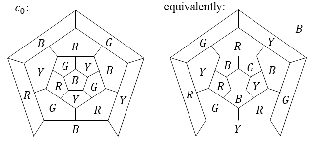
In [2], Errera produced a map with a rather unusual property: given a partial coloring of the map so that all but one region (in this case, all but the exterior region) are colored, and given a particular method of routinely applying Kempe color exchanges, the graph returns to its original coloring after \(20\) such exchanges. Therefore, this coloring fails to reach a state where the exterior region can be colored using this method. As Errera was hoping to prove the Four Color Theorem using this technique, the existence of this counterexample was troublesome. Errera’s map is shown in Figure 1, as presented in [7]. For future reference, we will denote this partial coloring of the Errera map \(c_0\).
In this paper, we will thoroughly examine Errera’s counterexample, determine how to resolve the partial coloring into a proper four-coloring of the entire map, and see how this method can be expanded to a larger class of graphs.
In 1935, Errera’s work was expanded by Irving Kittell, who defined eight different ways to perform Kempe color exchanges on the regions of a map (see [7]). The “random color exchanges” mentioned previously are typically applications of Kittell’s operations. Of those operations, several will be of interest to us. We will assume in the following definitions that the exterior region is the uncolored region, that the exterior region has five neighboring regions, and that these neighboring regions contain all four colors. (Later, we will modify these assumptions to account for graphs with more than one uncolored region, but they are sufficient for the time being.) This means that one color is used twice amongst the neighboring regions. For brevity, we will call the colored regions adjacent to the uncolored region boundary regions. The following notation and definitions are taken from [7], with some rephrasing and adaptation. We will refer to the coloring in Figure 1 for examples.
\(\bullet\) The boundary region situated between two boundary regions of the same color is called the vertex. In Figure 1, this is the boundary region labeled \(R\).
\(\bullet\) A Kempe chain containing both the vertex and the boundary region positioned two spaces clockwise from the vertex is called the left-hand circuit. We may also refer to this circuit by its colors; in Figure 1, we would call the left-hand circuit the \(RG\) circuit. If such a Kempe chain does not exist, we will refer to the Kempe chain using these colors and starting at the vertex as a broken left-hand circuit.
\(\bullet\) Similarly, a Kempe chain containing both the vertex and the boundary region positioned two spaces counterclockwise from the vertex is called the right-hand circuit. In Figure 1, we would call this the \(RY\) circuit. We analogously define broken right-hand circuit.
\(\bullet\) A Kempe chain beginning at the boundary region clockwise to the vertex and whose other color is that of the region two spaces counterclockwise of the vertex (in Figure 1, \(B\) and \(Y\)) is called the left-hand chain.
\(\bullet\) A Kempe chain beginning at the boundary region counterclockwise to the vertex and whose other color is that of the region two spaces clockwise of the vertex (in Figure 1, \(B\) and \(G\)) is called the right-hand chain.
\(\bullet\) The Kempe chain containing the two boundary regions not adjacent to the vertex is called the end tangent chain. In this case, this would be a \(GY\) Kempe chain.
Using these definitions, we will state some of Kittell’s operations.
\(\bullet\) \(\alpha:\) Exchanging colors on the left-hand chain
\(\bullet\) \(\beta:\) Exchanging colors on the right-hand chain
\(\bullet\) \(\gamma:\) Exchanging colors on the left-hand circuit (or the broken left-hand circuit)
\(\bullet\) \(\delta:\) Exchanging colors on the right-hand circuit (or the broken right-hand circuit)
\(\bullet\) \(\epsilon:\) Exchanging colors on the end tangent chain
Given a partial coloring \(c\) from a subset of the regions of a graph to the colors \(\{R, B, Y, G\}\) and some operation \(\sigma\), we will refer to \(\sigma(c)\) as the resulting coloring after applying \(\sigma\) to \(c\). In addition, given two operations \(\sigma_1, \sigma_2\), we will refer to \(\sigma_2\sigma_1\) as the result of applying first \(\sigma_1\), then \(\sigma_2\).
In Kittell’s work, it was assumed that every coloring was at impasse prior to using these operations, an assumption we will not necessarily make. Traditionally, impasse means that the left-hand circuit and right-hand circuit “cross.” However, since the manner of crossing is somewhat specific, we will instead define impasse to mean that \(c, \alpha(c),\) and \(\beta(c)\) each have both a left-hand and right-hand circuit. This is slightly stronger than the traditional understanding of impasse, but it will simplify our work. Indeed, if a coloring does not have a left-hand or right-hand circuit, then the operations \(\gamma\) and \(\delta\) respectively result in only \(3\) colors amongs the boundary regions, allowing us to color the exterior with the remaining color. For practical reasons, it will be assumed that \(\alpha\) is only applied to colorings having a left-hand circuit, and similarly \(\beta\) is only applied to colorings having a right-hand circuit. This ensures by planarity that the left-hand chain (and right-hand chain respectivley) only contains one boundary region.
Given these definitions and notation, let us state Errera’s results from [2] more formally.
Proposition 2.1. Let \(c_0\) be the partial coloring of the Errera map in Figure 1. Then \(\alpha^n(c_0)\) is at impasse for all \(n\in \mathbb{N}\), and \(\alpha^{20}(c_0)=c_0.\)
It is also readily observed that if \(c\) is at impasse, then \(\alpha\beta(c) = \beta\alpha(c) = c.\) This was noted in [7].
We will begin by showing that only four colorings of the Errera map are impasse colorings (up to rotation and permutation of colors).
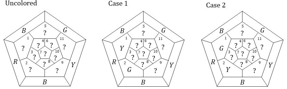
In Figure 2, we have numbered the interior regions of the Errera map. We have also assigned colors to the five regions adjacent to the exterior uncolored region. This can be done without loss of generality, as we can freely rotate the Errera map and permute colors until they are in the configuration shown in Figure 2. It bears mentioning that each of our four colorings of the interior region represents the \(4!\cdot 5=120\) different colorings that can be obtained by permutation and rotation.
We begin with two cases: The regions \(1\) and \(2\) are colored \(Y\) and \(G\) respectively, or the regions \(1\) and \(2\) are colored \(G\) and \(Y\) respectively.
We begin with a general observation that will assist in narrowing down possible impasse colorings.
Observation 3.1. Neither region \(6\) nor region \(10\) can be colored \(R\).
Proof. In an impasse coloring, there must be an \(RY\) circuit. This means that region \(9\) or region \(11\) must be colored \(R\). Since region \(10\) is adjacent to both region \(9\) and region \(11\), it may not be colored \(R\). A similar argument except with the \(RG\) circuit shows that region \(6\) cannot be colored \(R\). ◻
We now proceed to our cases.
In this case, regions \(1\) and \(2\) are colored \(Y\) and \(G\) respectively. We now consider the location of the next \(R\) region in the \(RY\) circuit. Before we do, let us observe a fact that applies to all colorings in Case 1.
Observation 3.2. In Case 1, neither region \(4\) nor region \(8\) can be colored \(R.\)
Proof. If region \(4\) were colored \(R\), then all four colors would be adjacent to region \(5\), and thus region \(5\) could not be colored. This also applies to region \(8\). ◻
Therefore, we see that the next region in the \(RY\) circuit must be either region \(5\) or region \(3\). These will be Cases 1.1 and 1.2, as shown in Figure 3.
In Figure 3, the remainder of the graph for Case 1.1 is colored as well. Starting with just regions \(1, 2,\) and \(5\) colored, we see that the only region adjacent to \(5\) that is not adjacent to another \(Y\) region is \(6\). Due to the \(R\) in region \(5\) and Observation 3.1, the next \(R\) region must be region \(7\). The only region adjacent to \(7\) that is not also adjacent to a \(Y\) is \(8\), which must be the next region in the \(RY\) circuit. Similarly, the only region adjacent to \(8\) that is not adjacent to an \(R\) is region \(9\). This completes the \(RY\) circuit, and regions \(1,2,5,6,7,8,\) and \(9\) have been colored. Region \(3\) is now adjacent to three different colors and must therefore be colored the fourth color, \(B\). The same applies to region \(11\), and then also to regions \(4\) and \(10\) which must be colored \(G\). Thus, this starting coloring of regions \(1, 2,\) and \(5\) determines the remainder of the coloring.
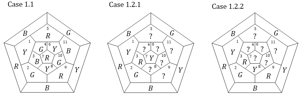
In Case 1.2, there are once again two different places where the next region of the \(RY\) circuit may be located: region \(7\) or region \(8\). These are divided into Cases 1.2.1 and 1.2.2. One can quickly deduce by Observations 3.1 and 3.2 that Case 1.2.1 cannot lead to an impasse coloring of the Errera map. Therefore, we turn our attention to Case 1.2.2. Note that region \(9\) has been colored \(R\), due to the \(R\) in region \(3\) and Observation 3.1. This completes the \(RY\) circuit. Now we turn our attention to the \(RG\) circuit. The next \(G\) region in the \(RG\) circuit may be placed in either region \(4\) or \(7\), giving cases 1.2.2.1 and 1.2.2.2 depicted in Figure 4.
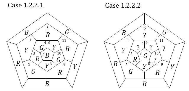
Once again, an entire coloring for Case 1.2.2.1 has been provided. Given colorings of regions \(1,2,3,4,8,\) and \(9\), we see that region \(5\) is adjacent to three different colors (and in fact, has been in all of Case 1) and must be colored \(R\). Region \(7\) is also adjacent to three colors, and therefore must be colored \(B.\) Now region \(6\) is adjacent to three colors and must be colored \(Y\), then similarly region \(11\) must be colored \(B\), and region \(10\) must be colored \(G\). Thus, the remainder of the coloring is determined.
In Case 1.2.2.2, we deduce as in Case 1.2.1 by Observations 3.1 and 3.2 that we cannot have an impasse coloring of the Errera map. Thus, we have completed our examination of Case 1, resulting in only two potential impasse colorings of the Errera map.
In this case, regions \(1\) and \(2\) are colored \(G\) and \(Y\) respectively. Again, we try to complete the \(RY\) circuit. First, we make an observation slightly different than those preceding.
Observation 3.3. In Case 2, neither region \(5\) nor region \(9\) can be colored \(R\).
Proof. Let \(c\) be an impasse coloring in Case 2. Note that since \(c\) is in impasse, there is an \(RY\) circuit, and therefore there is no Kempe chain from the \(B\) boundary region counterclockwise to the vertex to the \(G\) boundary region. If region \(5\) was colored \(G\) in a coloring \(c\), then the left-hand chain (a \(BY\) chain) would consist of only the boundary region clockwise to the vertex. Therefore, \(\alpha(c)\) would have the \(G\) boundary region as its vertex, and there would still be an \(RY\)-chain stretching from the \(R\) boundary region to the \(Y\) boundary region clockwise to the vertex. Therefore, \(\alpha(c)\) could not have a left-hand circuit (which in this case is a \(BG\) circuit), which contradicts that \(c\) is at impasse. The case for region \(9\) is similar. ◻
With this result in hand, we attempt to continue the \(RY\) circuit. Considering Observation 3.3, the next \(R\) region can either be in region \(3\) or \(8\). These are Cases 2.1 and 2.2 in Figure 5, with Case 2.1 divided into two smaller cases.
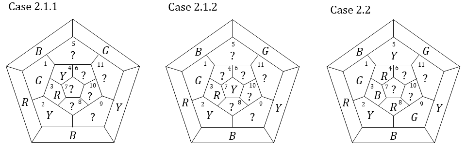
Neither Case 2.1.1 nor Case 2.1.2 can lead to an impasse coloring of the Errera map. In Case 2.1.1, the \(R\) in region \(3\) and Observations 3.1 and 3.3 eliminate all options for the next \(R\) region in the \(RY\) circuit. Similarly, in Case 2.1.2 the \(R\) in region \(3\) and Observation 3.1 eliminate all options for the next \(R\) region. Therefore, we turn our attention to Case 2.2. Once again, some additional regions have been colored. Given colorings of regions \(1,2,\) and \(8\), we see that regions \(3\) and \(9\) are adjacent to three colors and must be colored \(B\) and \(G\) respectively. We also note that the next \(R\) in the \(RG\) circuit cannot be in region \(5\) by Observation 3.3, and thus must be in region \(4\). Now region \(5\) is also adjacent to three colors and must be colored \(Y\).
The next \(Y\) region of the \(RY\) circuit can then be in either region \(7\) or \(10\). These will be Cases 2.2.1 and 2.2.2 in Figure 6. In each case, a complete coloring of the interior regions of the Errera map is determined.
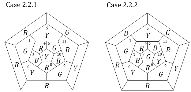
In Case 2.2.1, we start with a coloring of regions \(1,2,3,4,5,7,8,\) and \(9\). Then region \(10\) is now adjacent to three colors and must be colored \(B\). This then causes regions \(6\) and \(11\) each to be adjacent to three colors, and therefore they must be colored \(G\) and \(R\) respectively. Therefore a coloring has been determined. In Case 2.2.2, we again start with a coloring of regions \(1,2,3,4,5,7, 8,\) and \(9\). This time, region \(6\) is adjacent to three colors and must be colored \(B\). This then causes regions \(10\) and \(11\) to be adjacent to three colors, and therefore they must be colored \(Y\) and \(R\) respectively.
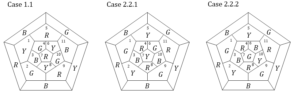
Thus we have completed our analysis of cases. The only cases which potentially provide impasse colorings of the Errera map are Cases 1.1, 1.2.2.1, 2.2.1, and 2.2.2. Note that the coloring in Case 1.2.2.1 is the same as that in Figure 1. We present again the remaining three colorings in Figure 7.
Thus far, we have narrowed our search to four colorings of the interior regions of the Errera map which may have impasse colorings. We have neither shown that these are impasse colorings, let alone colorings having the same cyclic pattern as the coloring \(c_0\) in Figure 1. However, we are aided by the following observation:
Observation 4.1. Let \(c\) be a coloring of the interior regions of the Errera map such that \(\alpha^n\) is at impasse for all \(n\), and \(\alpha^{20}(c)=c.\) Then this is also true for all colorings \(\alpha^k(c),\) for any \(k\).
If we can show that each of the colorings in Figure 7 is \(\alpha^k(c_0)\) for some \(k\), perhaps under some rotation and permutation of colors, then this will show that the coloring is at impasse and has the same cyclic pattern as the original Errera map.
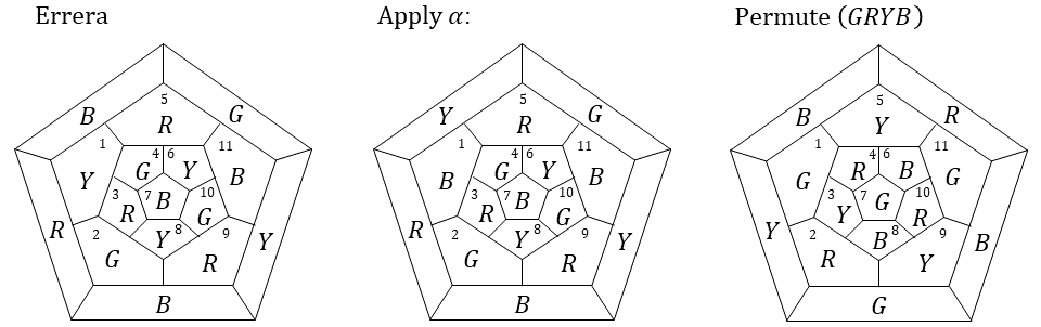
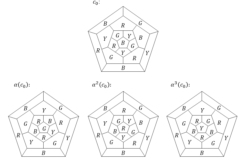
First, we apply \(\alpha\) to the coloring \(c_0\) in Figure 1 and permute the colors by \((GRYB)\). This is shown in Figure 8. We note that this is a rotation of the coloring in Case 2.2.2. Therefore, the coloring in Case 2.2.2 is equivalent to \(\alpha(c_0)\).
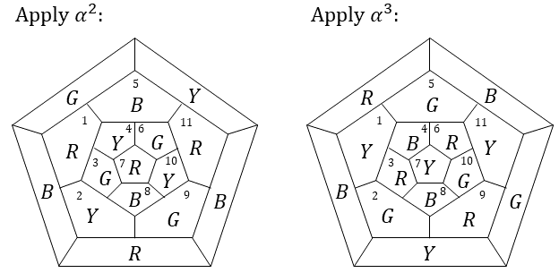
We will now applying \(\alpha^2\) and \(\alpha^3\) to \(c_0\), permuting colors appropriately. These results are given in Figure 9, with the colorings being rotations of Cases 1.1 and 2.2.1 respectively.
We have now described all impasse colorings of the Errera map, which happen to also be colorings leading to a cyclic pattern. This has of course assumed that the uncolored region is one of the pentagonal regions adjacent to no hexagons. Some pentagonal regions of the Errera map are adjacent to hexagons, although these will not be studied here.
We can neatly summarize our findings in the theorems below. For the sake of brevity here and later, we will say that \(R\) is a central pentagon of the Errera map if it is a pentagonal region whose neighbors are also pentagonal regions. We will assume in the following that the Errera map is drawn so that the exterior region is a central pentagon.
Theorem 4.2. Let \(G\) be the Errera map drawn so that the exterior region is a central pentagon, let \(c\) be a proper coloring of the interior regions of \(G\), and let \(c_0\) be the coloring in Figure 1. Then the following are equivalent:
1. \(c\) is an impasse coloring.
2. \(c\) is equivalent to \(c_0, \alpha(c_0), \alpha^2(c_0),\) or \(\alpha^3(c_0)\), possibly under some rotation and/or permuation of colors.
3. \(\alpha^n(c)\) is at impasse for all \(n\), with \(\alpha^{20}(c)=c\).
Corollary 4.3. Let \(G\) be the Errera map drawn so that the exterior region is a central pentagon. There are exactly \(480\) proper colorings of the interior regions of \(G\) that are at impasse, counting rotations and permutations as separate colorings.
We end this section by presenting in Figure 10 all four impasse colorings of the Errera map (up to rotation and permutation of colors). Note that the interior central pentagon of each is colored differently, which makes it easier to distinguish which coloring is present in a given instance.
Now that we have succinctly described all possible impasse colorings of the interior regions of the Errera map, we can briefly discuss how to resolve impasses in all such cases.
The following observation is made by Kittell in [7].
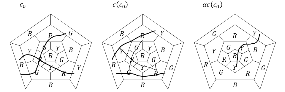
Observation 5.1. Let \(c_0\) be the coloring of the Errera map in Figure 1. Then \(\epsilon(c_0)\) is not at impasse.
Figure 11 demonstrates this to be true. While there are certainly some paths that appear to cross, the existence of at least one \(RY\) circuit and one \(RG\) circuit that do not cross is enough to demonstrate that the coloring is not at impasse by the traditional definition. By our revised definition, we note that \(\alpha\epsilon(c_0)\) does not have a left-hand circuit, and therefore \(\gamma\alpha\epsilon(c_0)\) has only three colors in boundary regions.
One may notice that \(c_0\) and \(\alpha^2(c_0)\) are very similar. In fact, we can observe the following (leaving verification to the reader).
Observation 5.2. Let \(c_0\) be the coloring of the Errera map in Figure 1. Then \(\epsilon(\alpha^2(c_0))\) is not at impasse.
One more observation of Kittell’s will be useful.
Observation 5.3. Let \(c_0\) be the coloring of the Errera map in Figure 1. Then \(\alpha^4(c_0)\) is a rotation of \(c_0\).
This should not be surprising, as \(c_0, \alpha(c_0), \alpha^2(c_0),\) and \(\alpha^3(c_0)\) make up all the distinct impasse colorings of the Errera map. Given our characterization of the impasse colorings of the Errera map and these observations, we can now characterize resolutions of impasse in the Errera map.
Theorem 5.4. Let \(G\) be the Errera map drawn so that the exterior region is a central pentagon, and let \(c\) be a proper coloring of the interior regions of \(G\) which is at impasse. Then the impasse can be resolved by either \(\epsilon\) or \(\epsilon\alpha\).
Proof. By Theorem 4.2 we may assume that \(c\) is \(\alpha^n(c_0)\) for \(0\le n \le 3\). By Observations 5.1 and 5.2 we have handled the cases \(n=0,2\). For \(n=1,3,\) note that applying \(\epsilon\alpha\) to \(\alpha(c_0)\) and \(\alpha^3(c_0)\) results in \(\epsilon\alpha\alpha(c_0)=\epsilon\alpha^2(c_0)\) and \(\epsilon\alpha\alpha^3(c_0)\simeq\epsilon(c_0),\) neither of which is at impasse. Thus we have handled all cases. ◻
Suppose we are four-coloring the regions of a cubic map one-by-one, and upon attempting to assign a color to a region we find it has five colored neighbors using all four colors. It is possible that this graph contains a cycle \(C\) such that the map induced by all regions interior to the cycle is the Errera map (in a way which will be more precisely defined later), with the region currently trying to be colored corresponding to a central pentagon. In such a case, can the findings above translate to a method to assign a color to this region?
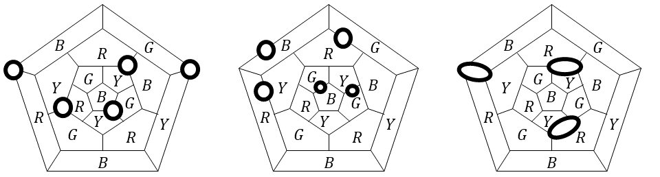
First, let us rephrase this condition in a few ways. First, we may as well exchange “inside” with “outside,” so that all of the regions not belonging to the Errera map are interior to the cycle \(C\). Next, we will say a cubic map is the Errera map with a hole if there is a cycle \(C\) containing any number of regions such that the graph formed by contracting the cycle and all regions interior of the cycle to a vertex is isomorphic to either the Errera map or a bisection of the Errera map. Note that the case where the contraction is a bisection of the Errera map can be ignored, as the dual of such a graph is in fact a multigraph, which can be replaced by a simple graph. We may also allow the Errera map to have more than one hole. Examples of Errera maps with holes, as well as cycles which would not count as holes in this sense, are depicted in Figure 12.
So how many of the results of the previous section translate to the Errera map with holes? The answer is nearly all of them.
Consider a partial coloring of an Errera map with holes. Suppose we would like to assign a color to an uncolored region with at most five colored regions which, after contraction of all holes and vertices of degree \(2\), is a central pentagon of the Errera map. For brevity, we will refer to such a region simply as a central pentagon, even though it or its neighbors may not be pentagons prior to contraction. Further assume that this central pentagon is drawn as the exterior region. Assume also that the only colored neighbors of the exterior region are those on the Errera map proper (that is, no colored region of a hole touches the exterior region). We will make the following observations, with justification where necessary.
Observation 6.1. Adding holes preserves adjacency relations of the Errera map.
Observation 6.2. A proper partial coloring of the Errera map with holes induces a proper partial coloring of the Errera map.
The following fact takes some justification.
Proposition 6.3. The \(AB\) Kempe chains of a partially colored Errera map with holes containing at least one region of the Errera map induce \(AB\) Kempe chains on the induced partial coloring of the Errera map, and vice versa.
Proof. Let \(\mathcal{K}\) be the collection of Kempe chains of the Errera map with holes containing at least one region of the Errera map, and let \(\mathcal{K}'\) be the collection of Kempe chains of the Errera map. First, note that the partial coloring of the Errera map with holes induces a proper partial coloring on the Errera map. Therefore, a Kempe chain \(K\in \mathcal{K}\) contains one or more Kempe chains \(K_1', K_2',…K_t'\in \mathcal{K}'.\) We will show \(K\) contains only a single such Kempe chain.
Suppose to the contrary that there are \(t\ge 2\) Kempe chains of the Errera map contained in \(K\) as described above. Then the regions connecting these Kempe chains must belong to holes. Let \(H\) be a hole connecting at least two distinct Kempe chains \(K_i'\) and \(K_j'\). Then there are regions \(R_i'\) and \(R_j'\) of \(K_i'\) and \(K_j'\) respectively that are both adjacent to regions inside \(H\). Note that all regions bordering \(H\) form a cyclic sequence of adjacent regions in the Errera map. Therefore, since \(R_i', R_j'\) are both bordering \(H\), they are connected by a path through bordering regions along the boundary of H. Thus the Kempe chains \(K_i'\) and \(K_j'\) are connected. This is a contradiction, and the Kempe chain \(K\in \mathcal{K}\) induces exactly one Kempe chain \(K'\in \mathcal{K}'.\)
Thus we have defined a map \(f:\mathcal{K}\rightarrow \mathcal{K}'\) from a Kempe chain in the Errera map with holes to its induced Kempe chain in the Errera map. Since every Kempe chain \(K'\in \mathcal{K}'\) is a subgraph of exactly one Kempe chain \(K\in \mathcal{K}\) (certainly not multiple disconnected Kempe chains, as they must share all regions of \(K'\) in common, contradicting disconnectivity), we also have an inverse \(f^{-1}:\mathcal{K}'\rightarrow \mathcal{K}.\) Thus, we have shown a bijection between the \(\mathcal{K}\) and \(\mathcal{K}'.\) ◻
Next we would like to make an observation about performing Kittell’s color exchange operations on a partially colored Errera map with holes. However, we will now need to modify our definitions slightly to accomodate additional uncolored regions. First, we will always be interested in attempting to assign a color to a specific uncolored region \(R\), which has at most \(5\) colored neighbors, all belonging to the Errera map. We will assume that \(R\) is the exterior region, and \(R\) will take the place of the single uncolored region in our previous definitions. Also, when counting regions clockwise and counterclockwise from a given colored boundary region, we ignore any uncolored regions. If the boundary of a region is interrupted by a hole, as in the second graph in Figure 12, then we ignore the (by necessity uncolored) boundary regions in the hole and count the interrupted region as a single region. Lastly, it might be in the general case that the boundary regions having the same color are consecutive but separated by uncolored regions. Since adjacency is preserved by adding holes this will not be the case here; however, a resolution to such a situation is provided in [3].
We next observe the following, with proof.
Observation 6.4. Let \(c\) be a partial coloring of an Errera map with holes, let \(c'\) be the induced coloring of the Errera map, and let \(\sigma\) be a color exchange operation. Then the proper coloring \(\sigma(c)\) induces the proper coloring \(\sigma(c')\) on the Errera map.
Proof. Let \(K\) be a Kempe chain in the Errera map with holes that begins at a colored boundary region. Such a region necessarily belongs to the Errera map, and thus this induces a Kempe chain \(K'\) on the Errera map beginning at that same region. Then, \(\sigma(c)\) exchanges the colors on \(K\). This induces a proper coloring of the Errera map without holes, where the colors on \(K'\) have been exchanged. This is exactly \(\sigma(c').\) ◻
These observations culminate in the following theorem about impasse in the Errera map with holes.
Theorem 6.5. A partial coloring of the Errera map with holes is at impasse if and only if the induced coloring of the Errera map is also at impasse.
Proof. Let \(c\) be a partial coloring of the Errera map with holes, and \(c'\) be the induced partial coloring of the Errera map. First, suppose \(c\) is at impasse. Then \(c\) has a left-hand circuit and right-hand circuit. Since these are Kempe chains starting at colored boundary regions, and all colored boundary regions are also boundary regions of the Errera map, this induces left-hand and right-hand circuits in \(c'\). If \(c\) is at impasse, \(\alpha(c)\) and \(\beta(c)\) each have a left-hand circuit and a right-hand circuit. These induce colorings which also have left-hand and right-hand circuits; by Observation 6.4, these colorings are exactly \(\alpha(c')\) and \(\beta(c')\). Therefore \(c'\) is at impasse.
For the reverse direction, suppose that \(c'\) is at impasse. Then \(\alpha(c)\) and \(\beta(c)\) induce colorings \(\alpha(c')\) and \(\beta(c')\). Since \(c'\) is at impasse, \(c', \alpha(c'),\) and \(\beta(c')\) each have left-hand and right-hand circuits. These circuits are each subgraphs of left-hand and right-hand circuits in \(c, \alpha(c)\), and \(\beta(c)\) respectively. Thus, \(c\) is also at impasse. ◻
As a result of Theorem 6.5, most of our previous results follow. If the Errera map with holes is at impasse, then the induced coloring of the Errera map is also at impasse. Applying \(\alpha\) any number of times will still result in an impasse coloring of the Errera map, which translates to an impasse coloring of the Errera map with holes. However, while applying \(\alpha^{20}\) returns the coloring of the Errera map to its original impasse coloring, the same is not necessarily true of regions inside holes. However, since the number of colorings is finite and applying \(\alpha\) repeatedly does not resolve the impasse, it follows that the sequence of partial colorings generated by \(\alpha\) will also be cyclic with some period \(p\) such that \(20 | p\).
Of most interest is the fact that, since we can resolve all impasse colorings of the Errera map, we can also resolve all impasse colorings of the Errera map with holes.
Theorem 6.6. Let \(G\) be an Errera map with holes, and let \(c\) be a partial coloring of \(G\), where all regions of the Errera map except for a central pentagon \(R\) have been assigned a color. Suppose further that the only colored neighbors of \(R\) belong to the Errera map, and when attempting to assign a color to \(R\), the coloring \(c\) is at impasse. Then the impasse can be resolved by either \(\epsilon\) or \(\epsilon\alpha\).
We begin by exhibiting in Figure 13 an example of an Errera map with a hole. This graph was generated randomly using the reduction algorithm described by Morgenstern and Shapiro in [8]. Specifically, this was generated as a maximal planar graph, then converted to a cubic map. The regions of the map have been carefully arranged to make its structural properties apparent.
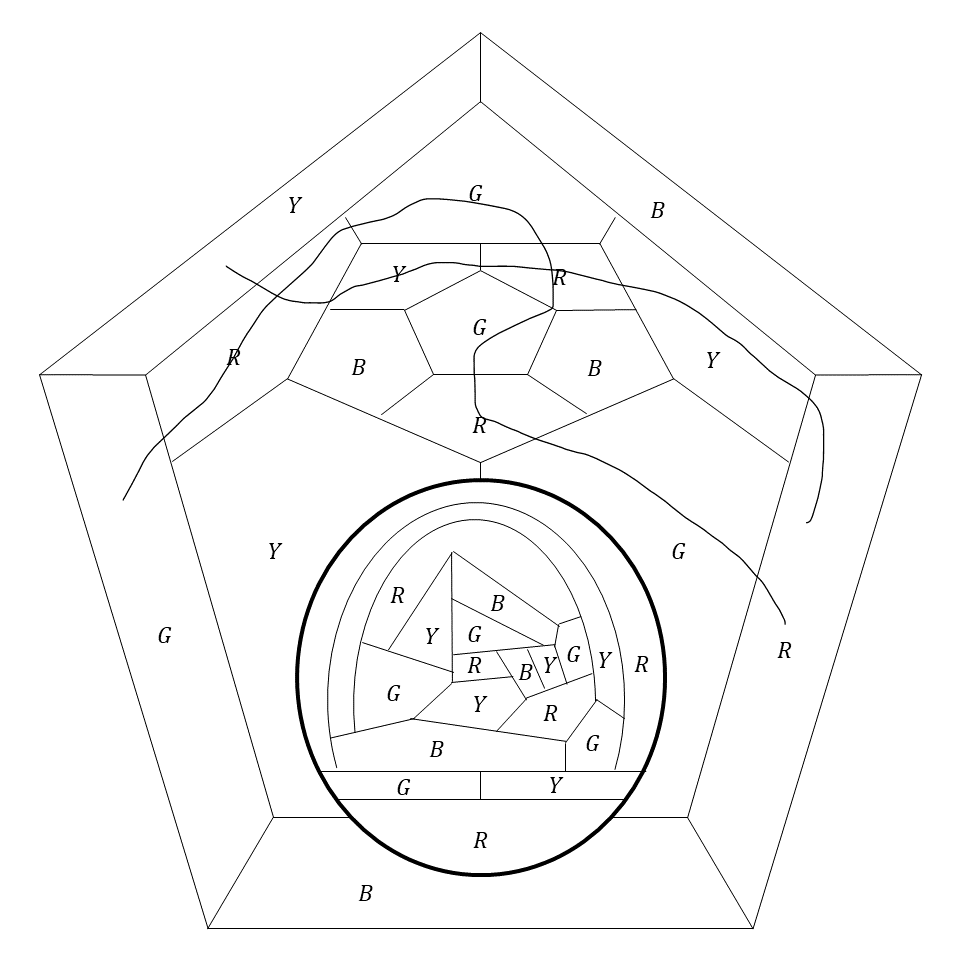
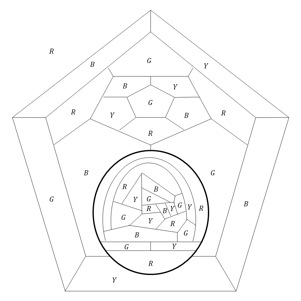
We will note that it takes \(60\) applications of \(\alpha\) to return this graph to its original coloring (leaving verification to the reader). We can also observe by the fact that the interior central pentagon is colored \(G\) that the induced coloring of the Errera map is a rotation of \(\alpha(c_0)\). Therefore, we should be able to resolve the impasse by \(\epsilon \alpha\) and furthermore obtain only three colors on the boundary regions by next applying \(\gamma\alpha.\) In Figure 14 we show the coloring obtained by applying \(\gamma\alpha\epsilon\alpha\) to the map in Figure 13. At this point, the exterior region can be colored \(R\), obtaining a coloring of all regions of the map.
One may wonder why Errera maps with holes are of particular interest. On one hand, we have seen that certain partial colorings of Errera maps with holes are at impasse under repeated application of \(\alpha,\) showing that this entire class of graphs is rather troublesome. On the other hand, we have now developed a method of resolving impasses in these troublesome cases with only a handful of color exchanges. More compellingly, there is some preliminary experimental evidence to suggest that these are the only situations where repeated application of \(\alpha\) fails to resolve the impasse. If this could be proven to be true, then this would be an alternate proof of the Four Color Theorem, and further an answer in the affirmative that every impasse can be resolved by a sequence of Kempe color exchanges. Even if this is not true, a counterexample would be very instructive to study more closely.
The data that support the findings of this study are available from the corresponding author upon reasonable request.
On behalf of all authors, the corresponding author states that there is no conflict of interest.