A block graph is a graph in which every block, or maximal biconnected subgraph, is a complete graph [6]. Equivalently, it can be described as a tree of cliques, where the blocks are complete subgraphs interconnected in a tree-like structure. According to Harary’s definition [6], the vertices of a block graph represent either the original vertices of the graph or the blocks themselves. Any cut-vertex of a block graph belongs to at least two blocks, as it is responsible for the maintenance of connectivity between them. The block graphs are also chordal, meaning they have no induced cycles of length more than three, and they are perfect, where every induced subgraph has a chromatic number equal to the size of its largest clique.
In an electric power network, redundancy is critical to the tolerance of failure. Block graphs thus represent fault-tolerant systems with strongly interconnected local components that form complete graphs representing the connections between them that, if one fails, ensures that the network remains active. This is a representation of substation and transmission line blocks, where engineers can take the effect of local failures like a substation outage in a system and find an alternative path for power flow because there are multiple blocks.
For instance, neighbourhoods (blocks) can act as self-contained micro-grids (complete graphs) in a smart grid, and the interconnection via critical substations or transmission lines (cut-vertices) constitutes the block graph. If some neighborhoods fail, they can work individually. Repair activities can focus on making the substations or lines critical to connect again. With this background, block graphs provide a solid conceptual as well as computational approach towards designing, analyzing, and optimizing resilient and efficient power networks.
The following definitions from [6] set up the terminologies and concepts that will be important in the discussions of the rest of this article: A graph \(G = (V, E)\) consists of a set of vertices \(V\) and a set of edges \(E\), where every edge is an unordered pair of distinct vertices. Graphs can be used for modeling relations and connections between different entities in systems. A cut vertex in a connected graph \(G\), is a vertex such that the removal of which increases the number of connected components of \(G\). It is a key node that ensures connectivity. A graph or subgraph is biconnected if it is connected and remains connected after the removal of any single vertex. Biconnected graphs do not have cut vertices, and every edge lies on at least one cycle. A block of a graph is a maximal biconnected subgraph. Blocks are the largest subgraphs of \(G\) such that removing any vertex does not render the subgraph disconnected. A graph has an intrinsic block decomposition, and this decomposition is unique. A clique in a graph is defined as a subset of vertices such that every two distinct vertices in the subset are adjacent. That is, a clique is a complete subgraph where all vertices are directly connected. A tree is an acyclic connected graph. In a tree, any two vertices are connected by just one path, and for any edge, its removal disconnects the graph. A pendant vertex (or leaf) is a vertex of degree one in a graph. It is connected to the rest of the graph by a single edge.
The concept of power domination in graphs originates from the need to monitor electric power networks effectively, as introduced by Haynes et al. in 2002 [7]. The problem can be viewed as a variant of the classical domination problem, where certain propagation rules mimic the flow of information in network monitoring.
Formally, a Power Dominating Set (PDS) of a graph \(G\) is a subset \(S \subseteq V\) of vertices such that all vertices in the graph are either in \(S\) or can be monitored by the vertices in \(S\) according to specific propagation rules. These rules are inspired by the behavior of power networks where placing a minimum number of phasor measurement units (PMUs) ensures the observability of the entire system.
All vertices in \(S\) (the power dominating set) are initially marked as monitored.
Any neighbors of vertices in \(S\) are marked as monitored.
If a monitored vertex has exactly one unmonitored neighbor, that neighbor becomes monitored.
This process continues iteratively until no further vertices can be monitored.
A PDS helps in placing PMUs optimally in a power grid to ensure the entire network’s observability with minimal cost. It also models optimal sensor placement in monitoring systems. Various works have been devoted to developing various methods for optimal PMU placement, including those presented in [1, 3, 2]. The minimum size of a PDS in a graph graph \(G\) is called its power domination number (\(\gamma_P(G)\)) [7].
The \(k\)-fault tolerant power domination problem extends this concept to account for the failure of up to \(k\) vertices in the graph. This extension is particularly relevant in real-world scenarios, where systems need to remain functional despite failures. Formally, a set \(S \subseteq V\) is referred to as a \(k\)-fault tolerant power dominating set [8] of a given graph \(G\) if the difference \(S \backslash F\) remains a power dominating set of \(G\) for any \(F \subseteq S\) with \(|F| \leq k\), where \(k\) is an integer with \(0 \leq k < |V|\). The lowest cardinality of a \(k\)-fault tolerant power dominating set is the \(k\)-fault tolerant power domination number of \(G\), denoted by \(\gamma_P^k (G)\). The \(k\)-fault tolerant power domination problem seeks to determine \(\gamma_P^k(G)\) and identify the corresponding set, representing the minimum number of PMUs required to monitor a system reliably, even in the presence of up to \(k\) faults. Several studies have addressed this problem for specific classes of graphs. For instance, Lakshmi and Somasundaram [5] determined the \(k\)-fault-tolerant power domination number for generalized Petersen graphs and cylinders, while Dorfling and Henning [4] investigated power domination in grid graphs. Building on these efforts, the present study aims to extend the understanding of \(k\)-fault tolerant power domination to block graphs, providing new insights into the placement of PMUs under fault-prone conditions.
In order to present our observation clearly, we introduce the following definitions on a block graph \(G\).
Definition 3.1(Hanging paths of a block graph).Let \(v\) be a vertex in the PDS of the block graph \(G\). Consider all the blocks of size 2 that contain the vertex \(v\), that initiates a path \(v – a_1 – a_2 – a_3 \cdots\) such that each vertex except \(v\) mentioned here in the path has degree exactly two, except for the last vertex, which has degree one. Such paths are called hanging paths of vertex \(v\).
Definition 3.2. We define \(l_{HP}(va_1a_2\cdots)\) as the length of the hanging path starting at \(v\) such that all internal vertices in the path (excluding \(v\)) have degree two, and the terminal vertex has degree exactly one.
Definition 3.3. Let \(l_i(HP_v)\) be defined as the length of the \(i^{\text{th}}\) smallest hanging paths of \(v\).
Definition 3.4. Define \(K_v\) as the minimum of sizes of blocks of graph \(G\) containing the vertex \(v\) (excluding the ones with size two) and \(l_1(HP_v) + l_2(HP_v)\).
To effectively state and prove our results, we introduce partitioning of specific sets. To begin with consider \(S\) be a power dominating set of \(G\) such that each vertex of \(S\) is a cut-vertex. This is possible due to Lemma 2.1 of [9].
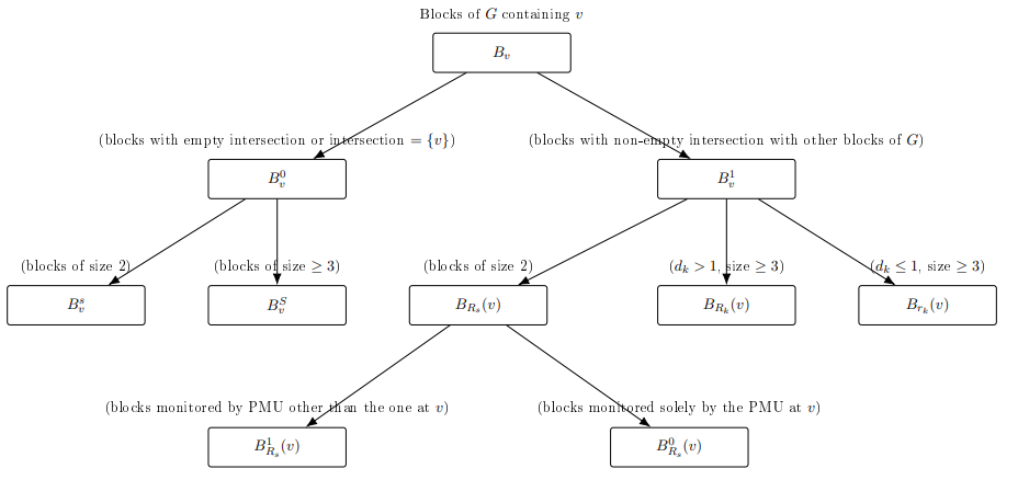
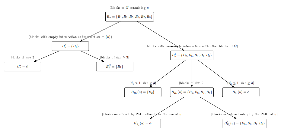
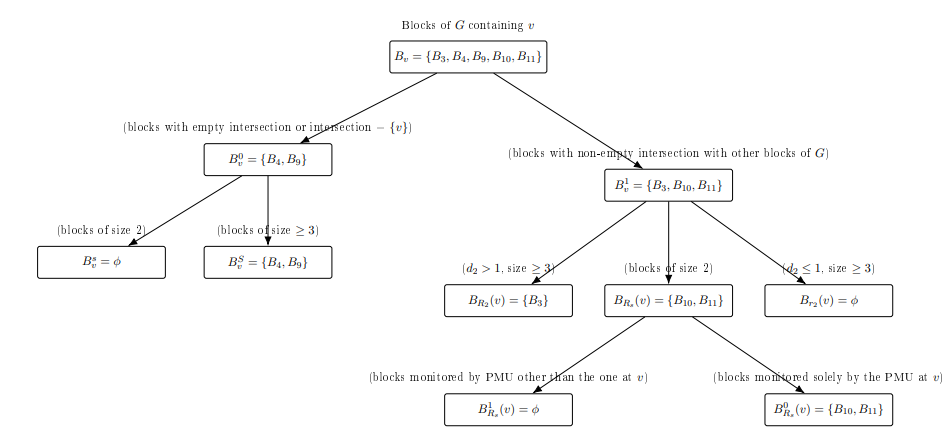
\(B_v\): The set of all blocks (maximal biconnected subgraphs, i.e., cliques) in \(G\) that contain the vertex \(v\).
Bipartition of \(B_v\): \[B_v = B_v^0 \cup B_v^1,\] where \(B_v^0\) and \(B_v^1\) are disjoint subsets.
\(B_v^0\) consists of blocks that intersect only at \(v\) or have empty intersection with other blocks.
\(B_v^1\) consists of blocks intersecting with other blocks in vertices other than \(v\).
Further partition of \(B_v^0\): \[B_v^0 = B_s^v \cup B_S^v,\] where:
\(B_s^v\) contains blocks of size 2 (edges) that contain \(v\).
\(B_S^v\) contains blocks of size greater than two (cliques of size \(\geq 3\)) that only intersect other blocks at \(v\).
Tripartition of \(B_v^1\): \[B_v^1 = B_{r_k}(v) \cup B_{R_k}(v) \cup B_{R_s}(v),\] three mutually exclusive subsets:
\(B_{R_s}(v)\): Blocks of size 2 in \(B_v^1\).
\(B_{r_k}(v)\): Blocks of size \(\geq 3\) with \(d_k \leq 1\)
\(B_{R_k}(v)\): Blocks of size
\(\geq 3\) with \(d_k > 1\)
where \[d_k = \text{size of the block} – c +
k – 2,\] and \(c\) denotes the
number of cut vertices of \(G\)
contained in the blocks of \(B_v^1\)
that can be monitored by the PMUs placed at the vertices of \(S\), excluding the one located at vertex
\(v\).
Bipartition of \(B_{R_s}(v)\): \[B_{R_s}(v) = B_{R_s}^0(v) \cup B_{R_s}^1(v),\] where:
\(B_{R_s}^0(v)\) are blocks monitored solely by the PMU at \(v\).
\(B_{R_s}^1(v)\) are blocks monitored by PMUs other than at \(v\).
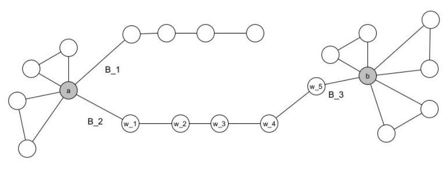
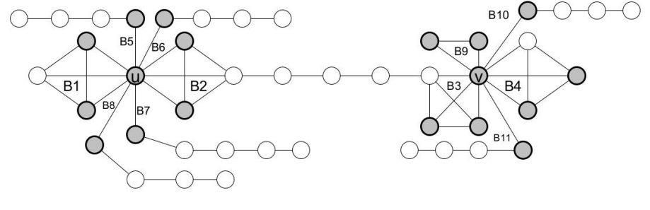
To illustrate the distinction between \(B_{R_s}^0(v)\) and \(B_{R_s}^1(v)\), consider the vertex \(w_1 \in B_2\) of the graph in Figure 1. This vertex in block \(B_2\) is monitored by the PMUs placed at vertices \(a\) and \(b\). Specifically, vertex \(a\) directly dominates \(w_1\), while vertex \(b\) dominates \(w_5\). The monitoring effect from \(b\) then propagates sequentially through the vertices \(w_5 \rightarrow w_4 \rightarrow w_3 \rightarrow w_2 \rightarrow w_1\). Consequently, \(w_1\) becomes a vertex monitored by both PMUs located at \(a\) and \(b\). A similar observation holds for vertex \(w_5\). In contrast, the vertex in block \(B_1\), other than the vertex \(a\), is monitored solely by the PMU at \(a\). Therefore, \(B_1 \in B_{R_s}^0(v)\) and \(B_2, B_3 \in B_{R_s}^1(v)\).
Set \(B\): \[v \in B \quad \text{if} \quad |B_s^v \cup B_{R_s}^0(v)| \geq 2,\]
This classification helps decide where extra PMUs must be placed for fault tolerance.
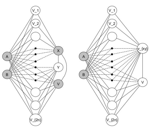
The partitions of the set \(B_v\), for each \(v \in S\), as described above, are illustrated in the following flow chart (Figure 2) for better clarity.
Theorem 3.5. For a block graph \(G\), the \(k\)-fault tolerant power domination number \(\gamma_P^k(G)\) satisfies:
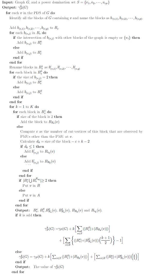
\[\gamma_P^k(G) = \begin{cases} \begin{aligned} &\gamma_P(G) + k \Bigg[\sum_{v \in S} \big( |B_v^S| + |B_{R_k}(v)| \big) \Bigg] \\[4pt] &\quad + \Bigg[\sum_{v \in B} \Big\{ \big( |B_v^s| + |B_{R_s}^{0}(v)| \big) \Big( \dfrac{k+1}{2} \Big) \Big\} – 1 \Bigg], && \text{if } k \text{ is odd}, \\[12pt] &\gamma_P(G) + k \Bigg[\sum_{v \in S} \big( |B_v^S| + |B_{R_k}(v)| \big) \Bigg] \\[4pt] &\quad + \Bigg[\sum_{v \in B} \big( |B_v^s| + |B_{R_s}^{0}(v)| \big) \Big( \dfrac{k}{2} \Big) \Bigg], && \text{if } k \text{ is even}. \end{aligned} \end{cases}\] where \(k\) does not exceed two if any vertex in the PDS of \(G\) has two or more pendant neighbors. Otherwise, \(k < K = \min\limits_{v} K_v\).
Proof. Let \(G\) be a block graph and \(S\) be its minimum power dominating set (PDS) that contains only cut vertices. A PMU placed at a vertex \(v \in S\) directly monitors every block in \(G\) containing \(v\) and further propagation may monitor other vertices too.
Consider the failure of the PMU at a particular \(v \in S\). To ensure \(k\)-fault tolerance, all blocks containing \(v\) must be monitored by other PMUs. However, placing a PMU in just one block containing \(v\) cannot monitor the other blocks of size greater than two because propagation does not extend across these blocks. This necessitates placing \(k\) additional PMUs in each block, of size greater than two, containing \(v\) that uniquely depends on it, captured by the term \(k|B_v^S|\) in the sum.
Special consideration is given to blocks of size two (edges), collected in \(B_v^s\). When all other adjacent blocks are monitored, a size-2 block can be monitored via propagation, since it becomes the unique unmonitored neighbor of \(v\). This behavior justifies the fractional terms involving \(|B_v^s|\) and \(|B_{R_s}^0(v)|\), explaining why for odd and even \(k\), an additional \(\frac{k+1}{2}\) or \(\frac{k}{2}\) PMUs, respectively, suffice to cover these hanging path-like structures.
Next, we justify the inclusion of the term involving \(B_{R_k}(v)\) and \(B_{r_k}(v)\), which measures the redundancy of monitoring within blocks of size at least three. Consider a block \(B \in B_{R_k}(v)\) of size three containing the cut vertex \(v \in S\). Suppose that, apart from \(v\), the block also contains another cut vertex \(w\) of \(G\). When the PMU placed at \(v\) fails, the vertex \(v\) itself will eventually be monitored by PMUs located in the other blocks containing \(v\). Likewise, the vertex \(w\) will remain monitored, as it is already observed by PMUs positioned in other blocks adjacent to \(w\) that belong to \(S\). Consequently, even after failure of the PMU at \(v\), two vertices of this block—namely \(v\) and \(w\)—remain monitored. Since the block is a clique of order 3, the third vertex can be monitored by propagation.
This observation highlights that blocks may vary in their inherent level of redundancy, depending on how many of their vertices remain monitored after failures of PMUs in adjacent articulation points. Hence, for each block in \(B_{R_k}(v)\) and \(B_{r_k}(v)\) we define \(d_k = \text{size of block} – c +k -2\), where \(c\) denotes the number of cut vertices in \(B\) monitored by PMUs other than at \(v\). The value of \(d_k\) quantifies the number of unmonitored vertices in \(B\) after a worst-case failure scenario. When \(d_k \leq 1\), there remains at most one unmonitored vertex in \(B\), which can be subsequently observed through propagation; thus, no additional PMU is necessary. These blocks belong to \(B_{r_k}(v)\). Conversely, when \(d_k > 1\), there exist at least two unmonitored vertices, preventing propagation in the block (since each of the remaining vertices has at least two unmonitored neighbors). In such cases, redundancy cannot be achieved via propagation alone, necessitating the introduction of additional PMUs. These blocks form the set \(B_{R_k}(v)\), and the contribution \(k|B_{R_k}(v)|\) in the right-hand side of the expression accounts for the required backup PMUs for these structurally low-redundancy blocks.
Moreover, if a vertex \(v\) in the PDS has two or more pendant neighbors, it is impossible to construct a \(k\)-fault tolerant PDS for \(k \geq 3\), since PMUs at \(v\) and its pendant neighbors could all fail, leaving those vertices unmonitored.
Thus, the formula accounts for:
the original minimum PDS controls (\(\gamma_P(G)\)),
the number of blocks that require \(k\) backup PMUs due to unique monitoring (\(k \sum_{v} |B_v^S|\\ + |B_{R_k}(v)|\)),
additional PMUs for hanging paths and small blocks \(k\) (\(\sum_{v\in B} (|B_v^s| + |B_{R_s}^0(v)|) \times f(k)\)).
This expression guarantees full observation despite any \(k-\)PMU failures in the network. It also clearly substantiates the minimality of the constructed set, since the construction incorporates only the essential number of additional PMUs required to ensure \(k\)-fault tolerance.
Finally, we justify the choice of \(S\) as the minimum PDS containing only cut vertices. In block graphs, each block is a clique, and power domination initiated at a non-cut vertex effectively monitors the entire block rapidly due to the clique structure. While such a non-cut vertex may additionally monitor small adjacent blocks of size two via propagation, its influence remains largely local to its own block and immediate neighbors. When constructing a \(k\)-fault tolerant power dominating set (\(k\)-FPDS), failure of a PMU at a non-cut vertex necessitates placing additional PMUs at relevant cut vertices connecting other blocks that become unmonitored due to this failure. Conversely, beginning with a minimum PDS consisting solely of cut vertices, failure of a PMU at such a cut vertex requires augmenting the set with backup PMUs within the adjacent blocks, often at non-cut vertices, to maintain fault tolerance.
In both constructions, the total number of PMUs (original plus backups) needed in the \(k\)-FPDS remains essentially the same, as redundancy must address the same structural vulnerabilities, just allocated differently between cut and non-cut vertices. Thus, whether starting from a minimum PDS with non-cut vertices or a minimum PDS of cut vertices, constructing a minimal \(k\)-FPDS leads to the same total PMU count once fault tolerance requirements are met.
This observation substantiates the approach of focusing on minimum cut-vertex PDSs for \(k\)-FPDS construction, as it captures the essential redundancy requirements without increasing the total PMU count. ◻
Adhering to the above explanations, an algorithm to generate a \(k-\)fpds for any block graph \(G\) is provided here.
Example 3.6. Let us now illustrate the application of the theorem 3.5 and the corresponding algorithm. Consider the graph shown below in Figure 3, whose minimum power dominating set is \(\{ u, v \}\). Observe that both \(u\) and \(v\) are cut-vertices.
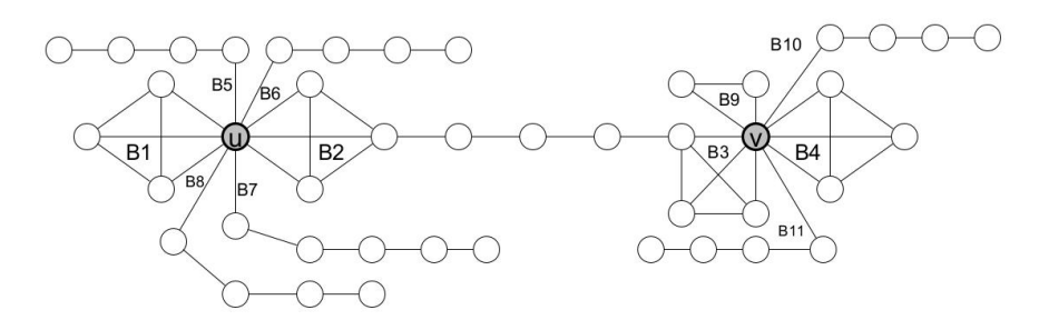
We proceed by following the steps outlined in the algorithm to determine the partitions of the blocks of \(G\) containing \(u\) and \(v\), as depicted in the flowcharts given below in Figure 4 and Figure 5, respectively.
Having obtained these partitions, we then determine the exact cardinality of each partition set. These values can subsequently be substituted into the formula derived in the theorem 3.5, as follows:
\[\begin{aligned} \gamma_P^1(G) =& \gamma_P(G) + \Big[\sum_{v \in S } \Big\{ |B_v^S| + |B_{R_1}(v)| \Big\} \Big] + \Big[\sum_{v \in B } \Big\{ |B_v^s| + |B_{R_s}^0(v)| \Big\} \Big( \frac{1+1}{2} \Big) – 1 \Big]\\ =& 2 + \Big[ 2 + 3 \Big] + \Big[ 4 \Big( \frac{1+1}{2} \Big) – 1 \Big] + \Big[ 2 \Big( \frac{1+1}{2} \Big) – 1 \Big]\\ =& 2 + \Big[ 5 \Big] + \Big[ 4 – 1 \Big] + \Big[ 2 – 1 \Big] = 11 . \end{aligned}\] And \[\begin{aligned} \gamma_P^2(G) =& \gamma_P(G) + \Big[\sum_{v \in S } 2 \Big\{ |B_v^S| + |B_{R_2}(v)| \Big\} \Big] + \Big[\sum_{v \in B } \Big\{ |B_v^s| + |B_{R_s}^0(v)| \Big\} \Big( \frac{2}{2} \Big) \Big]\\ =& 2 + \Big[ 4 + 6 \Big] + \Big[ 4 \Big( \frac{2}{2} \Big) \Big] + \Big[ 2 \Big( \frac{2}{2} \Big) \Big]\\ =& 2 + \Big[ 10 \Big] + \Big[ 4 \Big] + \Big[ 2 \Big] = 18 . \end{aligned}\]
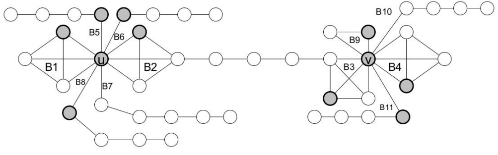
Here, \(K = 3\), as vertex \(v\) belongs to the smallest block of size three (excluding blocks of size two). Consequently, a 3-fault-tolerant power dominating set (3-FPDS) does not exist. In other words, if all PMUs at the vertices of \(B_9\) fail, there are no alternative options to monitor \(B_9\). Figures 6 and 7 depict possible placements of 11 PMUs for a 1-fpds and 18 PMUs for a 2-fpds, respectively.
In this section, we obtained a lower bound for \(k\) fault tolerant power domination number when an edge \(G\) is contracted. This lower bound is tight.
Theorem 4.1. Let \(G\) be a graph, and let \(e = xy\) be an edge in \(G\) with end vertices \(x\) and \(y\). Denote by \(G \circ e\) the contraction of \(e\) in \(G\), and let \(v_{xy}\) be the vertex resulting from contracting \(x\) and \(y\). Then: \[\gamma_P^1(G) – 2 \leq \gamma_P^1(G \circ e).\]
Moreover, there is no general upper bound for \(\gamma_P^1(G \circ e)\) in terms of \(\gamma_P^1(G)\), and the above lower bound is tight for an infinite family of examples.
Proof. Let \(\mathcal{T}\) be a minimum \(1\)‑fault‑tolerant power dominating set (1‑FPDS) of \(G \circ e\). We shall construct from \(\mathcal{T}\) a \(1\)‑FPDS \(\mathcal{S}\) of \(G\) whose cardinality is at most \(|\mathcal{T}| + 2\). This establishes the claimed bound.
Case 1. \(v_{xy} \in \mathcal{T}.\)
Define \(\mathcal{S}_1 = (\mathcal{T} \setminus \{v_{xy}\}) \cup \{x, y\}\). In \(G \circ e\), the PMU placed at \(v_{xy}\) dominates \(N(x) \cup N(y)\) and propgates to atmost one vertex, call it \(v_0\), which is incident to either \(x\) or \(y\) in the graph \(G\). We now verify that \(\mathcal{S}_1\) remains a \(1\)‑FPDS of \(G\) by considering all possible adjacency configurations and fault scenarios.
There are three possible adjacency configurations among \(x, y,\) and a vertex \(v_0 \in N(x) \cup N(y)\) which was reached by propagation in \(G \circ e\).
(a) \(v_0 \in N(x) \text{ but } v_0 \notin N(y)\)
If the PMU at \(x\) fails: The PMU at \(y\) remains and dominates \(x\). All vertices in \(N(x) \setminus \{v_0\}\) are already monitored by the PMUs in \(\mathcal{T} \setminus \{v_{xy}\}\), as in \(G \circ e\). Therefore, \(v_0\) becomes the unique unmonitored neighbor of \(x\), allowing \(x\) to propagate monitoring to \(v_0\) per power domination rules.
If the PMU at \(y\) fails: The PMU at \(x\) remains active and dominates both itself and \(v_0\). Other vertices are already monitored by PMUs in \(\mathcal{T} \setminus \{v_{xy}\}\).
If the PMU at any other vertex of \(\mathcal{S}_1\) fails: Both \(x\) and \(y\) remain active to sustain all domination and propagation operations formerly executed by \(v_{xy}\), ensuring full monitoring.
(b) \(v_0 \in N(y) \text{ but } v_0 \notin N(x)\)
The reasoning mirrors the previous point, with \(x\) and \(y\) roles swapped.
(c) \(v_0 \in N(x) \cap N(y)\)
If either PMU at \(x\) or \(y\) fails, the other continues to dominate \(v_0\) and replicate all propagation steps from \(v_{xy}\). Moreover, when the fault occurs in any \(u \in \mathcal{T} \setminus \{v_{xy}\}\), both \(x\) and \(y\) remain functional, so domination and propagation remain unimpaired.
Hence, for every possible single failure, \(\mathcal{S}_1\) continues to monitor every vertex of \(G\). Therefore, \(\mathcal{S}_1\) is a \(1\)‑FPDS of \(G\) with \(|\mathcal{S}_1| \leq |\mathcal{T}| + 1\).
Case 2. \(v_{xy} \notin \mathcal{T}.\)
In \(G \circ e\), the vertex \(v_{xy}\) is monitored through propagation from some vertex \(w_0 \in \mathcal{T}\). Let \(\mathcal{S}_2 = \mathcal{T} \cup \{x, y\}\).
We must again verify that \(\mathcal{S}_2\) remains a \(1\)‑FPDS of \(G\) by considering all adjacency configurations between \(w_0\) and the endpoints of the contracted edge.
(a) \(w_0 \in N(x) \text{ but } w_0 \notin N(y)\)
Fault at \(x\), \(y\) remains active:
Since \(y\) has a working PMU, it dominates \(x\) and all vertices in \(N(x) \cap N(y)\) and \(N(y)\).
Vertices in the neighborhood of \(x\) remain monitored by vertices in \(\mathcal{T} \setminus \{v_{xy}\}\), replicating the monitoring steps defined in \(G \circ e\).
Fault at \(y\), \(x\) remains active:
PMU at \(x\) continues to dominate both itself, \(w_0\) and \(y\), as well as the neighborhood of \(x\).
All other vertices remain monitored in this configuration by vertices in \(\mathcal{T} \setminus \{v_{xy}\}\), replicating the monitoring steps defined in \(G \circ e\). .
Fault at any other vertex \(u \in \mathcal{T}\):
Working PMUs at both \(x\) and \(y\) monitors \(x\), \(y\), \(w_0\) and \(N(x) \cup N(y)\)
All domination and propagation steps performed by \(v_{xy}\) and \(\mathcal{T} \setminus \{v_{xy}\}\) in \(G \circ e\) are preserved in \(G\) by \(\mathcal{S}_2\) too.
(b) \(w_0 \in N(y) \text{ but } w_0 \notin N(x)\)
The reasoning mirrors the previous point, with \(x\) and \(y\) roles swapped.
(c) \(w_0 \in N(x) \cap N(y)\)
In this case, \(w_0v_{xy}\) in \(G \circ e\) corresponds to both \(w_0x\) and \(w_0y\) in \(G\). If a PMU fails at either \(x\) or \(y\), the other together with \(w_0\) ensures that domination and propagation follow exactly as in \(G \circ e\). When a fault occurs at any vertex \(u \in \mathcal{T}\), both \(x\) and \(y\) remain available and maintain the same overall monitoring via domination and propagation.
Thus, after any single failure—whether at \(x\), \(y\), or any vertex of \(\mathcal{T}\)—the configuration \(\mathcal{S}_2\) continues to dominate and propagate monitoring to every vertex of \(G\). Hence \(\mathcal{S}_2\) is a \(1\)‑FPDS of \(G\) satisfying \(|\mathcal{S}_2| \leq |\mathcal{T}| + 2\).
From both cases, we obtain \(\gamma_P^1(G) \leq \gamma_P^1(G \circ e) + 2\), which gives the lower bound \(\gamma_P^1(G) – 2 \leq \gamma_P^1(G \circ e)\).
The bounds shown in above theorem are tight. We have shown an infinite family of graphs \(G_n\) in Example 4.2 for the tight lower bound.
There is no upper bound for \(\gamma_P^1(G \circ e)\) in terms of \(\gamma_P^1(G)\), as shown in Example 4.3. ◻
Example 4.2. A family \(G_n\) showing a sharp lower bound.
Consider the graph \(G_n\) with \(2n + 5\) vertices constructed as follows:
\(V(G_n) = \{ A, B, X, Y, v , v_1, v_2, \cdots , v_{2n} \}\)
\(N(X) = \{ v_1, \cdots, v_n \}\)
\(N(Y) = N(v) = \{v_{n+1}, \cdots, v_{2n}\}\)
Also, we have \(XY, Xv \in E(G_n)\)
For this family \(G_n\), illustrated in Figure 8, the following holds:
\(\gamma_P(G_n) = 2\) with minimum PDS \(\{A, Y\}\).
\(\gamma_P^1(G_n) = 4\) with 1-fault-tolerant power dominating set \(\{A, B, X, Y\}\).
After contracting edge \(X Y\) to form \(G_n \circ XY\):
\(\gamma_P(G_n \circ XY) = 1\) with minimum PDS \(\{A\}\).
\(\gamma_P^1(G_n \circ XY) = 2\) with 1-fault-tolerant power dominating set \(\{A, B\}\).
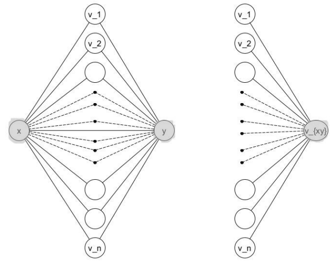
Example 4.3. A family \(G_n\) showing unbounded upper bound.
Consider the graph \(G_n\) with \(n + 2\) vertices constructed as follows:
\(V(G_n) = \{x, y, v_1, v_2, \ldots, v_n\}\)
Each of \(v_i\) (for \(1 \leq i \leq n\)) is adjacent to both \(x\) and \(y\); thus, \(N(x) = N(y) = \{v_1, v_2, \ldots, v_n\}\)
The edge \(xy\) also belongs to \(E(G_n)\).
For this family \(G_n\), illustrated in Figure 9, the following hold:
The minimum power dominating set (PDS) of \(G_n\) is \(\{x\}\) (or symmetrically \(\{y\}\)): the PMU at \(x\) dominates \(y\) and all \(v_i\) through domination.
The minimum 1-fault-tolerant power dominating set (1-FPDS) of \(G_n\) is \(\{x, y\}\): each vertex can compensate for the failure of the other, ensuring that all \(v_i\) remain monitored.
After contracting the edge \(xy\) to form \(G_n \circ xy\), the resulting graph consists of a single vertex \(v_{xy}\) joined to all \(v_i\) (\(1 \leq i \leq n\)).
The minimum PDS of \(G_n \circ xy\) is again \(\{v_{xy}\}\).
The 1-fault-tolerant power dominating set of \(G_n \circ xy\) becomes \(\{v_{xy}, v_1, v_2, \ldots,\\ v_{n-1}\}\); that is, all but one of the pendant vertices are required as additional PMUs.
Thus, as \(n\) increases, the number of PMUs required for the 1-fault tolerant power domination of \(G_n \circ xy\) can grow arbitrarily. This construction demonstrates that no finite upper bound exists for \(\gamma_P^1(G \circ e)\) in terms of \(\gamma_P^1(G)\).