
Centrality is one of the oldest notions in graph theory. Already as early as 1869 Jordan [9] characterized two types of center in a tree: in modern terminology, the eccentricity center and the centroid. He proved that each consists of a single vertex or two adjacent vertices. It is part of folklore that the eccentricity center and the centroid of a tree can be as far apart as we want. It is interesting that Jordan’s motivation was not the centrality aspect, see the historical note at the and of this section. In the present paper we focus on the centrality aspect. The eccentricity center, which minimizes the maximum distance, can be defined for every connected graph. The median (minimizing the average distance, or equivalently minimizing the sum of the distances to all other vertices) is another classical centrality that is defined on arbitrary connected graphs. The centroid (see Section 4) so far only has meaning on trees. Since then many more types of centrality have been developed. A number of these are defined on arbitrary graphs, but many others make sense on trees only. A recent survey of centralities on trees can be found in [22]. In this chapter Reid discusses at least 38 centralities on trees. His Theorem 8.7 states that eight of these centralities, viz. the centroid, the security center, the telephone center, the weight balance center, the pairing center, the accretion center, the latency center, and the processing center, all coincide with the median of the tree.
All these centrality notions search for vertices that are ‘central’ with respect to the whole graph. In location theory and consensus theory this is a rather restricted approach. In this case one would like to search for vertices that are ‘centrally’ located with respect to any given set of vertices, each of which may be located anywhere in the graph. This is done as follows. The vertices of the graph are considered to be locations. In addition, a set of users is identified and represented by a finite sequence \(\pi = (x_1, x_2, \ldots , x_k)\), where each user \(x_i\) is located at a vertex. Such a sequence is called a profile. Different users may be located at the same vertex, and there may be vertices where no user is located. If user \(x_i\) is located at vertex \(u\), we use the convention that we write \(x_i = u\). So a profile is then a sequence of vertices with repetitions allowed. A location function \(L\) assigns to each profile \(\pi\) a nonempty subset \(L(\pi)\) of locations, that is \(\emptyset \neq L(\pi) \subseteq V\), where \(V\) is the vertex set of the graph.
A centrality may be used to define such a location function. The median function on a connected graph is a prime example, and probably the oldest example of a location function. The function \(Med\) assigns to a profile \(\pi\) the set \(Med(\pi)\) consisting of the vertices \(x\) that minimize the distance sum \(\sum\limits_{i = 1}^k d(x, x_i)\). The median function was first studied by Goldman and Witzgall [6]. It is a well studied function that is defined on any connected graph. We call this function a functional extension of the classical median of a graph. The median function is a nice and well-behaved straightforward extension of the median. Another such function of a centrality is the center function, which is the functional extension of the eccentricity center, see [14, 3]. Again this is an example of a straightforward and well-behaved extension.
In [12] we studied the functional extension of the weight balance center. This is one of the eight centralities in the above mentioned Theorem 8.7 of [22]. We found that the weight balance function on a tree differs from the median function on the tree, but there is still a close relationship.
In the present paper we aim to find functional extensions of three other centralities from Reid’s Theorem 8.7, viz the centroid in Section 4, the security center [24] in Section 5, and the telephone center [15] in Sections 7 and 8. We will show that the first two can be done straightforwardly, and both coincide with the median function. The telephone center presents a more complex situation. The basic idea of this centrality, as introduced by Mitchell in [15], is as follows. We search for paths in a tree that pairwise do not share an end point, such that their intersection is nonempty. For additional details see Section 7. When we maximize the number of such paths then the intersection is the telephone center. Mitchell proved that this coincides with the median of the tree. One possible functional extension is to follow this model to the letter, see Section 8.1. It turns out that the location function thus obtained behaves quite differently from the median, and as yet we do not even have any characterization of this function. Following Mitchell’s model more to the spirit than to the letter, we obtain three different functional extensions that all three are closely related to the median function, but each of these has individual oddities. We cover this in Sections 8.2, 8.3, and 8.4.
We close this section with some historical notes. The term tree was coined by Cayley in 1857 [2], in a paper where he started to work on counting trees, inspired by algebraic work of Sylvester. Jordan seems not to have been aware of this paper. His aim was different. He was working on automorphism groups. Recall that an automorphism of a graph \(G = (V,E)\) is a one-to-one mapping of \(V\) onto itself that preserves adjacency. Jordan wanted to search for automorphisms of structures, in which certain substructures were fixed (mapped onto itself) under each automorphism. In his trees, which he called ’assemblage de lignes’, the eccentricity centre and the centroid are such substructures. Each automorphism of the tree \(T\) maps the eccentricity centre onto itself and also the centroid onto itself. The term graph was coined by Sylvester only in 1877 [25]. See also [1, 16]. The term center seems to be quite old, at least as early as 1907 [4]. The term centroid, as far as we could find, might have been introduced by Harary in his seminal book “Graph Theory” [7]. The term median was mentioned for the first time by Ore in [21] on page 30 as a centrality concept in a connected graph. Clearly he presented it for further study, but did not include any results on it at that time.
In this section we recall some basic necessary definitions and results from the literature. Let \(G = (V,E)\) be a connected graph with vertex set \(V\) and edge set \(E\). As usual it is finite, simple, and loopless. A tree \(T = (V,E)\) is a connected, cycle-free graph. We denote an edge \(e\) joining the vertices \(u\) and \(v\) by \(uv\).
Let \(P\) be a path in \(G\) of length \(r\) between two vertices \(u\) and \(v\). We denote it as a sequence of the \(r+1\) distinct vertices on \(P\), that is, \(P = p_0, p_1, \ldots , p_r\), with \(p_0 = u\) and \(p_r = v\), such that any two consecutive vertices are adjacent. So \(p_{i-1}p_i\), for \(i = 1, 2, \ldots , r\), are the edges on \(P\). Note that, since the vertices are distinct, the edges are too. The vertices \(p_0\) and \(p_r\) are the end points of the path. Sometimes we call \(p_0\) the begin point of the path. The vertices \(p_1, p_2, \ldots , p_{r-1}\) are the internal vertices of \(P\). If the length \(r = 0\), then there are no edges on the path, and begin point and end point are the same vertex \(p_0\). In a tree there is exactly one path between any two vertices. The minimal path length metric on \(G\) is denoted by \(d\), so that \(d(u,v)\) is the length of a shortest path between \(u\) and \(v\). In case \(G\) is a tree, this path is the unique path between \(u\) and \(v\). The interval with endpoints \(u\) and \(v\) is defined as \[I(u,v) = \{ x \mid d(u,x) + d(x,v) = d(u,v)\}.\]
That is, it consists of all vertices that lie on any of the shortest paths between \(u\) and \(v\). Clearly, in a tree \(I(u,v)\) is just the set of vertices on the unique \(u,v\)-path. Loosely speaking, the interval \(I(u,v)\) consists of all vertices between \(u\) and \(v\).
A profile of length \(k\) on \(G\) is a finite nonempty sequence \(\pi = (x_1, x_2, \ldots , x_k)\) of vertices of \(G\). It being a sequence, vertices may occur more than once in \(\pi\). As an aside we observe that when we disregard the order of the sequence, a profile is just a multiset of vertices in \(G\). In the literature both approaches of profiles occur: as sequence or as multiset. For our purposes we find it more convenient to use the sequential approach. Also, the literature that we cite uses the sequential definition of a profile. We denote the length of \(\pi\) by \(k = |\pi|\). We call \(\pi\) an odd profile when \(k\) is odd, and an even profile when \(k\) is even. We call \(x_1, x_2, \ldots , x_k\) the entries of \(\pi\). A vertex of \(\pi\) is a vertex that occurs as an entry in \(\pi\). The carrier set \(\{\pi\}\) is the set of vertices that occur as an entry in \(\pi\). So in the carrier set multiplicities are ignored. A single occurrence profile \(\sigma\) is a profile in which each vertex occurs at most once. As a multiset it is just a subset of \(V\), and we have \(|\sigma| = |\{\sigma\}|\). A full profile is a single occurrence profile that contains each vertex. As a multiset it is just the set \(V\).
We could picture a profile \(\pi = (x_1, x_2, \ldots , x_k)\) on a graph \(G = (V,E)\) as follows. Each vertex of the graph is a location where users can be located. Each entry of \(\pi\) is a user, and \(x_i = v\) is then interpreted as: user \(x_i\) is located at vertex \(v\). Note that, \(\pi\) being a sequence, repetitions are allowed in \(\pi\) and not all vertices need to be present in \(\pi\). This means that there may be no user, or just one user, or more than one user located at a vertex. What a user is depends on the problem at hand. It could be an actual person making a call, or a building that in case of fire should be reached in time by the fire brigade, or it could be a shop or warehouse where goods should be delivered from a distribution center. This all fits into the profile setting. For instance, there may be several persons in the same house, or several shops at the same location, i.e. a shopping center.
A subprofile of \(\pi\) is just a subsequence of \(\pi\). For convenience we allow a subprofile \(\pi'\) to be empty, in which case we write \(\pi' = \emptyset\). A nonempty subprofile is a profile in itself. Let \(X\) be a subset of \(V\). Then \(\pi_X\) denotes the subprofile of \(\pi\) consisting of all entries that lie in \(X\). If there are no entries of \(\pi\) in \(X\), then \(\pi_X\) is the empty subprofile, and \(|\pi_X| = 0\).
We denote by \(V^*\) the set of all profiles on \(V\). A location function on \(G\) is a function \[L : V^* \rightarrow \mathcal{P}_{ne}(V),\] where \(\mathcal{P}_{ne}\) is the family of all nonempty subsets of \(V\). So a location function has as input a profile, i.e. an ordered set of users, and the output is a nonempty subset of locations. Of course, these locations will depend on certain criteria that should be satisfied.
Of the centralities considered in this paper, all but one are defined on trees only. The exception is the median. To stress this point we define the median and the median function on an arbitrary connected graph \(G = (V,E)\).
Let \(\pi = (x_1, x_1, \ldots , x_k)\) be a profile on \(G\). The distance of a vertex \(v\) to \(\pi\) is \[D(v,\pi) = \sum\limits_{i=1}^{k} d(v,x_i).\]
A median vertex of \(\pi\) is a vertex \(x\) minimizing this distance \(D(x,\pi)\) to the profile, and the median of \(\pi\) is the set \(Med(\pi)\) of median vertices of \(\pi\). That is,
\[Med(\pi) = \{x \in V \mid D(x, \pi)) \leq D(y, \pi) \ \forall\ y \in V\}.\]
The median function on \(G\) is the location function \[Med : V^* \rightarrow \mathcal{P}_{ne}(V).\]
By now there is a rich literature on the median function, see e.g. [18, 10].
Let \(\phi\) be a full profile on \(G\), so that each vertex of \(G\) occurs exactly once in \(\phi\). Then \(Med(\phi)\) is just the classical median \(Med(G)\) of \(G\) consisting of all vertices minimizing the sum of the distances to all other vertices. As can be seen, the functional extension of the classical median is straightforward and natural. Sabidussi [23] and Zelinka [26] independently characterized the median \(Med(T)\) of a tree \(T\): it consists of one vertex or two adjacent vertices. Zelinka’s proof was to show that the median and the centroid of a tree coincide. For the definition of the centroid see the next section.
Trees are a special instance of median graphs. A median graph can be defined as a graph in which the median set of a profile of length 3 is always a single vertex. For trees this is easy to see, but also hypercubes share this property, see e.g. [19].
We will use some results on median graphs in the sequel. We formulate these for trees, but they extend to median graphs, see [13, 11, 12]. Let \(e = uv\) be an edge in \(G\). Let \(V_{uv}\) be the set of vertices closer to \(u\) than to \(v\). We call the pair \(\{V_{uv}, V_{vu}\}\) the split determined by the edge \(uv\). We call \(V_{uv}\) the side of \(u\), and \(V_{vu}\) the side of \(v\). Obviously, in a tree this pair is a bipartition of \(V\), but this fact also holds for arbitrary median graphs. Let \(\pi_{uv}\) be the subprofile of \(\pi\) of the entries lying in \(V_{uv}\). Note that \(\pi_{uv}\) may be empty.
An interesting and useful procedure is the Majority Strategy on a connected graph \(G = (V,E)\), see [17, 6]. It works as follows. The input is a profile \(\pi\) and an initial vertex, where we start the procedure. If we are at vertex \(u\), and \(v\) is a neighbor of \(u\) with \(|\pi_{vu}| \geq |\pi_{uv}|\), then we move to \(v\), that is “we move to majority”. We stop when we get “stuck” in a vertex \(x\) or in a subset \(W\). For the exact stopping rule see [17]. The set \(\{x\}\), or \(W\), will be the output of the strategy. In [17] it is proved that “\(G\) is a median graph if and only if the Majority Strategy produces \(Med(\pi)\) for any profile \(\pi\) on \(G\) if and only if the Majority Strategy produces, for any profile \(\pi\), the same set \(W(\pi)\) independent from the choice of the initial vertex”. Loosely speaking: the median graphs are the graphs where we always find \(Med(\pi)\) by moving to the majority of \(\pi\).
Specializing this for trees we get the following two properties, which we will refer to as the basic properties for profiles.
\[\label{eq-both-in-median} |\pi_{uv}| = |\pi_{vu}| \mbox{ if and only if both } u \mbox{ and } v \mbox{ are in the median set. } \tag{1}\]
\[\label{eq-majority} |\pi_{uv}| > |\pi_{vu}| \mbox{ if and only if } Med(\pi) \subseteq V_{uv}. \tag{2}\]
In other words, the median set of \(\pi\) is on the side of the majority.
The following facts were established earlier in [13, 11]. But they could also be deduced directly using the above two basic properties of \(|\pi_{uv}|\) and \(|\pi_{vu}|\).
If \(\pi\) is an odd profile on a tree, then, for any edge \(uv\), there is a strict majority on one side of the edge, and a strict minority on the other side. Let \(x \in Med(\pi)\), and let \(u\) be a neighbor of \(x\). Then there must be a strict majority on the side of \(x\) with respect to the edge \(xu\), and a strict minority on the side of \(u\). Hence \(u \notin Med(\pi)\). From this we easily deduce that \(|Med(\pi)| = 1\), and \(x\) is the unique median vertex of \(\pi\).
If \(\pi\) is an even profile of length \(2m\) on a tree, then \(Med(\pi)\) could be a single vertex \(x\), and in that case the same holds as in the odd case, that is, for every neighbor \(u\) of \(x\), there is a strict majority on the side of \(x\) and a strict minority on the side of \(u\). But \(Med(\pi)\) could also induce a path of positive length, say \(P = z_1, z_2, \ldots , z_s\). In this case \(|\pi_{z_i z_{i+1}}| = |\pi_{z_{i+1} z_i}|\), for \(i = 1, 2, \ldots s-1\), that is \(\pi\) is distributed equally over the two sides of edge \(z_iz_{i+1}\). Moreover half of the entries of \(\pi\) lies in \(V_{z_1z_2}\) and the other half lies in \(V_{z_s z_{s – 1}}\). If we think of \(P\) as being a path from west to east, then \(V_{z_1z_2}\) are the vertices to the west of \(P\), and \(V_{z_s z_{s – 1}}\) are the vertices to the east of \(P\). Note that we take the west end \(z_1\) of \(P\) as being to the west of \(P\), and similarly the east end \(z_t\) of \(P\) as being to the east of \(P\). A vertex \(w\) lies to the north of \(P\) if \[w \notin V_{z_1z_2} \cup P \cup V_{z_s z_{s-1}}.\]
Therefore a vertex not on \(P\) lies to the west, or the east, or the north of \(P\). A vertex \(w\) to the north is such that the vertex on \(P\) closest to \(w\) is an internal vertex of \(P\). With this terminology, half of \(\pi\) is to the west of \(P\) and half of \(\pi\) is to the east of \(P\), and there is nothing from \(\pi\) to the north of \(P\).
We follow the definition of centroid in Harary [7]. Let \(u\) be a vertex of a tree \(T\), and let \(e = uv\) be an edge incident with \(u\). Then the tree \(T_{u,e}\) is the subtree of \(T\) with ‘root’ \(u\) consisting of \(u\) and all vertices of \(T\) that can be reached via a path from \(u\) through \(e\). We call the subtree \(T_{u,e}\) the branch of \(T\) at \(u\) through \(e\). The weight of the branch is the number of edges in the branch, or, equivalently, the number of vertices distinct from the root of the branch. Using the notation in Section 3 this is \(|V_{vu}|\). The weight of a vertex \(u\) of \(T\) is the maximum weight among the branches of \(u\).
A vertex of \(T\) is centroidal in \(T\) if it has minimum weight, and the centroid of tree \(T\) consists of the centroidal vertices of \(T\). Already in 1869 Jordan [9] proved that the centroid of a tree consists of one vertex or two adjacent vertices. Note that Harary’s book [7], that inspired many of us to become graph theorists, appeared exactly one century after Jordan’s paper. Zelinka [26] proved that the centroid and the median of a tree coincide. So the centroid of a tree is easily found using the above Majority Strategy on graphs, see [17].
The functional extension of the centroid is straightforward. Let \(\pi = (x_1, x_2, \ldots , x_k)\) be a profile on a tree \(T\), and let \(u\) be a vertex incident with the edge \(e = uv\). The \(\pi\)-weight of branch \(T_{u,e}\) is the number of entries in \(V_{vu}\), that is \(|\pi_{vu}|\). Note that this might be 0. For instance, if \(\pi = (u)\), then all the branches of \(u\) have weight 0. The \(\pi\)-weight of a vertex \(u\) is the maximum \(\pi\)-weight amongst its branches. Finally, a vertex is \(\pi\)-centroidal if it has minimum \(\pi\)-weight. The centroid of \(\pi\), or \(\pi\)-centroid, consists of the \(\pi\)-centroidal vertices. The centroid function \[Ct : V^* \rightarrow \mathcal{P}_{ne}(V)\] on a tree \(T\) is defined with \(Ct(\pi)\) being equal to the set of \(\pi\)-centroidal vertices. With the function \(Ct\) we obtain the following simple generalization of Zelinka’s theorem on the equivalence of centroid and median in a tree.
Theorem 4.1. Let \(T\) be a tree, and let \(\pi\) be a profile on \(T\). Then \(Ct(\pi) = Med(\pi)\).
Proof. First let \(Med(\pi) = \{u\}\), so the median set of \(\pi\) consists of a single vertex \(u\). Let \(w\) be any neighbor of \(u\), and write \(e = uw\). Then, with respect to \(e\) there is a strict majority of \(\pi\) on the side of \(u\), and a strict minority on the side of \(w\). So the branch \(T_{u,e}\) contains less than half of the entries of \(\pi\). The same holds for the other edges incident with \(u\). Hence the weight of \(u\) is less than \(\frac{1}{2} k\). On the other hand, the weight of the branch \(T_{w,e}\) is greater than \(\frac{1}{2} k\). Each vertex on the side of \(w\) has a branch that contains \(T_{w,e}\). So each vertex on the side of \(w\) has a weight greater than \(\frac{1}{2} k\). This also holds for all other branches of \(u\). Thus all vertices distinct from \(u\) have weight more than \(\frac{1}{2} k\). Hence \(u\) is the unique vertex in \(Ct(\pi)\).
Next let \(Med(\pi)\) consist of more than one vertex. Then it induces a path \(P\), say between \(x\) and \(y\), of length at least 1. Then exactly half of \(\pi\) lies to the west of \(P\), exactly half to the east, and nothing to the north. Let \(e = uv\) be an edge on \(P\). Then exactly half of \(\pi\) is on the side of \(u\), and exactly half of \(\pi\) is on the side of \(v\). This means that the weights of \(T_{u,e}\) and \(T_{v,e}\) both are equal to \(\frac{1}{2} k\). Hence \(u\) has \(T_{u,e}\) as branch of weight \(\frac{1}{2}k\), whereas all other branches of \(u\) have weight at most \(\frac{1}{2}k\). Thus the weight of \(u\) is equal to \(\frac{1}{2} k\). Since each vertex of \(P\) is incident with an edge on \(P\), all vertices on \(P\), and hence all vertices in \(Med(\pi)\) have weight \(\frac{1}{2} k\). Let \(w\) be a vertex outside \(P\), and let \(f\) be the edge incident with \(w\), by which we can reach \(P\). Then, \(w\) being not in \(Med(\pi)\), on the side of \(w\) with respect to \(f\) there is less than half of \(\pi\), and on the other side there is more than half of \(\pi\). Hence branch \(T_{w,f}\) has weight greater than \(\frac{1}{2}k\), so \(w\) has weight larger than any vertex on \(P\). Hence \(Ct(\pi)\) consists of the vertices on \(P\), so that again \(Ct(\pi) = Med(\pi)\). ◻
Slater [24] introduced the Security Center in 1975 as a model for competitive location. It is based on the comparison of vertices closer to one vertex than to another vertex. He did not motivate his choice of the term security center, as it could easily have been named Competition Center. In [24] he proved that the security center and the centroid of a tree coincide.
Let \(v\) and \(x\) be two distinct vertices of a tree \(T = (V,E)\), and let \(V_{v,x}\) denote the set of vertices of \(T\) strictly closer to \(v\) than to \(x\). Note that, for adjacent vertices \(v\) and \(x\), we have \(V_{v,x} = V_{vx}\). Clearly, the sets \(V_{v,x}\) and \(V_{x,v}\) are disjoint. If the distance \(d(v,x)\) is even, then there are vertices in \(T\) having equal distance to \(v\) and to \(x\). So in this case the pair \(V_{v,x}, V_{x,v}\) is not a bipartition of \(V\). Set \[s(v,x) = |V_{v,x}| – |V_{x,v}|.\]
We could read this as: \(s(v,x)\) counts the surplus of the vertices that prefers \(v\) to \(x\). We should take the term surplus with a grain of salt. For instance, let \(v\) be a leaf of \(T\), that is, a vertex of degree 1, and let \(x\) be its neighbor. Than only \(v\) is closer to \(v\) than to \(x\), and all other vertices are closer to \(x\) than to \(v\). So, if \(|V| = n\), then this surplus \(s(v,x)\) is equal to \(1 – (n-1) = 2 – n\), which is negative as soon as \(n > 2\).
Definition 5.1. Let \(T = (V,E)\) be a tree, and let \(u\) be a vertex of \(T\). The security number \(s(u)\) of \(u\) is the smallest value of \(s(u,x)\) over all vertices \(x\) distinct from \(u\).
Clearly, for a leaf \(v\), we have \(s(v) = 2 – n\). The security center \(Sec(T)\) of the tree consists of the vertices with maximum security number. Thus a vertex in \(Sec(T)\) is the best location from the view point of being competitive with respect to all other vertices. It is easily deduced that the only vertices with non-negative security number are the vertices in the median set \(Med(T)\). Hence, it is straightforward to show that \(Sec(T) = Med(T)\). It also follows from Theorem 5.3 below when we apply that to a full profile.
To obtain a functional extension of the security center we introduce some additional notation. Let \(\pi\) be a profile on tree \(T\), and let \(v\) and \(x\) be distinct vertices. Then \(\pi_{v,x}\) is the subprofile of \(\pi\) consisting of the entries of \(\pi\) closer to \(v\) than to \(x\). For adjacent vertices \(v\) and \(x\), we obviously have \(\pi_{v,x} = \pi_{vx}\). We set \[s_\pi(v,x) = |\pi_{v,x}| – |\pi_{x,v}|.\]
Definition 5.2. Let \(T\) be a tree, let \(\pi\) be a profile on \(T\), and let \(u\) be a vertex of \(T\). The \(\pi\)–security number \(s_\pi(u)\) of \(u\) is the smallest value of \(s_\pi(u,x)\) over all vertices \(x\) distinct from \(u\).
The Security Center of \(\pi\) is the set \(Sec(\pi)\) of vertices with maximum \(\pi\)-security number. Thus we get the security function \(Sec\) defined on a tree \(T = (V,E)\): \[Sec : V^* \rightarrow \mathcal{P}_{ne}.\]
Theorem 5.3. Let \(T\) be a tree, and let \(\pi\) be a profile on \(T\). Then \(Sec(\pi) = Med(\pi)\).
Proof. First let \(v\) be a vertex that is not in the median set \(Med(\pi)\), and let \(x\) be the neighbor of \(v\) closer to \(Med(\pi)\). Then, by the basic property (2) for profiles from Section 3, we have \(|\pi_{vx}| < |\pi_{xv}|\). So \(s_\pi(v,x) < 0\), which implies that \(s_\pi(v) < 0\).
Next let \(v\) be in \(Med(\pi)\). If \(v\) is the single median vertex of \(\pi\), then take a neighbor \(w\) of \(v\), with \(e = vw\). Since there is a strict majority of \(\pi\) on the side of \(v\) with respect to edge \(e\), we have \(s_\pi(v,w) > 0\). Clearly, the surplus does not decrease, and may increase, when we compare \(v\) with another vertex in the branch \(T_{v,e}\). This holds for all branches of \(v\). Hence the \(\pi\)-security number of \(v\) is positive. If \(Med(\pi)\) induces a path \(P\) of positive length, then \(\pi\) is necessarily an even profile, and half of \(\pi\) lies to the west of \(P\) and the other half to the east of \(P\). Now \(v\) has a neighbor \(u\) on \(P\), and we have \(s_\pi(v,u) = 0\). Obviously, for each vertex \(x\) not on \(P\), we have a positive surplus of \(v\) over \(x\). So the \(\pi\)-security number of \(v\) is 0. Hence the median vertices are the only vertices with a nonnegative \(\pi\)-security number. We conclude that \(Sec(\pi) = Med(\pi)\). ◻
Applying Theorem 5.3 to a full profile \(\phi\) gives Slater’s original theorem [24] as a corollary.
Before we proceed we recall some helpful results on profiles involving paths and the median function. First we present three important criteria for an arbitrary location function. Let \(\pi = (x_1, x_2, \ldots , x_k)\) and \(\rho = (z_1, z_2, \ldots , z_\ell)\) be two profiles on \(G\). Then the profile \[\pi \rho = (x_1, x_2, \ldots , x_k, z_1, z_2, \ldots , z_\ell)\] is the concatenation of \(\pi\) and \(\rho\).
Let \(L : V^* \rightarrow \mathcal{P}_{ne}(V)\) be a location function on the connected graph \(G = (V,E)\).
(A) Anonymity: \(L(\pi) = L(\rho)\), for any profile \(\rho\) that is the result of a reordering of \(\pi\).
That is, the output does not depend on the ordering of the entries in the profile.
(B) Betweenness: \(L(u,v) = I(u,v)\), for any two vertices \(u\) and \(v\).
That is, anything between two vertices is equally valued.
(C) Consistency: If \(L(\pi) \cap L(\rho) \neq \emptyset\), then \(L(\pi\rho) = L(\pi) \cap L(\rho)\), for any two profiles \(\pi\) and \(\rho\).
Informally this means: if two profiles agree on some output, then the aggregation of the two profiles agrees on that output as well. Note that Consistency also implies \(L(\pi\rho) = L(\rho\pi)\).
The median function satisfies these criteria on any connected graph, see [13], but its proof is also a straightforward exercise. In [20] it was shown that on median graphs the median function is even characterized by these criteria. And in [10] the problem was posed on which other graphs the median function is characterized by (A), (B), and (C).
Our main tools in the sequel will be some useful facts from the theory of the median function and median graphs [13, 10].
First we consider even profiles. Let \(\pi = (x_1, x_2, \ldots , x_{2m})\) a profile of even length \(k = 2m\). In [13] the following property was introduced, see also [10].
(IIP) Intersecting-Intervals Property: For any even profile \(\pi\) of length \(k = 2m\) on \(G\), there exists a reordering of \(\pi\) that results in a profile \(\rho = (y_1, y_2, \ \ldots \ , y_{2m})\) such that \[\bigcap_{i = 1}^m I(y_{2i-1},y_{2i}) \neq \emptyset.\]
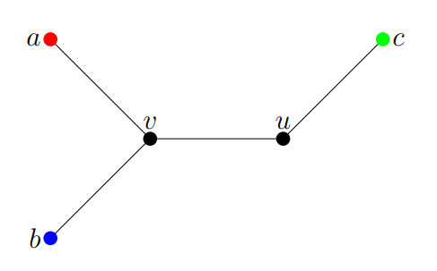
In Example 7.2 below consider the even profile \(\pi = (a,b,u,c)\). The intervals \(I(a,b)\) and \(I(u,c)\) do not intersect. But, if we rearrange \(\pi\) into \(\rho = (a,u,b,c)\), we get the associated intervals \(I(a,u)\) and \(I(b,c)\) intersecting in \(\{v,u\}\), which is precisely \(Med(\pi)\).
In [13] it was proved that the cube-free median graphs satisfy (IIP), of which trees are a prime example. Besides these cube-free median graphs, also the complete bipartite graphs \(K_{2,n}\) satisfy (IIP). In [10] it was shown that, if each block (i.e. maximal 2-connected subgraph) satisfies (IIP), then the whole graph satisfies (IIP).
Now let \(\pi\) be an even profile of length \(2m\) that allows a reordering \(\rho = (y_1, y_2, \ \ldots \ , y_{2m})\) such that \(\bigcap_{i = 1}^m I(y_{2i-1},y_{2i}) \neq \emptyset.\) Due to Betweenness we have \(Med((y_{2i-1},y_{2i})) = I(y_{2i-1},y_{2i})\), for \(i = 1, 2, \ldots , m\). Due to Consistency we have \(Med(\rho) = \bigcap_{i = 1}^m I(y_{2i-1},y_{2i})\). Finally, due to Anonymity we have \(Med(\pi) = Med(\rho)\). In a tree an interval between \(y_{2i-1}\) and \(y_{2i}\) induces the unique path \(P_i\) between \(y_{2i-1}\) and \(y_{2i}\). So \(\rho\) gives us \(m\) paths \(P_1, P_2, \ldots , P_m\) that pairwise have distinct entries of \(\pi\) as end points. Moreover the intersection of these paths is just the path induced by \(Med(\pi)\). Let \((z_1, z_2, \ldots , z_{2m})\) be any reordering of \(\pi\) with \(\bigcap_{i = 1}^m I(z_{2i-1},z_{2i}) \neq \emptyset\). Then, by (A), (B), and (C), also \(\bigcap_{i = 1}^m I(z_{2i-1},z_{2i}) = Med(\pi)\). This is an observation that we will use in the sequel without mention.
Next we consider odd profiles. Let \(\pi = (x_1, x_2, \ldots , x_k)\) be an odd profile on a tree \(T\). Note that \(Med(\pi)\) consists of a single vertex. By \(\pi – x_i\) we denote the profile obtained from \(\pi\) by deleting the entry \(x_i\). We call such a subprofile an entry-deleted profile. Note that it has length \(k-1\), which is even. A consequence of Theorem 7 in [13] on median graphs is the following theorem on trees.
Theorem A. Let \(T\) be a tree, and let \(\pi = (x_1, x_2, \ldots , x_k)\) be an odd profile on \(T\), with \(k > 1\). Then \[Med(\pi) = \bigcap_{i = 1}^{i = k} Med(\pi – x_i).\]
If \(Med(\pi) = \{v\}\), then this implies that \(v \in Med(\pi – x_i)\), for any \(i\). Example 7.2 below shows that \(Med(\pi – x_i)\) might contain more than \(Med(\pi)\).
When \(T\) is a tree with an odd number of vertices, then \(Med(T) = \{x\}\), for some vertex \(x\). Consider the single occurrence profile \(\sigma\) with entries the vertices in \(V – x\), which is an even profile. Due to (IIP) there is a reordering \((y_1, y_2, \ \ldots \ , y_{2m})\) of \(\sigma\) such that \(Med(\sigma) = \bigcap_{I = 1}^m I(y_{2i-1},y_{2i}).\) As observed above, \(Med(\sigma)\) induces the path that is the intersection of the paths induced by these intervals. By Theorem A, we have \(x \in Med(\sigma)\). So we have \(m\) paths, of which the end points are pairwise distinct, that all contain \(x\) as an internal vertex, again a crucial property in the sequel.
We are now ready to study our next centrality.
Mitchell [15] introduced the telephone center of a tree in a slightly informal manner, which served the purpose perfectly. But to generalize the concept to the functional case, we need a more extended model, and a more formal definition.
Let \(T = (V,E)\) be a tree. As usual a vertex of \(T\) is a location, and, in our model for Mitchell’s telephone center, at each location there is located exactly one user. Let \(v\) be a vertex of \(T\). Both the location \(v\), and the user at \(v\) can be represented by the vertex \(v\). A user \(u\) can make a call to another user \(v\). This call will be represented by the path in \(T\) between \(u\) and \(v\). Any internal vertex on this path could serve as a switchboard to facilitate the call. For the younger people amongst us, if you want to know what a switchboard is, just look it up in an old dictionary. These are available at second hand bookstores. Mitchell’s Problem is to find vertices that can serve as a switchboard that facilitates as many simultaneous calls as possible. Mathematically we can formulate this as follows.
Definition 7.1. Two paths in a tree \(T\) are distinct if all four end points of the two paths are distinct.
In this sense two distinct paths both must have positive length. In Example 7.2 the two paths \(P_1 = a,v,u,c\) and \(P_2 = b,v,u\) are distinct in the sense of Definition 7.1, but the paths \(P_1\) and \(Q = a,v,b\) are not.
Example 7.2. Let \(T\) be the tree shown in Figure 1. Then \(Med(T) = \{v\}\).
Note that Mitchell’s Problem was formulated in 1977, when there were only old-fashioned landlines. A vertex can make a call to another vertex. We assume that, at any given time, a vertex can be involved in at most one call, as was the case in 1977. This means that simultaneous calls at any given time are pairwise distinct paths.
Definition 7.3. The switchboard number \(sb^*(v)\) of a vertex \(v\) is the maximum number of pairwise distinct paths that all contain \(v\) as an internal vertex.
The goal is now to find the vertices that maximize this switchboard number. Consider the tree in Example 7.2. Since there are 5 vertices there are at most two distinct paths. The two paths \(P_1 = a,v,u,c\) and \(P_2 = b,v,u\) both contain \(v\) as internal vertex. So \(sb^*(v) = 2\). There are no two distinct paths that both contain \(u\) as an internal vertex, so \(sb^*(u) = 1\). Finally, \(a\), \(b\), and \(c\) are not an internal vertex of any path, so \(sb^*(a) = sb^*(b) = sb^*(c) = 0\). Hence \(v\) is the unique vertex that maximizes the switchboard number, which happens also to be the unique median vertex of \(T\).
Definition 7.4. The telephone center \(Tel(T)\) of a tree \(T = (V,E)\) is the set of vertices \(v\) that maximize the switchboard number \(sb^*(v)\).
In her Note [15] Mitchell gave a straightforward proof that the telephone center of a tree is precisely the centroid of the tree, and hence it is also the median of the tree.
Throughout we now set \(n\) as the number of vertices of \(T\). Letting
\[\ell = \left\lfloor \frac{1}{2} (n-1) \right\rfloor, \tag{3}\] we have \(n = 2\ell +1\) in case \(n\) is odd, and \(n = 2\ell + 2\) in case \(n\) is even. Let \(v\) be a vertex of \(T\). Then we can find \(\ell\) non-intersecting pairs of vertices in \(V – v\), but not more. Each such pair can be taken as the end points of a path in \(T\). Thus we get \(\ell\) pairwise distinct paths, none of which has \(v\) as an end point. Hence \(sb^*(v) \leq \ell\). To prove Mitchell’s Theorem it suffices to show that \(sb^*(v) = \ell\) if and only if \(v\) is in the centroid (or the median) of \(T\), see [15]. Our deliberations involving (IIP) in the last few paragraphs of the previous section also provide us with the tools for a proof of Mitchell’s theorem. We apply (IIP) on the full profile \(\phi\), in case \(n\) is even, and on the single occurrence profile \(\sigma\) with \(\{\sigma\} = V – x\), in case \(n\) is odd and \(x\) is the median vertex. Mitchell’s Theorem will also follow from our results on the functional extensions of the telephone center below.
As noted before, the classical centralities are all with respect to the whole vertex set of the graph, while in the functional extension we seek central vertices with respect to a profile. Then the classical central vertices should be those with respect to a full profile, where each vertex occurs exactly once. In the case of the centroid, see Section 4, the security center, see Section 5, as well as the median, the eccentricity center, and the weight balance center, the functional extension is straightforward, see e.g. [13, 14, 12]. Also, in all these cases the classical central vertices are the output for a full profile.
It turns out that a functional extension of Mitchell’s telephone center is less straightforward. First we take the obvious route, where we extend Mitchell’s model by following it to the letter, see Section 8.1. The consensus function we thus obtain has some peculiar and unexpected properties. Also there does not seem to be a relationship with the median function, even on a path. A characterization of this function still eludes us.
Next we take a different route. We select properties of Mitchell’s model that we consider to be the essential properties, and relax one or two less essential properties in a way that appeals more to the intuition. Thus we obtain three functional extensions that in our view capture the spirit of Mitchell’s model better than the above one, see Sections 8.2, 8.3, and 8.4. Each of these extensions has its own appeal. And each has a close relationship with the median function in its own way.
Recall that, when we extend the case to profiles, the vertices are still locations, but now the entries of the profile are the users. Moreover at a given location there may be no user, or exactly one user, or more than one user. In the case of the telephone center a call is to be made by two users, hence by two profile entries. The call is represented by the path between these two entries, so that the end points of the path are distinct entries of the profile, but not necessarily distinct vertices. Consider for instance the simple profile \(\pi = (x_1, x_2) = (u,u)\) with two distinct entries \(x_1\) and \(x_2\), which are both located at the same vertex \(u\). A call between the two distinct users \(x_1\) and \(x_2\) is represented by the path \(P\) with the distinct entries \(x_1\) and \(x_2\) as end points. Then \(P = u\) is just the path of length 0 with the same vertex \(u\) as begin and end point. We allow \(P\) to be a path representing a call between the two entries of \(\pi\). Following Mitchell, simultaneous calls are to be made by distinct entries. This gives rise to the following definition.
Definition 8.1. Let \(T\) be a tree, and let \(\pi\) be a profile on \(T\). Two paths are \(\pi\)-distinct if all four end points of the two paths are distinct entries of \(\pi\).
The appropriate analogue of the switchboard number as defined in the previous section is as follows.
Definition 8.2.Let \(\pi\) be a profile on a tree \(T\), and let \(u\) be a vertex of \(T\). The classical switchboard number \(sb^*_\pi(u)\) of \(u\) with respect to \(\pi\) is the maximum number of pairwise \(\pi\)-distinct paths that all contain \(u\) as an internal vertex.
Obviously, the path \(P\) between two entries \(x_1\) and \(x_2\) with \(x_1 = x_2 = u\) is excluded in any count for this switchboard number, because \(P\) has no internal vertices.
We define a location function using the switchboard number \(sb^*(v)\) from Definition 8.2. Although this location function clearly fits strictly into the original model of Mitchell, we will see that it has some problematic aspects. Therefore we have chosen not to call it \(Tel\), but instead to use Greek letters, in the hope that it is not all Greek to the reader. Thus we define the location function \(\tau \epsilon \lambda : V^* \rightarrow \mathcal{P}_{ne}(V)\) by \[\tau \epsilon \lambda(\pi) = \{ x \mid x \text{ maximizes } sb^*_\pi(x) \}.\]
As observed, the definition of \(\tau\epsilon\lambda\) fits strictly into the original model of Mitchell. Also the output \(\tau \epsilon \lambda(\phi)\) of a full profile \(\phi\) is the classical telephone center \(Tel(T)\) sensu Mitchell. So \(\tau\epsilon\lambda\) is a proper functional extension. This gives rise to the following problem.
Problem 8.3. Let \(T = (V,E)\) be a tree. What are the properties of a telephone center function \(\tau \epsilon \lambda : V^* \rightarrow \mathcal{P}_{ne}(V)\) such that, in determining a switchboard number of vertex \(u\), only paths that are pairwise \(\pi\)-distinct and contain \(u\) as an internal vertex are counted?
Let us consider some examples to see what can happen in this case. We take a few profiles of length 4 on the path of length 5, see Figure 2.

First consider the profile \(\pi = (b,c,d,e)\). Clearly we have \(Med(\pi) = \{c,d\}\). There are no two \(\pi\)-distinct paths that share an internal vertex. Moreover, \(c\) and \(d\) are the only vertices that are an internal vertex of a path between entries of \(\pi\), so \(\tau \epsilon \lambda(\pi) = \{c,d\} = Med(\pi)\). Next consider the profile \(\rho = (a,c,d,f)\). Now we have \(Med(\rho) = \{c,d\} \subsetneqq \{b,c,d,e\} = \tau \epsilon \lambda(\rho)\). Then consider the profile \(\sigma = (a,a,c,c)\). Then \(\tau \epsilon \lambda(\sigma) = \{b\} \subsetneqq \{a,b,c\} = Med(\sigma)\). Finally consider the profile \(\delta = \{a,d,d,d\}\). Then \(Med(\delta) = \{d\}\), whereas \(\tau\epsilon\lambda(\delta) = \{b,c\}\), and we have \(\tau\epsilon\lambda(\delta) \cap Med(\delta) = \emptyset\). These examples show that there is not a clear-cut relation between the functions \(\tau\epsilon\lambda\) and \(Med\) on a tree, even on a path. Also it suggests that Problem 8.3 might not be an easy problem. But there is an additional problem. Let \(\pi\) be a profile on a tree \(T\) with \(\{\pi\}\) being a single vertex or two adjacent vertices. Then no path between entries of \(\pi\) has internal vertices. So each vertex \(v\) has switchboard number \(sb^*(v) = 0\). Hence the output for such profiles is the whole vertex set \(V\). So a switchboard might be located far away from the set of users who make the calls, and has no relation with paths between entries. This is counter-intuitive. We leave Problem 8.3 as an open problem.
In the definition of the location function \(\tau\epsilon\lambda\) we followed Mitchell’s original model to the letter. Note that \(x\) being an internal vertex of a path \(P\) between the vertices \(u\) and \(v\) implies that \(x\) is between \(u\) and \(v\), that is, lies in \(I(u,v)\). But with profiles, we saw that the requirement that a switchboard should be located at an internal vertex of paths representing calls, also had the consequence that a switchboard might not even be between any two callers. What if we don’t follow the model to the letter but instead focus on the spirit of the model? That is, we give priority to the switchboard always being located between callers instead of it being always located at an internal vertex. The latter requirement created the possibility that it is not between some pairs of callers. In the sequel our point of departure is the following set of requirements.
Let \(\pi = (x_1, x_2,\ldots , x_k)\) be a profile on the tree \(T\).
\(1.\) A call is made by two distinct entries \(x_i\) and \(x_j\) of \(\pi\). It is represented by the path between \(u = x_i\) and \(v = x_j\).
\(2.\) Two simultaneous calls are represented by \(\pi\)-distinct paths, of which the four end points are distinct entries of \(\pi\).
\(3.\) A switchboard that facilitates a call between distinct entries \(x_i\) and \(x_j\) should be ’between’ \(u = x_i\) and \(v = x_j\), that is, it should be on the path between \(u\) and \(v\).
Now for a profile \(\pi\), we search for vertices \(x\) that maximize the number of pairwise \(\pi\)-distinct paths such that \(x\) is on each of these paths.
Consider again the above profile \(\delta = (x_1, x_2, x_3, x_4) = (a,d,d,d)\) in Figure 2. There are four distinct users. User \(x_1\) is located at vertex \(a\), the other three are located at \(d\). In search of a telephone center for \(\delta\), we consider the possible calls between profile entries. Since there are four entries, there can be two simultaneous calls. Say there is a call between \(x_1\) and \(x_2\), represented by the path \(P_1\) between the vertices \(a\) and \(d\). And there is a call between \(x_3\) and \(x_4\), represented by the path between \(x_3\) and \(x_4\), which is the path \(P_2 = d\). Note that the begin point and end point of \(P_2\) are the same vertex \(d\), but as entries of \(\delta\) they are distinct. Back in 1977 such a call might have seemed science fiction, but nowadays this is perfectly possible where all users have their own cell phone (how it will be 49 years from now is still a mystery). Note that any other way of pairing the entries to make simultaneous calls results in the same two paths \(P_1\) and \(P_2\). The only vertex that is on two \(\delta\)-distinct paths is \(d\). The vertices \(a,b,c\) are each only on \(P_1\), whereas the other two vertices \(e,f\) are neither on \(P_1\) nor on \(P_2\). So vertex \(d\) is the candidate for the location of the switchboard.
These deliberations give rise to the following alternative definition of the switchboard number.
Definition 8.4. Let \(\pi\) be a profile on a tree \(T\), and let \(u\) be a vertex of \(T\). The switchboard number \(sb_\pi(u)\) of \(u\) with respect to \(\pi\) is the maximum number of pairwise \(\pi\)-distinct paths that all contain \(u\), either as an internal vertex or as an end point.
To compare this with Mitchell’s switchboard number in Definition 7.3 we define \(sb(u) = sb_\phi(u)\), where \(\phi\) is a full profile on \(T\). So \(sb(u)\) is a switchboard number for calls made by the vertices of the tree. In the case of an even tree with \(2\ell +2\) vertices there is a direct relation between Mitchell’s \(sb^*(u)\) and our \(sb(u)\).
Lemma 8.5. Let \(T\) be a tree with \(n = 2\ell + 2\) vertices, and let \(v\) be a vertex of \(T\). Then \(sb(v) = sb^*(v) + 1\).
Proof. Let \(v\) be a vertex of \(T\) with \(sb^*(v) = s\). Let \(P_1, P_2, \ldots , P_s\) be a set of pairwise distinct paths that realizes this maximum number. Any such path \(P_i\) contains \(v\) as internal vertex, and so is of length at least 2. Since \(n\) is even, there is besides \(v\) at least one other vertex \(u\) that is not an end point of any \(P_i\). Let \(P_{s+1}\) be the path between \(u\) and \(v\). Then \(P_1, P_2, \ldots , P_{s+1}\) are \(s+1\) pairwise distinct paths that all contain \(v\). Note that in any set of pairwise distinct paths that contain \(v\) as a vertex, at most one has \(v\) as end point, and all other paths necessarily contain \(v\) as internal vertex. So, if \(sb^*(v) = s\), then the maximum number of pairwise distinct paths that contain \(v\) as either an internal vertex or an end point is \(s+1\). ◻
For odd profiles the situation is different. Let \(\pi = (x_1, x_2, \ldots , x_k)\) be a profile on a tree \(T\). Set \(m = \lfloor \frac{1}{2} k \rfloor\). Clearly there are at most \(m\) pairwise \(\pi\)-distinct paths, so \(sb_\pi(u) \leq m\), for all vertices \(u\) of \(T\). For a vertex \(u\) of \(T\) we define a \(\pi\)-call set for \(u\) to be a set \(\mathtt{Q}_\pi(u)\) of order \(sb_\pi(u)\) of pairwise \(\pi\)-distinct paths that all contain \(u\), that is, a set of paths that realizes \(sb_\pi(u)\). Note that, if \(k = 1\), so that \(m = 0\), then \(\mathtt{Q}_\pi(u) = \emptyset\). For a vertex \(u\) not in \(Med(\pi)\) we can describe such a set \(\mathtt{Q}_\pi(u)\) quite precisely.
Lemma 8.6. Let \(\pi = (x_1, x_2, \ldots , x_k)\) be a profile on a tree \(T\). Let \(u\) be a vertex not in \(Med(\pi)\), and let \(x\) be the neighbor of \(u\) closer to \(Med(\pi)\). Then \(sb_\pi(u) = |\pi_{ux}| < \frac{1}{2} k\), and each path \(Q\) in \(\mathtt{Q}_\pi(u)\) contains both \(u\) and \(x\).
Proof.Since \(u \notin Med(\pi)\), we have \(|\pi_{ux}| < |\pi_{xu}|\), so \(r = |\pi_{ux}| < \frac{1}{2} k\). If \(\pi_{ux}\) is empty, then we cannot find any path between entries that contains \(u\), so \(sb_\pi(u) = 0 = |\pi_{ux}|\), and \(\mathtt{Q}_\pi(u) = \emptyset\). Otherwise we can pair each entry in \(\pi_{ux}\) with a different entry in \(\pi_{xu}\), thus obtaining \(r\) paths that are pairwise \(\pi\)-distinct. These necessarily all contain \(u\) as well as \(x\). Clearly, any path between entries of \(\pi\) that contains \(u\) has one end in \(\pi_{ux}\). So we cannot get more pairwise \(\pi\)-distinct paths that all contain \(u\). Hence \(sb_\pi(u) = r\). Moreover, to get so many paths, we cannot pair two entries of \(\pi_{ux}\). So all paths in \(\mathtt{Q}_\pi(u)\) contain both \(u\) and \(x\). This completes the proof. ◻
There is a distinction between even and odd profiles for which vertices we actually have \(sb_\pi(u) = m\).
Lemma 8.7. Let \(\pi = (x_1, x_2, \ldots , x_{2m})\) be an even profile on a tree \(T\). Then \(v \in Med(\pi)\) if and only \(sb_\pi(v) = m\).
Proof. Due to (IIP) there is a reordering \(\rho = (y_1, y_2, \ \ldots \ , y_{2m})\) of \(\pi\) such that \[Med(\pi) = Med(\rho) = \bigcap_{I = 1}^m I(y_{2i-1},y_{2i}).\] The \(m\) intervals in the intersection clearly induce \(m\) pairwise \(\pi\)-distinct paths, of which the intersection is \(Med(\pi)\). So, for \(v \in Med(\pi)\) we have \(sb_\pi(v) = m\).
Next consider a vertex \(u \notin Med(\pi)\). By Lemma 8.6, there are no \(m\) pairwise \(\pi\)-distinct paths that all contain \(u\), and we are done. ◻
Lemma’s 8.5 and 8.7 provide us with another proof of Mitchell’s original theorem in the case of a tree with an even number of vertices.
Corollary 8.8. Let \(T\) be a tree with an even number of vertices. Then \(Tel(T) = Med(T)\).
Proof. Lemma 8.5 tells us that the telephone center sensu Mitchell consists of the vertices \(u\) that maximize \(sb(u)\). Let \(\phi\) be a full profile on \(T\). Then Lemma 8.7 tells us that \(Tel(T) = Med(\phi)\). Clearly, the median set \(Med(\phi)\) of a full profile is the median \(Med(T)\) of the tree, and we are done. ◻
Now we consider the case of odd profiles. When simultaneous calls are made then there is always an entry that is not involved in a call. We call such an entry a leftover entry. In the case of a tree with \(n = 2\ell + 1\) vertices a leftover entry of a full profile is just a leftover vertex. We will see that the leftovers play a crucial role in the development of our functional extension of the telephone center in the odd case.
A special case are the profiles \(\xi = (x_1)\) of length 1. Then no call is possible, and \(x_1\) is the leftover entry. This is sort of an anomaly, and below we present one or two alternatives for dealing with profiles of length 1. Recall that an entry-deleted profile \(\pi – x_i\) is defined as a subprofile obtained by deleting the entry \(x_i\). Subprofiles may be empty, as is the case for \(\xi – x_1\). We use the convention that \(Med(\emptyset) = V\).
Let \(\pi = (x_1, x_2, \ldots , x_k)\) be an odd profile with \(k = 2m+1 > 1\). Obviously, the maximum number of pairwise \(\pi\)-distinct paths is \(m\). Let \(P_1, P_2, \ldots P_m\) be pairwise \(\pi\)-distinct paths. These paths have \(2m\) different entries as end point, and the leftover entry, say \(x_i\), is not an end point of any of these paths. Hence these paths are also \(m\) pairwise \((\pi – x_i)\)-distinct paths. The median sets of the entry-deleted profiles of \(\pi\) play an essential role in our functional extension of the telephone center. Let \[Z(\pi) = \bigcup_{i = 1}^k Med(\pi – x_i). \label{Xmed} \tag{4}\]
For want of a better term, we call \(Z(\pi)\) the extended median set of the odd profile \(\pi\). If \(\xi = (x_1)\) is a profile of length 1, then, applying the convention above for the empty subprofile on Equality (4), we get \(Z(\xi) = V\).
In Example 1, let \(\phi\) be the full profile \((x_1, x_2, x_3, x_4, x_5) = (a,b,c,u,v)\). Then we have \(Med(\phi – a) = Med(\phi – b) = Med(\phi – v) = \{v,u\}\), and \(Med(\phi – u)\) \(= Med(\phi – c) = \{v\}\). So \(Z(\phi) = \{v,u\}\), and \(Med(\phi) = \{v\} = \bigcap_{i = 1}^5 Med(\phi – x_i)\), in accordance with Theorem A.
Lemma 8.9. Let \(\pi = (x_1, x_2, \ldots , x_{2m+1})\) be an odd profile on a tree \(T\). Then the extended median set \(Z(\pi)\) of \(\pi\) consists precisely of the vertices \(z\) in \(T\) for which there are \(m\) pairwise \(\pi\)-distinct paths all containing \(z\).
Proof. First let \(m = 0\), so that \(\pi\) is of length 1. Then there is no path between distinct entries of \(\pi\). Hence \(Z(\pi) = V = Med(\emptyset)\).
Next let \(m > 0\). Take a vertex \(z \in Z(\pi)\). Then \(z\) lies in a median set \(Med(\pi – x_i)\), for some entry \(x_i\) of \(\pi\). The entry-deleted profile \(\pi – x_i\) is an even profile, so by (IIP) there are \(m\) pairwise \((\pi – x_i)\)-distinct paths such that their intersection is precisely \(Med(\pi – x_i)\). Clearly, these \(m\) pairwise \((\pi – x_i)\)-distinct paths are also pairwise \(\pi\)-distinct. They all contain \(z\).
Conversely, let \(w\) be a vertex not in \(Z(\pi)\). Then \(w\) is not in \(Med(\pi – x_i)\), for all \(i = 1, 2, \ldots , k\). Consider such an entry-deleted profile \(\pi – x_i\). It is of length \(2m\). We apply Lemma 8.6 on this profile. The number of pairwise \((\pi – x_i)\)-distinct paths, all containing \(z\), is strictly less than \(\frac{1}{2}(k-1) = m\). This holds for all \(i = 1, 2, \ldots , k\). So the maximum number of pairwise \(\pi\)-distinct paths that contain \(w\) is strictly less than \(m\). ◻
Lemma 8.9 provides us with a well-defined location function \(Phon\) that captures important aspects of Mitchell’s telephone center. We define the location function \(Phon : V^* \rightarrow \mathcal{P}_{ne}(V)\) by \[Phon(\pi) = \{ x \mid x \text{ maximizes } sb_\pi(x) \}.\]
Theorem 8.10. Let \(T\) be a tree, and let \(\pi = (x_1, x_2, \ldots , x_k)\) be a profile on \(T\). Then \[Phon(\pi) = \begin{cases} Med(\pi) &\text{ if } \pi \text{ is even},\\ \bigcup_{i = 1}^k Med(\pi – x_i) &\text{ if } \pi \text{ is odd}. \end{cases}\]
Proof. By Lemma 8.7, we have \(Phon(\pi) = Med (\pi)\) for even profiles. And by Lemma 8.9, we have \(Phon(\pi) = Z(\pi) = \bigcup_{i = 1}^k Med(\pi – x_i)\), for odd profiles. ◻
The location function \(Phon\) is not a functional extension of the telephone center in the proper sense. For a full profile \(\phi\) we have \(Tel(T) \subseteq Phon(\phi)\). But for trees with an odd number of vertices we may have \(Tel(T) \neq Phon(\phi)\). So it is not a ‘perfect’ functional extension of the classical telephone center, although it captures basic intuitive features of the classical case.
In the next Subsections we present two possible location functions that are a more ‘perfect’ functional extension. We conclude this section with an exploration of what form the set \(Z(\pi)\) can take. First we have a look at Example 7.2 again. Consider the profile \(\pi = (a,b,c)\) of length 3. Then \(Med(\pi – a)\) induces the path between \(b\) and \(c\), and \(Med(\pi – b)\) induces the path between \(a\) and \(c\), and finally \(Med(\pi – c)\) induces the path between \(a\) and \(b\). So \(Z(\pi)\) induces the whole tree, which is a subdivision of the star \(K_{1,3}\). Recall that a subdivision is obtained by (repeatedly) “inserting” a vertex on an edge. We call such a subdivision an aster, cf. [8]. It is a tree with a unique vertex of degree 3, whereas all other vertices have degree less than 3. Besides the usual median sets of profiles in trees, that is, a single vertex or a path, the aster is the only other possibility for \(Z(\pi)\), as we will see in Proposition 8.11.
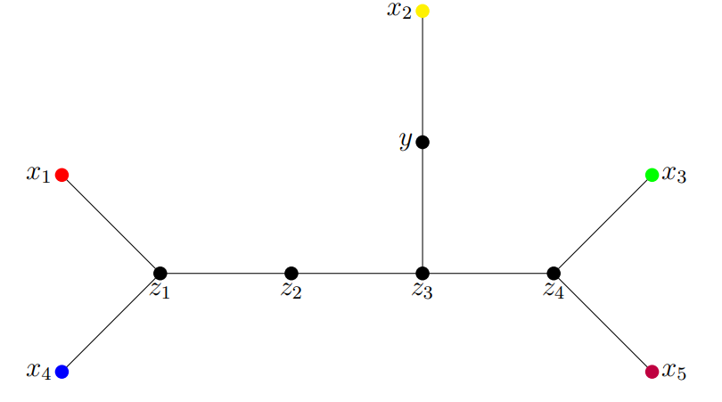
We use Figure 3 as illustration for the proof of Proposition 8.11. We want to draw attention to the position of the vertices \(x_1, x_2, x_3, x_4, x_5\) with respect to some specific paths. Clearly \(x_2\) lies to the north of the path \(P = z_1, z_2, z_3, z_4\), whereas \(x_1\) and \(x_4\) lie to the west and \(x_3\) and \(x_5\) lie to the east of \(P\). Take the path \(P_1 = z_1, z_2, z_3\). Then \(x_1\) and \(x_4\) still lie to the west of \(P_1\), whereas now \(x_2\), \(x_3\), and \(x_5\) lie to the east of \(P_1\). For the path \(P_2 = z_3, z_4\), the vertices \(x_1\), \(x_2\), and \(x_4\) lie to the west of \(P_2\), whereas \(x_3\) and \(x_5\) lie to the east of \(P_2\).
Recall that a vertex can be viewed as a path of length 0. This is used in the formulation of the next Proposition.
Proposition 8.11. Let \(T\) be a tree, and let \(\pi = (x_1, x_2, \ldots , x_k)\) be an odd profile on \(T\) of length \(k > 1\). Then either \(Z(\pi)\) induces a path, or \(Z(\pi)\) induces an aster, in which case \(\pi\) is of length 3 and consists of three entries that are the leaves of the aster.
Proof. Set \(k = 2m+1\), and let \(Med(\pi) = \{v\}\). Note that we have \(m \geq 1\). For each entry \(x_i\), the subprofile \(\pi – x_i\) is an even profile, and the median set \(Med(\pi – x_i)\) consists of the single vertex \(v\) or a of a path of positive length that contains \(v\).
Let \(m = 1\), so that \(\pi = (x_1, x_2, x_3)\) is a profile of length 3. We consider two cases.
First let \(x_1, x_2, x_3\) be located at vertices on a path. This includes the case that two or three entries are located at the same vertex. Now \(\pi – x_i\) is a profile of length 2, so \(Med(\pi – x_i)\) induces a path, possibly of length 0, between the two entries in \(\pi – x_i\). Due to anonymity, we may assume that \(x_2\) lies between \(x_1\) and \(x_3\). Then \(Med(\pi – x_2)\) induces the path \(P\) between \(x_1\) and \(x_3\), and \(x_2\) is on this path. Now \(Med(\pi – x_1)\) induces the subpath of \(P\) between \(x_2\) and \(x_3\), and \(Med(\pi – x_3)\) induces the subpath of \(P\) between \(x_2\) and \(x_1\). Hence \(Z(\pi) = Med(\pi – x_2)\) induces the path \(P\), which might be of length 0.
The second case is that \(x_1, x_2, x_3\) are not located on one path. This means that they are located at three vertices \(u,v,w\), respectively, that are the leaves of the aster consisting of the three paths between \(u\), \(v\), and \(w\). Now \(Med(\pi – x_1)\) induces the path between \(v\) and \(w\), and \(Med(\pi – x_2)\) induces the path between \(u\) and \(w\), and finally \(Med(\pi – x_3)\) induces the path between \(u\) and \(v\). Hence \(Z(\pi)\) induces this aster with leaves \(x_1 = u\), \(x_2 = v\), and \(x_3 = w\). This completes the proof of the case \(m = 1\).
Next let \(m > 1\). If \(Med(\pi – x_i)\) is the single vertex \(v\), for all \(i = 1, 2, \ldots , k\), then \(Z(\pi) = \{v\}\), and we are done. So assume that there is an entry-deleted subprofile, for which the median set induces a path of positive length. We choose entry \(x_i\) such that the path induced by \(Med(\pi – x_i)\) is as long as possible. Let \(P = z_1, z_2, \ldots , z_s\) be this path. Note that \(s > 1\). Let \(\pi_{west}\) be the subprofile of \(\pi – x_i\) to the west of \(P\), and let \(\pi_{east}\) be the subprofile of \(\pi – x_i\) to the east of \(P\). Then we have \(|\pi_{west}| = |\pi_{east}| = m\). The maximality of \(P\) implies the following. Let \(z_{s+1}\) be any neighbor of \(z_s\) not on \(P\). So \(z_{s+1}\) lies to the east of \(P\). Let \(P^\prime = P,z_{s+1}\) be the path obtained by extending \(P\) to the east by adding \(z_{s+1}\). Because of the maximality of \(P\) there are less than \(m\) entries of \(\pi\) to the east of \(P^\prime\), and some entries of \(\pi_{east}\) will lie to the north of \(P^\prime\). Similarly, \(P\) cannot be extended to the west. We use this in the sequel.
We consider a couple of cases depending on where \(x_i\) is located with respect to \(P\).
First let \(x_i\) be nor to the west neither to the east of \(P\). Then either \(x_i\) is an internal vertex of \(P\), say, \(x_i = z_t\), or \(x_i\) lies to the north of \(P\), and let \(z_t\) be the vertex on \(P\) closest to \(x_i\). Clearly we have \(1 < t < s\). In Figure 3, we would have \(x_i = x_2\) and \(z_t = z_3\). Let \(P_1\) be the path \(z_1, z_2, \ldots , z_t\), and let \(P_2\) be the path \(z_t, z_{t+1}, \ldots , z_s\). The union of these two paths constitute \(P\). Now \(\pi_{west}\) lies to the west of \(P_1\) as well as \(P_2\), and \(\pi_{east}\) lies to the east of \(P_1\) as well as \(P_2\). Entry \(x_i\) lies to the east of \(P_1\), but to the west of \(P_2\). Take any entry \(x_j\) of \(\pi\) distinct from \(x_i\). Then \(x_j\) lies to the west or to the east of \(P\), see Fig. 3. First let \(x_j\) be to the west of \(P\). Then exactly half of \(\pi – x_j\) lies to the west of \(P_2\), and exactly half of \(\pi – x_j\) lies to the east of \(P_2\). If we extend \(P_2\) either to the east or the west, some entries will lie either on or to the north of the extended path, and the rest of \(\pi – x_j\) is not equally distributed over west and east anymore. Therefore \(Med(\pi – x_j)\) induces the path \(P_2\). Similarly, if \(x_j\) lies to to the east of \(P\), then it follows that \(Med(\pi – x_j)\) induces the path \(P_1\). Hence \(Z(\pi)\) induces the path \(P\).
Second, let \(x_i\) lie to the west of \(P\). Then there are \(m+1\) entries of \(\pi\) to the west and \(m\) entries to the east of \(P\). For each \(x_j\) to the west of \(P\), exactly half of \(\pi – x_j\) lies to the west of \(P\) and exactly half lies to the east of \(P\). So \(P\) is included in the path induced by \(Med(\pi – x_j)\). Since \(P\) is the longest such path, \(Med(\pi – x_j)\) induces \(P\), for all \(x_j\) to the west of \(P\).
Now let \(x_j\) be an entry to the east of \(P\). Consider the subprofile \(\pi – x_j\). Then \(m-1\) entries of \(\pi – x_j\) lie to the east of the edge \(f = z_1z_2\) on \(P\), and \(m+1\) entries lie to the west of this edge. So \(Med(\pi – x_j)\) is located in \(V_{z_1z_2}\). Since the median vertex \(v\) of \(\pi\) is in the median set of all entry-deleted profiles, and thus lies on \(P\), it follows that \(v = z_1\). Now assume that \(Med(\pi – x_j)\) consists of more vertices than just \(v\). Then there is a neighbor \(x\) of \(v\) in \(Med(\pi – x_j)\). Clearly, \(x\) lies in \(V_{z_1z_2} = V_{vz_2}\). With respect to the edge \(xv\), we must have that half of \(\pi – x_j\) lies in \(V_{xv}\) and half of \(\pi – x_j\) lies in \(V_{vx}\). All of the \(m-1\) entries in \(\pi_{east} – x_j\) lie in \(V_{vx}\). So there is exactly one entry \(x_r\) of \(\pi_{west}\) that lies in \(V_{vx}\), whereas the other \(m\) entries of \(\pi_{west}\) lie in \(V_{xv}\). Consider the entry-deleted profile \(\pi – x_r\). Half of its entries lies in \(\pi_{east}\) and the other half lies in \(V_{xv}\). So \(Med(\pi – x_r)\) contains all vertices of the path \(P\) plus also \(x\). Hence it induces a path that is longer than \(P\). This contradicts the maximality of \(P\). So we conclude that \(Med(\pi – x_j) = \{v\}\). This holds for every choice of \(x_j\) in \(\pi_{east}\). Again we have shown that \(Z(\pi)\) induces the path \(P\).
The case that \(x_i\) lies to the east of \(P\) follows in the same way as the previous case with interchanging the roles of west and east. This concludes our final case. ◻
Let \(\pi = (x_1, x_2, \ldots x_{2m+1})\) be an odd profile on a tree \(T\) with \(m > 1\), and let \(Med(\pi) = \{v\}\). Theorem A tells us that \(v\) lies in \(Med(\pi – x_i)\), for each entry \(x_i\) of \(\pi\). Hence there exist \(m\) pairwise \((\pi – x_i)\)-distinct paths all containing \(v\), for each \(i\). There is a notable distinction between \(v\) and any vertex \(z\) in \(Z(\pi)\) distinct from \(v\). Let us have a look again at Example 7.2. Let \(\phi\) be a full profile on \(T\). We considered the paths \(P_1 = a,v,u,c\) and \(P_2 = b,v,u\), which have \(v\) as well as \(u\) in common. Their intersection constitutes the median set of the entry-deleted profile \(\phi – v\), that is, \(Med(\phi – v) = \{u,v\}\). Now conisder the entry-deleted profile \(\phi – u\). Any two \((\phi – u)\)-distinct paths \(Q_1\) and \(Q_2\) share \(v\) but no other vertex. It is simple to check that any other two \(\phi\)-distinct paths that intersect both contain \(v\). On the other hand there are \(\phi\)-distinct paths that both contain \(u\), but there are also \(\phi\)-distinct paths that intersect, where only one of the two contains \(u\). So this distinguishes \(v\) and \(u\). For the general case this phenomenon is established in the next Lemma.
Lemma 8.12. Let \(\pi = (x_1, x_2, \ldots x_{2m+1})\) be an odd profile on a tree \(T\) with \(m > 0\), and let \(v\) be the median vertex of \(\pi\). Then, for any vertex \(z \in Z(\pi) – \{v\}\), there exists an entry \(x_j\) in \(\pi\) such that there are no \(m\) pairwise \((\pi – x_j)\)-distinct paths all containing \(z\).
Proof. By Theorem A, \(\{v\} = Med(\pi) = \bigcap_{i = 1}^k Med(\pi – x_i)\). Take \(z \in Z(\pi) – \{v\}\). Then there exists an entry \(x_j\) such that \(z \notin Med(\pi – x_j)\). Now \(\pi – x_j\) is an even profile of length \(2m\). So by (IIP), any \(m\) pairwise \((\pi – x_j)\)-distinct paths that have a nonempty intersection have \(Med(\pi – x_j)\) as intersection. This intersection does not contain \(z\). Hence there are no \(m\) pairwise \((\pi – x_j)\)-distinct paths that all contain \(z\). ◻
This lemma provides us with a tool to distinguish between the unique median vertex \(v\) of the odd profile \(\pi\) and any other vertex of the tree.
First let \(\pi = (x_1, x_2, \ldots , x_k)\) be a profile with \(k > 1\), and set \(m = \lfloor \frac{1}{2} k \rfloor\). Then \(k = 2m\) or \(2m+1\). Note that \(m > 0\). The maximum number of pairwise \(\pi\)-distinct paths is \(m\). Moreover, by (IIP), we know that there exist \(m\) pairwise \(\pi\)-distinct paths that have a nonempty intersection. Recall that a \(\pi\)–call set \(\mathtt{Q}_\pi(u)\) is a set of order \(sb_\pi(u)\) of pairwise \(\pi\)-distinct paths that all contain \(u\). Clearly, the order of a \(\pi\)-call set is at most \(m\). A maximum \(\pi\)-call set is a \(\pi\)-call set of order \(m\).
Next observe that, if \(\xi = (x_1)\) is a profile of length 1, then there exists no path between distinct entries of \(\xi\). Hence there is no \(\xi\)-call set for any vertex in \(T\).
For any profile \(\pi\) on \(T\), we define \[Tel(\pi) = \{x \mid x \mbox{ lies in each maximum } \pi \mbox{-call set } \}.\] This defines a location function \(Tel : V^* \rightarrow \mathcal{P}_{ne}(V)\). Note that, by default, we have \(Tel(\xi) = V\), for any profile \(\xi\) of length 1. By Lemma’s 8.7 and 8.12, we get the following theorem.
Theorem 8.13. Let \(T\) be a tree, and let \(\pi = (x_1, x_2, \ldots , x_k)\) be a profile on \(T\). Then \[Tel(\pi) = \begin{cases} \ \ V &\text{ if } \ k = 1,\\ Med(\pi) &\text{ if } \ k > 1. \end{cases}\]
Note that, for a full profile \(\phi\), we have \(Tel(\phi) = Med(\phi) = Med(T) = Tel(T)\). Hence \(Tel\) also catches this aspect of Mitchell’s telephone center. On the other hand, it is not solely defined by the value of the switchboard number. We had to add the special condition on maximum \(\pi\)-call sets. So the switchboard number does not work as one would desire form the perspective of Mitchell’s model. Moreover, for profiles \(\xi\) of length 1, we have \(Tel(\xi) = V\), so \(Tel(\xi) \neq Med(\xi)\). In the next section we present a location function that is sort of intermediate between \(Phon\) and \(Tel\), and is defined solely by a switchboard number. Moreover, for profiles of length 1 the output will be the median set.
We return to the idea of leftover entry. Let \(\pi = (x_1, x_2, \ldots , x_k)\) be an odd profile with \(k = 2m + 1\), and let \(v\) be the median vertex of \(\pi\). For any \(\pi\)-call set \(\mathtt{Q}_\pi(v) = \{P_1, P_2, \ldots , P_m\}\), there is exactly one entry that is not an end point of any of the paths \(P_i\). This entry \(x_j\) is the leftover entry. Now we define the path \(P_{m+1}\) to be the path with begin and end point entry \(x_j\). This does not represent a call between two distinct users, but we can interpret it as: entry \(x_j\) is making a selfie at the same time as the calls \(P_1, P_2, \ldots , P_m\) are made. If \(x_j\) is an entry located at \(v\), then we can add \(P_{m+1}\) to \(\mathtt{Q}_\pi(v)\) to obtain a set of \(m + 1\) paths that all contain \(v\). We call this an extended \(\pi\)-call set for \(v\). We will use this idea below to define an alternative switchboard number that allows a selfie to be added to a \(\pi\)-call set. If \(x_j\) is an entry located at a vertex \(u\) distinct from \(v\), then adding the selfie \(P_{m+1}\) to \(P_1, P_2, \ldots , P_m\) would result in a set of paths that does not have \(v\) in its intersection. In this case the extended set of paths is of no use for determining a switchboard number of \(v\).
Let \(\pi = (x_1, x_2, \ldots , x_k)\) be a profile on a tree \(T\), and set \(m = \lfloor \frac{1}{2} k \rfloor\). Let \(u\) be a vertex of \(T\), and consider a \(\pi\)-call set \(\mathtt{Q}_\pi(u) = \{P_1, P_2, \ldots , P_s\}\) for \(u\). Assume that \(2s < k\), so that there are leftover entries. Let \(x_j\) be a leftover entry located at a vertex \(w\), and consider the selfie \(P_{s+1} = w\). In the case that \(w = u\), we can add \(P_{s+1}\) to \(\mathtt{Q}_\pi(u)\) to create an extended \(\pi\)-call set \(\mathtt{Q}^\prime_\pi(u) = \{P_1, P_2, \ldots , P_s, P_{s+1}\}\) that has \(u\) in its intersection. Otherwise the paths \(P_1, P_2, \ldots , P_{s+1}\) do not have \(u\) in its intersection, and the \(\pi\)-call set of \(u\) cannot be extended. In the next Lemma we determine for which cases an extended \(\pi\)-call set is possible.
Lemma 8.14. Let \(T\) be a tree, let \(u\) be a vertex of \(T\), and let \(\pi = (x_1, x_2, \ldots , x_k)\) be a profile on \(T\) with \(m = \lfloor \frac{1}{2} k \rfloor\). Then there exists an extended \(\pi\)-call set for \(u\) if and only if \(k = 2m+1\), \(Med(\pi) = \{u\}\), and there is an entry of \(\pi\) at \(u\).
Proof. First let \(\pi\) be an odd profile of length \(k = 2m + 1\), let \(Med(\pi) = \{v\}\), and let \(x_i\) be an entry of \(\pi\) located at \(v\), so that \(\pi – x_i\) is an even profile of length \(k = 2m\). We have \(v \in Med(\pi – x_i)\). So there are \(m\) pairwise distinct \((\pi – x_i)\)-paths \(P_1, P_2, \ldots , P_m\) all containing \(v\). These paths are also pairwise \(\pi\)-distinct. So they form a \(\pi\)-call set \(\mathtt{Q}_\pi(v)\) The leftover entry for these paths is \(x_i = v\). So we can add the path \(P_{m+1} = v\) to form the extended \(\pi\)-call set \(\mathtt{Q}^\prime_\pi(v) = \{P_1, P_2, \ldots , P_m, P_{m+1}\}\) for \(v\), of which the intersection is precisely \(\{v\}\).
For the converse, let \(P_1, P_2, \ldots , P_s\) be the pairwise \(\pi\)-distinct paths in a \(\pi\)-call set \(\mathtt{Q}_\pi(u)\) for \(u\). The question now is under which conditions can we extend this \(\pi\)-call set. It can only be extended if there are leftover entries, so we must have \(2s < k\). Assume that \(u\) is not a median vertex of \(\pi\), and let \(x\) be the neighbor of \(u\) closer to \(Med(\pi)\). By Lemma 8.6, each \(P_i\) contains the edge \(ux\), and exactly one end point is an entry in \(\pi_{ux}\), whereas the other end point is in \(\pi_{xu}\). Moreover, we have \(|\pi_{ux}| = s\). So each entry in \(\pi_{ux}\) is end point of one of these paths. In particular, if there are entries located at \(u\), then these are such an end point, and thus cannot be a leftover entry. The only way to extend \(\mathtt{Q}_\pi(u)\) would be by a selfie of a leftover entry located at \(u\). So we cannot extend this \(\pi\)-call set.
Next assume that \(u\) is a median vertex of \(\pi\). If \(\pi\) were an even profile, then we would have \(s = m\), and there would be no leftover entry. So \(\pi\) must be odd, that is \(k = 2m+1\), and \(s = m\). But now \(u\) is the unique median vertex of \(\pi\). A leftover entry distinct form \(u\) cannot be added as a selfie to extend \(\mathtt{Q}_\pi(u)\). The only leftover entry that could be used to extend this set would be an entry \(x_j\) located at \(u\). And, as we saw above, in this case we can indeed extend \(\mathtt{Q}_\pi(u)\) to the set \(\mathtt{Q}^\prime_\pi(u)\). ◻
We use these extended \(\pi\)-call sets to define a new switchboard number. To simplify the definition we use the previous switchboard number \(sb_\pi(u)\).
Definition 8.15. Let \(T\) be a tree, and let \(\pi = (x_1, x_2, \ldots , x_k)\) be a profile on \(T\). The strong switchboard number \(sb'_\pi(u)\) of a vertex \(u\) of \(T\) is given by: \[sb^\prime_\pi(u) = \begin{cases} sb_\pi(u) + 1 &\text{ if } \pi \text{ is odd, and } Med(\pi) \text{ contains an entry of } \pi\\ sb_\pi(u) &\text{ otherwise.} \end{cases}\]
We define the location function \(Cell : V^* \rightarrow \mathcal{P}_{ne}(V)\) by \[Cell(\pi) = \{ x \mid x \mbox{ maximizes } sb'(x) \}.\]
We get the following Theorem.
Theorem 8.16. Let \(T\) be a tree, and let \(\pi = (x_1, x_2, \dots x_k)\) be a profile on \(T\). Then \[Cell(\pi) = \begin{cases} \mathit{Med}(\pi) &\text{ if } \pi \text{ is even},\\ \mathit{Med}(\pi) &\text{ if } \pi \text{ is odd and } \mathit{Med}(\pi) \text{ contains an entry of } \pi,\\ \bigcup_{i = 1}^k Med(\pi – x_i) &\text{ if } \pi \text{ is odd and } \mathit{Med}(\pi) \text{ does not contain an entry of } \pi. \end{cases}\]
Proof. If \(\pi\) is even, then no extended \(\pi\)-call sets exist, so this case is just the even case of Theorem 8.10 for our function \(Phon\). If \(\pi\) is odd, and \(Med(\pi)\) does not contain an entry of \(\pi\), then no extended \(\pi\)-call sets exist, and again we can use Theorem 8.10. Finally, if \(\pi\) is odd, and \(Med(\pi)\) contains an entry \(x_j\) of \(\pi\), then an extended \(\pi\)-call set exists. By Lemma 8.14, the only vertex that has strong switchboard number \(m+1\) is the unique median vertex of \(\pi\), whereas any other vertex \(u\) has strong switchboard number \(sb^\prime_\pi(u) = sb_\pi(u) \leq m\). ◻
Let \(\phi\) be a full profile, so that \(Med(\phi) = Med(T) = Tel(T)\). If the tree has an odd number of vertices \(2\ell + 1\), then the unique median vertex \(v\) of \(T\) is the only vertex that allows an extended \(\phi\)-call set, so \(sb^\prime_\phi(v) = \ell + 1\), and we have \(Cell(\phi) = \{v\} = Tel(T)\). In the even case we have \(Cell(\phi) = Med(\phi) = Tel(T)\) anyway. So also \(Cell\) is a ‘proper’ functional extension of Mitchell’s classical telephone center. For a profile \(\xi = (x)\) of length 1, we get \(Cell(\xi) = \{x\}\), which is the median vertex. Of the three functional extensions that we consider in this paper \(Cell\) is the only one that has this property.
The centroid and the eccentricity center belong to the mathematical universe already since Jordan’s paper [9] since 1869. In 1962 Ore [21] added the median. These three are the classical centralities, Since then many other types of graph centralities have been introduced. As we mentioned in the Introduction, Reid [22] discussed eight other centralities on trees, of which he proved that these all coincide with the median.
The first functional extension of a centrality might be the median function, which lives in the mathematical universe since 1970 with Goldman and Witzgall’s seminal paper [6]. In [12] and in this paper, we discuss the functional extensions of four of the centralities in Theorem 8.7 of [22], viz. the weight balance center, the centroid, the security center, and the telephone center.
The table given below provides a summary comparison of the telephone type functions introduced in this paper. There are five possibilities for a profile \(\pi = (x_1, x_2, \ldots, x_k)\) listed in the top line of the table. The first possibility is when \(\pi\) is a single vertex profile. The second one is a profile that contains exactly one vertex, which occurs more than once. In the latter three possibilities we always have \(|\{\pi\}| > 2\). The third possibility Even is when, in addition, \(k\) is even. Odd-1 is for the case where, in addition, \(k \geq 3\) is odd and \(Med(\pi) \cap \{\pi\} \neq \emptyset\). The last possibility is Odd-2 where, in addition, \(k \geq 3\) is odd and \(Med(\pi) \cap \{\pi\} = \emptyset\). Recall that \(Z(\pi) = \cup_{i = 1}^k Med(\pi – x_i)\).
| \(|\pi| = 1\) | \(|\pi| > 1\) & \(|\{\pi\}| = 1\) | Even | Odd-1 | Odd-2 | |
|---|---|---|---|---|---|
| \(\tau\epsilon\lambda(\pi)\) | \(V\) | \(V\) | ? | ? | ? |
| \(Phon(\pi)\) | \(V\) | \(Med(\pi)\) | \(Med(\pi)\) | \(Z(\pi)\) | \(Z(\pi)\) |
| \(Tel(\pi)\) | \(V\) | \(Med(\pi)\) | \(Med(\pi)\) | \(Med(\pi)\) | \(Med(\pi)\) |
| \(Cell(\pi)\) | \(Med(\pi)\) | \(Med(\pi)\) | \(Med(\pi)\) | \(Med(\pi)\) | \(Z(\pi)\) |
The justification for the table entries is based on Theorems 8.10, 8.13, and 8.16. Observe that the entries in the even and odd columns for \(\tau\epsilon\lambda(\pi)\) are unknown and that \(Tel(\pi)\) is almost equal to \(Med(\pi)\).
Of the remaining four centralities in Theorem 8.7 in [22], viz. the pairing center, the accretion center, the latency center, and the processing center, the latter three seem to resist a functional extension. All three are based on search procedures for trees. Either a depth first search or a search by eliminating a leave at a time. As yet we do not see any meaningful way to extend this to profiles. The pairing center of Gerstel and Zaks [5] is an interesting case. Consider a pairing of vertices resulting in disjoint pairs of vertices. Now use each pair to create the path with its end points being the vertices in the pair. Thus we get a set pairwise distinct paths \(\mathcal{P} = \{P_1, P_2, \ldots , P_s\}\), called a pairing. The length \(\ell(\mathcal{P})\) of the pairing is the sum of the lengths of the paths in \(\mathcal{P}\). It turns out that, when we maximize the length, then the paths have a nonempty intersection, which is then the pairing center. Clearly there is a close relation with the telephone center. A functional extension of the pairing center has many similarities with our functional extensions above. But for odd profiles we encounter even more obstacles for clear-cut results. We conclude this paper with leaving the functional extension of the pairing center as an interesting open problem.