
Many problems from the manufacturing industry involve dividing a task into a number of smaller tasks while optimizing a specific objective function. As one example, consider the problem of partitioning a given set \(P\) of points in the plane into \(k\) subsets, \(P_1,\ldots,P_k\), such that \(\sum\limits_{i=1}^k t(P_i)\) is minimized, where \(t(\cdot)\) is the objective function. For example, \(t(\cdot)\) may be the length of a minimum spanning tree (MST) or the length of a shortest traveling salesman tour (TSP tour) of the point set. Alternatively, one may want to minimize \(\max_{i=1}^k t(P_i)\). Andersson et al. [2] studied the sum variant for the MST, and mentioned that variants of this problem arise in applications from the shipbuilding industry.
Recently, Berendsohn et al. [5] studied a problem of this form where \(t(P)\) is the length of the smallest closed cycle containing \(P\). In other words, they asked: How can one cover a point set with \(k\) closed curves so as to minimize the length of the largest of the closed curves? This is related to the Euclidean Traveling Salesman Problem, which has been the subject of intense study for many years [3, 4, 7, 9, 10]. In essence, their question asks: How much quicker can \(k\) salesmen traverse a route than one salesman can?
To be more precise, we’ll set up some notation. Given a set \(S \subseteq \mathbb{R}^d\) that is contained in a curve, let \(w(S)\) denote the length of the smallest closed curve that contains \(S\). Given a curve or point set \(C\), we write \(P_k(C)\) to mean the collection of all partitions of \(C\) into \(k\) (not necessarily connected) parts.
The quantity we’re interested in has a vivid interpretation in terms of the Traveling Salesman Problem: Imagine measuring the efficiency of a sales route \(C\), split among \(k\) salesman, by the length of the longest route. The quantity \(\gamma(C,k)\) is the ratio of the most efficient split among \(k\) salesmen to the length of the most efficient route by one salesman. More precisely, we write: \[\label{eq:gamma(C,k)} \gamma(C,k) := \min_{\mathcal S \in P_k(C)} \frac{\max_{S \in \mathcal S} w(S)}{w(C)}. \tag{1}\]
Berendsohn et al. [5] obtained results on the guaranteed efficiency increase of using \(k\) salesmen over 1. More precisely, they studied the quantity \[\label{eq:gamma(k)} \gamma_d(k) := \sup_{C \text{ in } \mathbb{R}^d} \gamma(C,k), \tag{2}\] when \(d=2\), and determined the exact value of \(\gamma_2(2)\).
In this paper, rather than covering a point set, we will cover the minimal closed curve that contains that point set. Since every closed curve is arbitrarily close to the minimal cycle through some finite point set, the quantity \(\gamma_d(k)\) is the same whether \(C\) runs through all finite point sets or all closed curves in \(\mathbb{R}^d\).
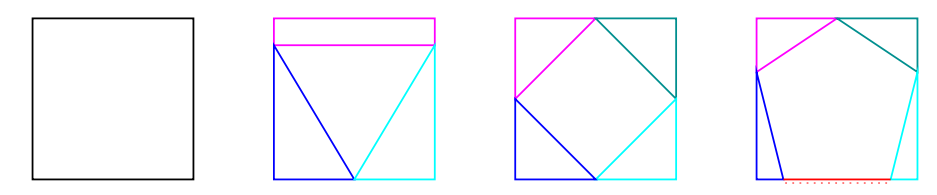
Each partition of \(C\) into \(k\) parts (or, equivalently, each covering of \(C\) by a set of \(k\) minimal closed curves) yields an upper bound for \(\gamma(C,k)\). A few upper bounds on \(\gamma(C,k)\) when \(C\) is a square and \(k \in \{3,4,5\}\) are shown in Figure 1.
Theorem 1.1(Berendsohn, Kim, Kozma [5]).\(\gamma_2(k) \geq \frac{1}{k} + \frac{1}{\pi} \sin \frac{\pi}{k}\). When \(k=2\), this is tight: \(\gamma_2(2) = \frac{1}{2} + \frac{1}{\pi}\).
The lower bound comes from a circle of unit length, in which case the optimal partition consists of equal arcs of length \(1/k\).
They also obtained upper bounds for \(k \geq 2\), by iteratively cutting the closed curve by chords:
\(\gamma_2(a\cdot b) \leq \gamma_2(a) \gamma_2(b)\)
\(\gamma_2(a+b) \leq \big(1 + \frac{2}{\pi}\big) \displaystyle\frac{\gamma_2(a) \gamma_2(b)}{\gamma_2(a) + \gamma_2(b)}.\)
Using these formulas, they obtain the bounds in Table 1. The upper and lower bounds appear to grow increasingly farther apart: by \(k=10\), the bounds differ by a factor of more than 2.5. Indeed, iterated application of either upper bound yields \(\gamma_2(2^n) \leq \gamma_2(2)^n \approx (0.818)^n\), while the lower bound is \(\gamma_2(2^n) \geq \frac{1}{2^n} + \frac{1}{\pi} \sin \frac{\pi}{2^n} \approx 2^{-n+1}\). Under the plausible assumption that the second bound is optimized when \(a=b\) (which is how the upper bounds for all even \(k \leq 10\) are obtained), the ratio between the lower and upper bounds for \(\gamma_2(k)\) grows polynomially with \(k\).
| \(k\) | 1 | 2 | 3 | 4 | 5 | 6 | 7 | 8 | 9 | 10 |
| Lower bound [5] | 1 | \(0.818\) | \(0.609\) | \(0.475\) | \(0.387\) | \(0.325\) | \(0.281\) | \(0.246\) | \(0.220\) | \(0.198\) |
| Upper bound [5] (\(d=2\)) | 1 | \(0.818\) | \(0.737\) | \(0.670\) | \(0.634\) | \(0.603\) | \(0.574\) | \(0.548\) | \(0.533\) | \(0.519\) |
| New upper bound | – | – | \(0.644\) | \(0.494\) | \(0.398\) | \(0.333\) | \(0.285\) | \(0.250\) | \(0.222\) | \(0.200\) |
In [5], the authors propose further investigation of \(\gamma_2(k)\) for \(k\geq 3\) and \(\gamma_d(k)\) for \(d \geq 3\). The starting point for our results is a simple, asymptotically optimal bound for \(\gamma_d(k)\) in all dimensions, which moreover substantially improves the upper bounds for \(\gamma_2(k)\) for all \(k\geq 3\).
Proposition 1.2.\(\gamma_d(k) \leq 2/k\) for all \(k\geq 2\) and \(d \geq 2\).
Because \(\mathbb{R}^2\) embeds in \(\mathbb{R}^d\), Theorem 1.1 implies that \(\gamma_d(k) \geq \gamma_2(k) \geq \frac{1}{k} + \frac{1}{\pi} \sin \frac{\pi}{k}\) for every \(d\) and \(k\); this tends to \(2/k\) as \(k \to \infty\). Therefore \(\gamma_d(k) \sim 2/k\) as \(k\to\infty\) for every \(d\). The remaining additive gap between the lower and upper bounds for \(\gamma_d(k)\) is quite small, namely \(\Theta(k^{-3})\). Still, it would be interesting to know the exact value: is it \(\frac{1}{k} + \frac{1}{\pi}\sin \frac{\pi}{k}\)?
While we do not resolve this question, by using a slightly non-uniform partition of the curve, we do show that the upper bound in Proposition 1.2 can be improved. Our second result is the following.
Theorem 1.3. \(\gamma_d(k) \leq \frac{2}{k}- \frac{1}{4k^4}\) for all \(k\geq 3\) and \(d \geq 2\). Furthermore, for \(k=3,\ldots,10\), \(\gamma_d(k)\) is bounded from above as in row \(3\) of Table 1.
The new upper bounds \(3 \leq k \leq 10\) are obtained by numerically optimizing our argument for those specific values of \(k\).
In the last section, we turn to the problem of computing an optimal \(k\)-covering of a closed polygonal curve. The upper bounds from Berendsohn, Kim, and Kozma, since they’re recursive, could be used to implement a recursive algorithm for this problem. Each recursive call of this algorithm requires identifying a direction in which the width of the curve is small. On the other hand, our proof of Proposition 1.2 gives an almost trivial algorithm: For \(i=0,\ldots,k-1\), take the polygonal arcs between \(x = i/k\) and \(x=(i+1)/k\), and join the endpoints of each arc to make a closed curve. This is a much faster algorithm, of course, and with better approximation ratio. Indeed, any covering of a length-1 curve with closed curves has one curve with length at least \(1/k\), and this algorithm always returns a covering with closed curves, each with length at most \(2/k\). Therefore, this simple algorithm has approximation ratio at most \(2\).
We further improve the ratio \(2\) to \(2 – \frac{1}{4} k^{-3}\), based on Theorem 1.3. For \(k \leq 10\), the approximation ratios are listed below.
| \(k\) | 1 | 2 | 3 | 4 | 5 | 6 | 7 | 8 | 9 | 10 |
| Approximation ratio | \(1\) | \(1.637\) | \(1.932\) | \(1.974\) | \(1.988\) | \(1.993\) | \(1.996\) | \(1.998\) | \(1.998\) | \(2.000\) |
Theorem 1.4. Given a closed polygonal chain \(C=(p_1,p_2,\ldots,p_n)\) in \(\mathbb{R}^d\) and a positive integer \(k \geq 3\), a \(2- \frac{1}{4k^3}\) approximation for covering \(C\) by \(k\) closed curves can be computed in \(O(n+k)\) time. Furthermore, for \(k=3,\ldots,10\), the approximation ratios listed in Table 2 can be obtained.
Estimating the length of a shortest tour of \(n\) points in the unit square with respect to Euclidean distances has been studied as early as the 1940s by Fejes Tóth [11], Few [6], and Verblunsky [12], respectively. Few [6] proved that the (Euclidean) length of a shortest cycle (tour) through \(n\) points in the unit square is at most \(\sqrt{2n}+7/4\). The same upper bound holds for the minimum spanning tree [6]. Karloff [8] derived a slightly better upper bound for the shortest cycle, \(1.392 \sqrt{n} + 7/4\); he also emphasized the difficulty of obtaining further improvements.
Proof of Proposition 1.2. Let \(C\) be any closed curve of length 1, and let \(\mathcal Q\) be a partition of \(C\) into \(k\) connected arcs of \(C\), each of length \(1/k\). Adding the segment joining the endpoints of \(Q \in \mathcal Q\) forms each arc into a closed curve of length at most \(2/k\) (by the triangle inequality), so \(\gamma(C,k) \leq 2/k\). ◻
Proof of Theorem 1.3. Let \(C\) be any closed curve of length 1. Let \[\label{eq:s} s= \frac{1}{k} + (k-1) \varepsilon, \text{ where } \varepsilon= \frac{1}{8k^4}. \tag{3}\]
Our strategy is to take one arc of length \(s\) and split the remaining portion of the curve into \(k-1\) equal-length arcs.
We now find an arc of length \(s\) which can be completed into a short closed curve. To do this, we will use the fact that a circle maximizes the average length of a chord spanning an arc of length \(s\).
Theorem 2.1(Abrams, Cantarella, Fu, Ghomi, and Howard [1]).For any \(s \in [0,1/2]\) and any arc-length parameterization \(r\colon [0,1] \to \mathbb{R}^d\) of a length-1 closed curve, \[\int_0^1 \|r(t+s) – r(t)\|\, dt \leq \frac{\sin{\pi s}}{\pi}.\]
Equality holds if and only if \(r\) parameterizes a circle.
By the series expansion of the \(\sin x\) function around \(x=0\), we have \[\sin x = x – \frac{x^3}{6} + \frac{x^5}{120} \cdots \leq x – \frac{x^3}{12}, \text{ for } x \leq \pi.\]
Theorem 2.1 then implies that there exists an arc \(a_1\) of \(C\) of length \(s\) and which spans a chord of length at most \[\label{eq:a_1} \frac{\sin{\pi s}}{\pi} \leq \frac {\pi s}{\pi} – \frac {\pi^3 s^3}{ 12\pi} = \left( 1 – \frac {\pi^2 s^2}{12} \right) s \leq \left( 1 – \frac{1}{2k^2} \right) s. \tag{4}\]
(Since \(k \geq 3\), we have \(s \leq 1/2\).) Consider the \(k\)-partition of \(C\) into the arc \(a_1\) and \(k-1\) arcs \(a_2,\ldots,a_k\) of the same length \[\frac{1 – s}{k-1}= \frac{1}{k} -\varepsilon,\] which partition \(C \setminus a_1\). We make each arc \(a_i\) (\(i = 1,\dots,k\)) into a closed curve \(C_i\) by adding the segment joining its endpoints.
The length of \(C_1\) is at most \[s + \left( 1 – \frac{1}{2k^2} \right) s = \frac{2}{k} + 2(k-1) \varepsilon- \frac{1}{2k^3} – \frac{(k-1)\epsilon}{2k^2} \leq \frac{2}{k} – \frac{1}{4k^3}.\]
For \(i \geq 2\), the length of \(C_i\) is at most \[\frac{2}{k} – 2\varepsilon= \frac{2}{k} – \frac{1} {4k^4},\] by the triangle inequality. The length of each of the \(k\) curves is therefore bounded above by \[\max \left \{ \frac{2}{k} – \frac{1}{4k^3},\ \frac{2}{k} – \frac{1} {4k^4} \right \} = \frac{2}{k} – \frac{1} {4k^4},\] as claimed.
To obtain specific upper bounds for \(k=3,\ldots,10\), let \(s_k\) be the solution of the equation \[\label{eq:sin} s + \frac{\sin{\pi s}}{\pi} = \frac{2(1-s)}{k-1}. \tag{5}\]
Following the previous argument with \(s_k\) in place of \(s\), we find a covering of \(C\) with \(k\) closed curves, each of length \(2(1-s_k)/(k-1)\). These are the values that appear in Table 1. ◻
In this section we consider closed polygonal curves with regard to the \(k\)-covering problem and prove Theorem 1.4.
Proof of Theorem 1.4. We may assume that \(C\) has unit length. Set \(s = k^{-1} + (k-1) (8k^4)^{-1}\), as in Eq. (3), and consider a moving interval of length \(s\) on \(C\), initially with the left endpoint at a vertex of \(C\).
In the first phase, the algorithm computes an arc \(a_1\) of length \(s\) satisfying inequality (4) by repeatedly advancing a moving arc (interval) counterclockwise on \(C\) stopping at each of the \(2n\) events when passing a segment endpoint, until \(C\) is completely traversed. If the moving interval is contained in a single edge, the scan continues without any computation until the endpoints of the interval are in different chain edges. We therefore obtain a set of at most \(2n\) pairs of equal-length intervals on \(C\), where for each pair, the endpoints of the spanned chord belong to the same pair of edges, say \(e\) and \(e'\), of the chain. The set of interval pairs can be computed in \(O(n)\) time by a linear scan of \(C\).
For each such pair \(I=[a,b], I'=[a',b']\) of intervals on \(C\), compute the corresponding shortest chord and retain the overall shortest one in the end. Overall, the algorithm computes an arc of \(C\) of length \(s\) spanning a chord of minimum length by sequentially examining all possible candidates and retaining the best. See Figure 2 (left).
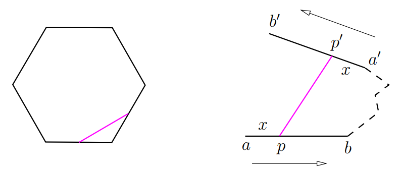
Computing the shortest chord for a given interval pair \(I,I'\), amounts to minimizing a trigonometric function of one variable (the position \(x\) in \(I\)) and that depends solely on the pair of supporting edges \(e,e'\). Specifically, the algorithm computes the solution to the following optimization problem: Given a sequence of four points \(a,b,a',b'\) on \(C\), where \(ab \subset e\), \(a'b' \subset e'\), \(|ab|=|a'b'|\), find \(p \in ab\) and \(p' \in a'b'\), such that \(|ap|=|a'p'|=: x\), and \(|p p'|\) is minimized. See Figure 2 (right). Since \(p\) and \(p'\) move on two lines, the chord length \(|pp'|=|pp'(x)|\) is a unimodal function with a unique minimum for \(x \in [a,b]\).
A solution involves the following steps:
Compute \(|pa'|\) via the Law of Cosines in \(\Delta{pba'}\).
Compute \(\angle{pa'p'}\) via the Law of Sines in \(\Delta{pba'}\).
Compute \(|pp'|\) via the Law of Cosines in \(\Delta{pa'p'}\).
Minimize \(|pp'|\) as a function of \(x\) (check the chords \(aa'\) and \(bb'\) against the one given by the zero of the derivative).
Therefore, computing the solution for a given pair \(I,I'\) of intervals takes \(O(1)\) time. Since there are at most \(2n\) intervals, the first phase takes \(O(n)\) time. In the second phase, the algorithm subdivides the remaining part of the curve into \(k-1\) chains of equal length; this takes \(O(n+k)\) time. Overall, the total time complexity is \(O(n+k)\), as claimed. (For \(k=3,\ldots,10\), \(s\) may be set according to (5) if it yields an improvement.)
To analyze the quality of approximation, one notes that the length of an optimal solution is at least \(1/k\) since we have a covering of \(C\) by \(k\) curves. By Theorem 1.3, the length of each curve in the covering is at most \(2/k -1/(4k^4)\). It follows that the approximation ratio is at most \[\frac{2/k -1/(4k^4)}{1/k} = 2 – \frac{1}{4 k^3},\] as claimed. ◻
Whereas we suspect that the \(k\)-covering problem for closed polygonal curves is \(NP\)-hard, even for curves that are axis-parallel, it is possible that the problem admits better approximations. However, any algorithm that, like ours, computes a set of \(k\) covering curves by partitioning \(C\) into contiguous parts is doomed to avoid the vicinity of an optimal solution in some instances. Let \(\varepsilon>0\) be small. Consider two axis-parallel curves \(C_i\), \(i=1,2\), shown in Figure 3, where the short sides have length \(\varepsilon\). Let \(L_i\), \(i=1,2\), denote the length of each curve.
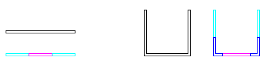
(i) \(C_1\) is a thin axis-parallel rectangle with two sides of unit length; so \(L_1=2+2\varepsilon\). Let \(k=3\). Whereas the covering sketched in Figure 3 (left) achieves \(\gamma(C_1,3) \leq 1/3 + O(\varepsilon)\), any covering obtained by partitioning \(C_1\) into three contiguous parts only achieves \(\gamma'(C_1,3) \geq 1/2- O(\varepsilon)\), where \(\gamma'(C,k)\) stands for \(\gamma(C,k)\) under this restriction. (Note, this inequality is not the best possible, it just involves a simpler argument.)
To see this, one may assume that there is at most one splitting point on the upper side, thus one contiguous part is at least one half of one side, namely \(1/2\), and so the closed curve containing it has length at least \(1\), and the claim follows.
(ii) \(C_2\) is a thin \(U\)-shape with three sides of unit length, two sides of length \(\epsilon\), two sides of length \(1-\varepsilon\) and one side of length \(1-2\varepsilon\); so \(L_2=6 – 2\varepsilon\). Let \(k=5\). Whereas the covering sketched in Figure 3 (right) achieves \(\gamma(C_2,5) \leq 1/5 + O(\varepsilon)\), any covering obtained by partitioning \(C_2\) into five contiguous parts by five splitting points, only achieves \(\gamma'(C_2,5) \geq 1/3- O(\varepsilon)\). The reason for this is that any partition of \(C_2\) into five continuous arcs will have one part that fully contains one of the six long edges. So there is one arc with length at least \(1-2\epsilon\), and the closed curve that contains it has length at least \(2-4\varepsilon\); the claim follows.