
In recent years, with the leaping development of the country’s economic level and standard of living, people’s requirements for food quality are getting higher and higher, and food processing technology is also upgraded [10]. Food processing technology is an important link to ensure food safety and quality, reasonable process design can maximize the retention of food nutrients and taste, while effective regulation methods can prevent food contamination and quality problems [1, 4, 15]. Food process parameter regulation is the basic condition of current food production and quality, and reasonable regulation can improve the quality and taste of food, reduce production costs and food safety risks, improve production efficiency, realize the rational use of resources and protect the environment [2, 6, 18]. In food processing, process parameters include factors such as temperature, time, humidity, concentration, and acid-base value (pH) [13, 16]. The selection and adjustment of these parameters play a vital role in food processing, for example, temperature and time in baked foods can affect the texture and flavor of the product, and too high or too low temperatures may lead to a decrease in the quality of the food [9, 17]. The traditional food processing process has the problems of long processing time, high cost of use and low optimization efficiency [3, 14]. Therefore, how to reasonably set the process parameters and realize the effective regulation of food processing process parameters is an urgent problem to be solved at present.
Multi-objective optimization algorithm is a class of algorithms used to solve optimization problems with multiple objective functions, in the actual problem, there are often multiple conflicting objectives, which requires simultaneous consideration of multiple objectives and find the best compromise between them [21]. The goal of a multi-objective optimization algorithm is to find a set of solutions and make this set of solutions optimal or near-optimal in each objective function [5]. In food processing, multiple process parameters interact with each other, which is equivalent to the conflicting objectives in the multi-objective optimization algorithm, and the optimal solution is achieved in the conflicting objectives, i.e., the optimal regulation of process parameters is obtained.
The traditional optimization methods of food processing process parameters have problems such as high experimental cost, long cycle time and limited optimization accuracy. In this paper, particle swarm algorithm with efficient global search capability and fast convergence characteristics is selected for the optimization of food processing parameters. Aiming at the shortcomings of the particle swarm algorithm, it is improved by combining the adaptive learning factor and the elite particle mutation strategy. The improved particle swarm algorithm is applied to establish the optimization model of kimchi processing parameters. Preprocessing, normalization, abnormal sample test and other operations are carried out on the kimchi processing process data to ensure that the data can be used in the model experiment. Compare the effects of the improved particle swarm algorithm model with those of the particle swarm algorithm model, surface response method and other food processing process parameter optimization methods, and judge the effectiveness of the improved particle swarm algorithm in terms of optimization speed and optimization cost.
To address the problem of regulating the parameters of food processing process, scholars and experts have already conducted research and achieved certain research results. Subramanian et al. [19] reconciled the characterization of aflatoxin under heat treatment in food compounding process by optimizing these parameters of pH, temperature, and time of heat treatment with response surface methodology. Zhang et al. [22] supported by response surface methodology, the optimal parameter ratios of drying temperature, and time, color difference, thickness of yam slices, polysaccharide content and other parameters in drying processing of yam slices were obtained by BP neural network wolf pack (BP-GWO) algorithm. Hussein et al. [7] found that temperature is an important parameter in the process of tomato slices hot-air drying and processing process by Taguchi’s method, while the thickness of the slices has a great impact in the phenomenon of effective moisture diffusion. By regulating the temperature, other parameters such as drying rate and ascorbic acid in the processing can be regulated. Tanash et al. [20] used Taguchi’s method to obtain the optimum value of each parameter, extracted the performance characteristics of each process parameter by orthogonal array and signal-to-noise ratio, and replaced it with the noise ratio to input the fuzzy model, and finally presented it as a composite output index, and the composite output index of each parameter was maximization design as a way to determine the optimal parameter level. In addition, Kothakota et al. [11] used multiple linear regression and artificial neural network (ANN) to optimize the process parameters of nutrient fortification of semolina by treating brown rice with cellulase and xylanase, and setting different treatment parameters and observing the changes of nutrients in semolina after treatment. And Kalathingal et al. [8] set up a model for optimization of process parameters of leaf fluidized bed drying in green tea processing with ANN for inputs (temperature, air flow rate) and outputs (drying time, total color difference, and total phenol content) of parameters in the drying process, and the weights and deviation values of the ANN were calculated by genetic algorithms, so as to obtain the optimal process parameters. Liu et al. [12] set up an optimization model for the process parameters of green tea processing with a Genetic algorithm and particle swarm optimization to optimize the process parameters of vacuum belt drying of orange peels, which not only improves the production efficiency but also reduces the production cost, particle swarm optimization algorithm performs better.
The standard particle swarm (PSO) algorithm has high efficiency and flexibility in solving complex optimization problems, but in some cases there are problems such as easy to fall into local optimum and slow convergence speed. Aiming at the limitations of PSO algorithm, this paper proposes an improved particle swarm algorithm (NIPSO) based on adaptive learning factor (ALF) and elite particle variation strategy (AEM). In the following section, the basic principle of PSO algorithm and its improvement strategy will be introduced in detail, and the application idea of the subsequent NIPSO algorithm in the optimization of food processing process parameters will be clarified.
The idea of the PSO algorithm simulates the process of foraging by group organisms: each individual shares the amount of food at its own location to the group and dynamically pushes the group in the direction of sufficient food based on the experience formed by the amount of food at its own and the group’s location. Figure 1 shows the workflow of the PSO algorithm in synchronization mode. In the engineering application, the PSO algorithm puts \(n\) individual particle with no volume in the Dimensional finite space \(R^{dim}\), and each particle flies with a certain speed in \(R^{dim}\). where the \(i\)th particle has a velocity of \(v_{i} =\left(v_{i,1} \right. ,\left. v_{i,2} ,\ldots ,v_{i,Dim} \right)\) and a position of \(x_{i} =\left(x_{i,l} ,x_{i,2} ,\ldots ,x_{i,Dim} \right)\). The particle’s velocity is dynamically adapted according to its own experience \(pBest_{i}\) and the flight experience of the population formation \(gBest\). The algorithm ends its run when the adaptation of a particle’s position reaches the desired value or reaches the maximum number of runs.
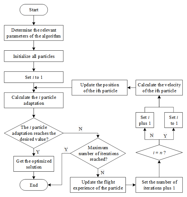
The steps of PSO are as follows:
Step 1: Determine the relevant parameters of the algorithm;
Step 2: Initialize all particles, the initial position and velocity are usually taken as uniformly distributed values, and the velocity can also be taken as zero;
Step 3: Set the value of \(i\) to 1;
Step 4: Calculate the fitness of the \(i\)nd particle position \(Fitness\left(x_{i}^{k} \right)\), the specific fitness formula is related to solve the problem;
Step 5: Judge whether the adaptation degree of the \(i\)th particle position reaches the desired value? If yes, execute Step 6, otherwise execute Step 7;
Step 6: Get the optimized solution \(x_{i,d}^{k}\) whose fitness meets the expected value, and the algorithm finishes running;
Step 7: Determine whether the current number of iterations reaches the maximum number of iterations \(N\), if yes, then the algorithm ends the run, otherwise execute Step 8;
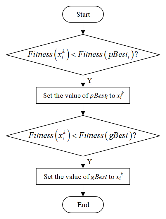
Step 8: update the flight experience of particles, Figure 2 shows the operation flow of updating the flight experience of particles;
Step 9: Add 1 to the number of iterations and add 1 to the value of \(i\) in a loop;
Step 10: Calculate the velocity of the \(i\)nd particle with the velocity update equation: \[\begin{aligned} \label{eq:velocity} {v{}_{i,d}^{k+1} } {=} {\omega v_{i,d}^{k} +c_{1} rand\left[0,1\right]\left(pbest_{i,d}^{k} -x_{i,d}^{k} \right)} {+c_{2} rand\left[0,1\right]\left(gbest_{d}^{k} -x_{i,d}^{k} \right)} , \end{aligned} \tag{1}\] where \(rand\left[0,1\right]\) is the function that generates random numbers in interval \(\left[0,1\right]\).
Step 11: Update the position of the \(i\)rd particle, the position update equation is: \[\label{eq:position} x_{i,d}^{k+1} =x_{i,d}^{k} +v_{i,d}^{k+1} . \tag{2}\]
Jump to step Step 4 to execute.
The particle swarm algorithm No Inertia Velocity Update (NIV) formula is as follows: \[\label{GrindEQ__3_} {v_{i} (t+1)} {=} {s\cdot (u(t)-u(t-1))+c_{1} \times r_{1} \times \left(pbest_{i} (t)-x_{i} (t)\right)} {+c_{2} \times r{}_{2} \times \left(gbest(t)-x_{i} (t)\right)} . \tag{3}\]
Parameter \(s\in (0,1)\) in Eq. (3), referred to as the “coefficient of variation” used to control the range of the population, performs best when it is between \(s\in (0.1,0.2)\). \(u(t)\) and \(u(t-1)\) are the mean values of the positions of the particle swarm at moments \(t\) and \(t-1\). The position update formula definition is consistent with the standard PSO algorithm.
Although the above proposed improved particle swarm algorithm velocity update formula (NIV) can enhance the influence of the optimal position of the swarm on the flight trajectory of the particles, it cannot reduce the possibility of the particles falling into the local optimum. Therefore, on the basis of NIV formula, adaptive learning factor and elite particle variation strategy are introduced to make up for the shortcomings of (NIV) formula and improve the optimization seeking performance of particle swarm algorithm.
The idea of ALF is to linearly adjust the learning factor in the iterative process to guide the direction of particle flight, and in the early stage of the search phase, the particle swarm focuses on the global searched, and in the later stage, it focuses on the fast convergence. The formula for the adaptive learning factor is as follows: \[\label{GrindEQ__4_} c'_{1} =c_{\max } -\frac{\left(c_{\max } -c_{\min } \right)t}{t_{\max } } , \tag{4}\] \[\label{GrindEQ__5_} c'_{2} =c_{\min } +\frac{\left(c_{\max } -c_{\min } \right)t}{t_{\max } } , \tag{5}\] where \(c'_{1}\) decreases linearly with iteration and \(c'_{2}\) increases linearly, and the sum of the two is constant, indicating a certain level of search and convergence of the particle swarm. In the initial stage \(c'_{1} >c'_{2}\) of the algorithm, the particle swarm global search ability is stronger, and in the later stage \(c'_{1} <c'_{2}\) of the algorithm, the particle swarm convergence efficiency is accelerated, which helps the particle swarm to quickly converge to the global optimal solution.
The idea of AEM mutation strategy is to mutate \(gbest(t)\). The current global optimal position can be regarded as the “elite particle” of the particle swarm, and the velocity update formula of the standard particle swarm algorithm is designed to make the particle swarm blindly fly to the elite particle, but this will lead to a large number of aggregation phenomenon of the particle swarm, and it is often difficult for the particle swarm to jump out of the local optimal when the position of the elite particle is the local optimal, so the mutation improvement for \(gbest(t)\) Variation improvement is carried out to break the aggregation phenomenon of the particle swarm, so that it guides the whole particle swarm to jump out of the local optimal solution.
The speed update formula of the improved particle swarm algorithm combining ALF method and AEM strategy is as follows: \[\begin{aligned} \label{GrindEQ__6_} {v_{i} (t+1)} =&{s\cdot (u(t)-u(t-1))+c_{1} {'} \times r_{1} \times \left({\rm \; }pbest_{i} (t)-x_{i} (t)\right)} +c_{2} {'}\notag\\& \times r{}_{2} \times \left(gbest^{*} (t)-x_{i} (t)\right). \end{aligned} \tag{6}\]
The formula for the variation of the AEM strategy for “elite particles” is as follows: \[\label{GrindEQ__7_} gbest^{*} =gbest+G(xm) . \tag{7}\]
From Eq. (7), it can be seen that the elite variant particle \(gbest^{*}\) is only affected by the \(G(xm)\) function and the current population optimal historical position. Where the perturbation function \(G(xm)\) is defined as follows: \[\label{GrindEQ__8_} G\left(xm(i)\right)=\frac{1}{\pi } \arctan \left(xm(i)\right)+C . \tag{8}\]
In Eq. (8), \(i=1,2,\cdots ,N\) is the particle dimension and variables \(xm\) and \(C\) are the two keys in the perturbation function \(G\). Where variable \(C\) takes different values depending on the standard deviation of the particle swarm fitness function values, the specific formula is as follows: \[\label{GrindEQ__9_} C=\left\{\begin{array}{ll} {1.25} & {if{\rm \; }st_{-} d<10^{-2} } ,\\ {1} & {if{\rm \; }10^{-2} \le st_{-} d<10^{-1} } ,\\ {0.25} & {otherwise} , \end{array}\right. \tag{9}\] \[\label{GrindEQ__10_} st_{d} =\sum _{i=1}^{N}\left|\frac{f_{i} -f_{gbest} }{f_{gbest} } \right| , \tag{10}\]
Eq. (9) divides the values into \(\left\{1.25,1,0.25\right\}\) three values, and \(st\_ d\) in Eq. (10) can determine the specific value of \(C\). \(f_{gbest}\) is the value of the fitness function of the historical optimal position of the current population, where \(f_{i}\) indicates the value of the fitness function of the \(i\)th particle, and when \(f_{i}\) tends to be more similar to \(f_{gbest}\), the smaller the value of \(st\_ d\) indicates a higher degree of inter-particle similarity. When the inter-particle similarity is high, variable \(C\) will be given a larger value, which will strengthen the interference effect on \(f_{gbest}\) and break the aggregation of the particle swarm to a certain extent. The formula for variable \(xm\) is defined as follows: \[\label{GrindEQ__11_} xm(i)=\exp \left(-\lambda \cdot t/t_{\max } \right)\cdot \left(1-r(i)/r_{\max } \right) . \tag{11}\]
In Eq. (11), \(\lambda\) is a custom constant, \(t\) is the current number of iterations, \(t_{{\rm max}}\) is the maximum number of iterations, and \(r(i)\) denotes the absolute value of the difference in distance between the \(i\)th dimension of the mean value \(avg\_ pbest\) of the current historical optimal position of all particles and the optimal position of the current population. The definition of \(r(i)\) is shown below: \[\label{GrindEQ__12_} r(i)=\left|gbest(i)-avg\_ pbest(i)\right| , \tag{12}\] where \(avg\_ pbest(i)\) is defined as follows: \[\label{GrindEQ__13_} avg\_ pbest(i)={\left(\sum _{j=1}^{N}p best[j][i]\right)\mathord{\left/ {\vphantom {\left(\sum _{j=1}^{N}p best[j][i]\right) N}} \right.} N} . \tag{13}\]
In Eq. (13), \(pbest[j][i]\) is the value of the \(i\)rd dimension of the \(j\)nd particle at the current historical optimal position. In summary, the improved particle swarm algorithm (NIPSO) is introduced.
In food processing, optimization of process parameters is crucial for improving product quality and production efficiency. As a traditional fermented food, the processing parameters of kimchi affect the final food quality. In order to achieve the optimization of kimchi processing process, this paper constructs a multi-objective parameter optimization model based on the NIPSO algorithm with the objectives of the lowest nitrite content, the maximum crispness of kimchi and the maximum total amount of fresh amino acids. In this part, the construction process of kimchi processing process parameter optimization model will be introduced in detail, and the performance superiority of NIPSO algorithm in the optimization process will be verified through experimental data analysis.
Based on the NIPSO algorithm, the optimization of kimchi processing process parameters is taken as the research object and the corresponding optimization model is constructed. Figure 3 shows the kimchi processing process model. Among them, the main factors on the fermentation of kimchi include salt concentration, temperature, and lactic acid bacteria inoculation amount.
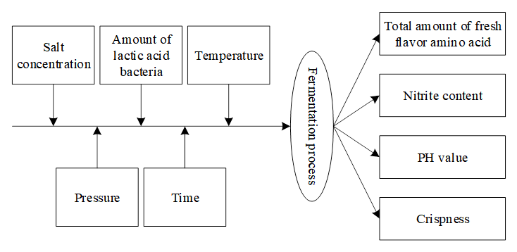
In order to improve the effect of kimchi processing process and realize the optimal process. The salt addition amount, fermentation bacteria inoculation amount, sugar addition amount and fermentation temperature of kimchi were mainly optimized and controlled to achieve the optimal goal.
1) Salt addition amount. The main function of optimizing salt addition is to control microorganisms and harmful bacteria such as fermentation bacteria in kimchi. Different concentrations of salt seriously affect the environmental PH value, and the study combined with experimental experience to control the salt addition in the range of \(0\le S\le 55\%\).
2) Inoculation amount of fermentation bacteria. Different inoculation amount of fermentation bacteria has a large impact on the final acidity of kimchi, therefore, the inoculation amount of fermentation bacteria \(L\) was controlled within the range of 0\(\mathrm{\sim}\)55%.
3) Sugar addition amount. In kimchi processing, the generation of lactic acid bacteria mainly relies on the addition of sugar, and the addition of sugar plays a crucial role for lactic acid bacteria. Therefore, the optimized range of sugar \(U\) was set in the range of 0\(\mathrm{\sim}\)55%.
4) Fermentation temperature. In the fermentation process, the temperature directly affects the microbial content in kimchi, so the fermentation temperature needs to be controlled within a reasonable range. After comprehensive consideration, the fermentation temperature was set to \(25\le T\le 45\).
After clarifying the research object, it is necessary to establish the corresponding objective function. In the optimization of kimchi process, it is mainly divided into two optimization objectives, i.e. single-objective optimization and multi-objective optimization. Single-objective optimization is to take the quality of kimchi as the goal of process optimization, i.e. the final goal of particle swarm optimization.
According to the various influencing factors of kimchi processing, the lowest nitrite content, the maximum crispness of kimchi and the total amount of fresh amino acids were selected as the multi-objective optimization objectives. Its objective function expression is: \[\label{GrindEQ__14_} {J} {c_{1} *\left\| f\left(x_{1} \right)-0\right\| ^{2} +c_{2} *\left\| f_{2} \left(x_{2} \right)-G_{2} \right\| ^{2} } +c{}_{3} *\left\| f_{3} \left(x_{3} \right)-G_{3} \right\| ^{2} . \tag{14}\]
In Eq. (14), \(c_{1}\), \(c_{2}\) and \(c_{3}\) are the weight coefficients of each objective function; \(f_{1} \left(x_{1} \right)\), \(f_{2} \left(x_{2} \right)\) and \(f_{3} \left(x_{3} \right)\) are the models constructed by the objective functions; \(G_{2}\) and \(G_{3}\) are the target values of kimchi crispness and total fresh flavor amino acids, respectively.
This paper utilizes experiments to obtain a total of 23 sets of sample data of relevant parameters of kimchi processing data, in which each set of data contains a complete processing process. The platform used for data processing is Matlab2014a. The preprocessing of the actual test data is realized through the principle of preprocessing technology.
First of all, it is necessary to formulate data cleaning rules, the specific rules are as follows:
1) Analyze the field “salt concentration”, “lactic acid bacteria” and other data, found that the vacant value to eliminate the sample;
2) Compare the field data whether there are duplicates, eliminate duplicate sample data;
In the process of data cleaning, 23 groups of data samples are processed without duplicated data, 1 group of sample data containing empty values is eliminated, and 22 groups of integrated data are obtained.
Table 1 shows some of the experimental test data in this paper. The main purpose of normalization in this paper is to eliminate the influence of the difference of the scale on the results, so this paper adopts the min-max normalization method to normalize the data into the interval of [-1,1]. Observing the experimental test data in Table 1, it can be seen that there is not much difference in the corresponding variable values in each group of data, such as the PH value between 3.64-3.80, which meets the experimental requirements.
| Sample number Variable | 1 | 2 | 3 | 4 | 5 | 6 |
| Salt concentration (%,w/w) | 21 | 16 | 26 | 21 | 16 | 26 |
| Temperature (\(\mathtt{{}^\circ\!{C}}\)) | 26 | 31 | 36 | 36 | 26 | 31 |
| Lactic acid bacteria (%,w/w) | 0.04 | 0.056 | 0.09 | 0.056 | 0.09 | 0.04 |
| Pressure (MPa) | 300 | 300 | 300 | 300 | 300 | 300 |
| Time (min) | 11 | 6 | 16 | 6 | 16 | 11 |
| Nitrite (mg/L) | 2.4 | 1.32 | 2.47 | 2.80 | 1.98 | 2.47 |
| Brittleness (gf) | 1073.34 | 1186 | 1826 | 968.34 | 948.34 | 1636 |
| PH value | 3.64 | 3.64 | 3.80 | 3.67 | 3.65 | 3.70 |
| Total amino acids of umami /nmol/mg | 0.96 | 1.40 | 1.35 | 1.20 | 1.27 | 0.89 |
Finally the data samples are tested for abnormal samples. As the purpose of the detection in this paper is to make the sample data classification more reasonable so as to get a good clustering effect. The rationality evaluation indexes of the samples of the contour method are the number of irrationally categorized samples and the calculated contour value, the fewer the number of irrationally categorized samples, the better, and the closer the average contour value is to 1, the more rational the categorization is. In this subsection, K-mean clustering and contour value calculation are performed for the sample data of 9 variables. The following section takes temperature, pressure, and nitrite as an example to visualize the results of contour value calculation for these three variables and study their optimal number of clusters.
Figure 4 shows the results of contour value calculation under different categories of temperature. Analyzing Figure 4: when the number of categories is 1, the average contour value of all points in the graph is 0.97; when the number of categories is 2, the average contour value of all points in the graph is 0.56; when the number of categories is 3, the contour value of all points in the graph is 1. It indicates that when the number of categories is 3, these points can be well separated from the neighboring clusters. Therefore, the optimal number of clusters for temperature data is 3.
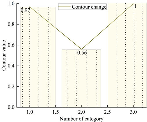
Figure 5 shows the results of calculating the contour values under different categories of pressure. Observing Figure 5, when the number of categories is 1, the average contour value of all the points in the graph is 0.54; when the number of categories is 2, the average contour value of all the points in the graph is 0.76; and when the number of categories is 3, the average contour value of all the points in the graph is 1. It means that when the number of categories is 3, these points can be well separated from the neighboring clusters. Therefore, the optimum number of clusters for the pressure data is 3.
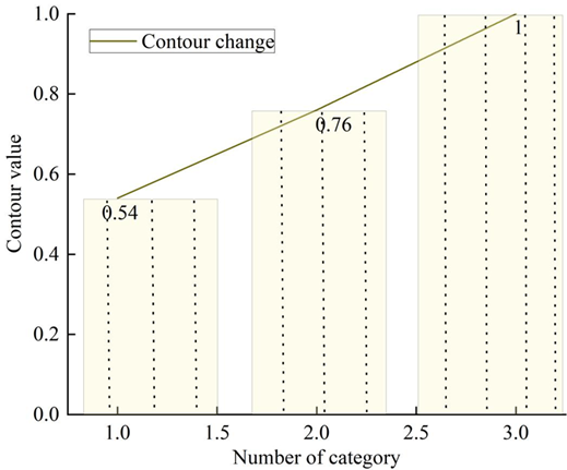
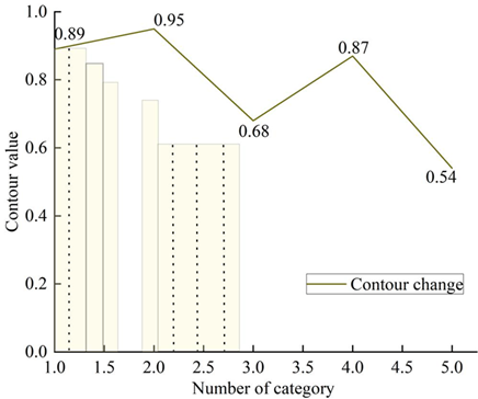
Figure 6 shows the results of calculating the contour values under different categories of nitrite. From Figure 6, when the number of categories is 2, there is no sample point with contour value less than 0 in the graph, indicating that there is no unreasonable categorization. When the classification category is 2, the highest average contour value is 0.95. This indicates that the optimal number of clusters for nitrite data is 2.
Others, the optimal number of clusters for salt concentration, lactic acid bacteria, time, crispness, PH, and total fresh flavor amino acids are 3, 4, 3, 2, 2, 2. After determining the optimal number of clusters, this paper uses the method of K-mean clustering to detect outlier samples for the data of nine variables. The K-mean clustering algorithm to obtain the category attributes of each sample, based on the category attributes to obtain the density of each category, the output of the minimum density of the sample for anomaly analysis, according to the algorithm flow chart, to obtain the mean and standard deviation of the number of elements of each cluster in each category, the number of elements of the cluster with the difference of the mean and the standard deviation of the comparison, to find out that the clusters located in a standard deviation outside of the cluster to look at the set of samples as anomalous samples to be analyzed.
Table 2 shows the minimum density anomaly set elements corresponding to the nine variables.
| Variable value | Set of abnormal samples to be analyzed |
|---|---|
| Salt concentration (%,w/w) | 20 |
| Temperature (\(\mathtt{{}^\circ\!{C}}\)) | 16 |
| Lactic acid bacteria (%,w/w) | 13 |
| Pressure (MPa) | Empty |
| Time (min) | Empty |
| Nitrite (mg/L) | Empty |
| Brittleness (gf) | Empty |
| PH value | Empty |
| Total amino acids of umami /nmol/mg | Empty |
By analyzing the minimum category set, it can be seen that the percentage of salt concentration in sample #20 for salt concentration is 150%, the data clearly defies common sense; while the data for sample #16 for temperature is 350\(^\circ\)C, which is far beyond the temperature range determined by the experiment of obtaining the data, and both of them belong to the obvious entry error data in order to exclude this sample. The detected lactobacilli value of abnormal sample No. 13 was analyzed by professional experimenters, and the values were all within a reasonable experimental range. After the experiment this algorithm misdetects 2 samples. Overall, this paper’s algorithm can more accurately find the abnormal samples to be analyzed, and the processed samples can be used as a data source for subsequent modeling. After pre-processing, the total number of samples remaining 20 groups, randomly selected 15 groups as training sample data, the remaining as a test sample data set, in order to test the generalization ability of the model.
In the calculation and optimization of kimchi processing parameters, the results of temperature, time, and crispness in the processing equipment are used to understand the current operating status of the processing equipment and to predict the degree of parameter optimization that the equipment needs to undergo and the value of the loss that may be caused. The optimization model was used for application scenario testing, and the kimchi processing equipment was subjected to trend analysis under the “N-1” adjustment mode to understand the loss of load of the equipment during the parameter adjustment process. When the particle swarm algorithm before and after the improvement is used for the optimization of parameter adjustment, the basic parameters are set as follows: the number of particles is set to 60, the inertia weight ù = 0.85, the learning factor c\({}_{1}\) = c\({}_{2}\) = 3, and the maximum number of iterations is set to 210.
Figure 7 shows the optimization process of PSO algorithm before and after the improvement to adjust the parameters of the application scenario device. From Figure 7, it can be found that when using the standard PSO algorithm before improvement for equipment parameter adjustment optimization, it has entered the local optimal solution at 52 iterations, and finally after 210 iterations, the result of the optimization converges to the domain of 4,083,300,000 yuan. While using the multi-objective optimization based NIPSO algorithm studied in this paper in 43 iterations, it enters the iterative steady state, and the final convergence domain is 3.509 million yuan.
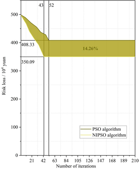
The experimental validation results show that when using the multi-objective optimization based NIPSO algorithm studied in this paper for the optimization of equipment parameter adjustment, it not only reduces the number of iterations from 52 to 43, but also reduces the final risk of loss by 14.26%, which effectively reduces the cost of optimization of kimchi processing parameters.
In order to test whether the multi-objective optimization NIPSO algorithm is more practical than the existing parameter optimization methods, this section takes the surface response method as an example and compares the optimization effects of different methods. In the following section, the optimization process of the surface response method will be studied to determine the practical parameter optimization effect of the two types of methods.
The factors and levels of response surface analysis for kimchi fermentation were designed based on the results of the one-way test, and Table 3 shows the results of the response surface analysis test. Design-Expert 8.0.6 software was used to analyze the data in Table 3 to obtain the model of quadratic multinomial regression equations of total acid content and AITC mass fraction of kimchi on salt addition, fermentation temperature and fermentation time, respectively: \[\begin{aligned} \label{GrindEQ__15_} Y_{1} {\rm =}&1.40{\rm -}4.874{\rm *}10^{{\rm -}3} X_{1} {\rm -}0.094X_{2} {\rm -}0.17X_{3} {\rm +}0.33X_{1} X_{2}\notag\\ &-0.25X_{1} X_{3} -0.071X_{2} X_{3} -0.04X_{1} {}^{2} -0.26X_{2} {}^{2} -0.34X_{3} {}^{2} , \end{aligned} \tag{15}\] \[\begin{aligned} \label{GrindEQ__16_} Y_{2} =&{\rm 0.96+0.22X}_{{\rm 1}} {\rm +0.09X}_{{\rm 2}} {\rm +0.02X}_{{\rm 3}} {\rm +0.36X}_{{\rm 1}} {\rm X}_{{\rm 2}} {\rm +0.36X}_{{\rm 1}} {\rm X}_{{\rm 3}} {\rm +0.01X}_{{\rm 2}} {\rm X}_{{\rm 3}}\notag\\& {\rm +0.09X}_{{\rm 1}} {}^{{\rm 2}} {\rm -0.22X}_{{\rm 2}} {}^{{\rm 2}} {\rm -0.078X}_{{\rm 3}} {}^{{\rm 2}} . \end{aligned} \tag{16}\]
| Test number | X\(_1\) amount of salt added | X\(_2\) fermentation temperature | X\(_3\) fermentation time | Total acid content /(g/kg) | AITC Quality score /% |
| 1 | -1 | 0 | -1 | 0.97 | 1.22 |
| 2 | 0 | 0 | 0 | 1.31 | 1.55 |
| 3 | -1 | 0 | 1 | 1.37 | 1.12 |
| 4 | 0 | 0 | 0 | 1.48 | 0.88 |
| 5 | 0 | 0 | 0 | 1.55 | 0.86 |
| 6 | 1 | 0 | 1 | 1.47 | 0.54 |
| 7 | -1 | 0 | 1 | 1.5 | 0.48 |
| 8 | 0 | 0 | 0 | 1.27 | 1.51 |
| 9 | -1 | -1 | 1 | 0.6 | 0.39 |
| 10 | 0 | -1 | -1 | 1.19 | 0.78 |
| 11 | 1 | 1 | 0 | 1.13 | 0.92 |
| 12 | 1 | -1 | 0 | 0.97 | 0.27 |
| 13 | 0 | 1 | -1 | 0.9 | 0.6 |
| 14 | 0 | 0 | 1 | 0.92 | 0.82 |
| 15 | 1 | 0 | 1 | 0.81 | 0.91 |
Analysis of variance (ANOVA) was performed on the model for total acid content of kimchi. Table 4 shows the ANOVA results of the model of total acid content of kimchi. From Table 4, it can be seen that: the regression model of total acid content of kimchi was highly significant (P<0.01), indicating that the independent variable of the quadratic regression equation was well correlated with the dependent variable; and the misfit was not significant (P=0.5070>0.05), indicating that the equation was a good fit for the test with a small error. The significance of each of the regression equations shows that the primary term X\(_{1}\) is extremely significant (P<0.0001<0.01), X\(_{3}\) is significant (P=0.0240<0.05), and X\(_2\) is not significant (P=0.1459>0.05); the interaction terms X\(_{1}\)X\(_2\), X\(_{1}\)X\(_{3}\) are extremely significant (P<0.0001<0.01), and X\(_2\)X\(_{3}\) is not significant (P=0.4601>0.05); secondary term X\(_2\)\(^{2}\) was significant (P=0.0109<0.05), X\(_{3}\)\(^{2}\) was highly significant (P<0.0001<0.01) and X\(_{1}\)\(^{2}\) was not significant (P=0.4525>0.05). The F-values of X\(_{1}\), X\(_2\) and X\(_{3}\) were 1.174×10\(^{-3}\), 2.04 and 10.19, respectively. According to the size of F-value, the influence of the three factors on the total acid content of kimchi was X\(_{3}\)>X\(_2\)>X\(_{1}\), i.e., fermentation time>fermentation temperature>salt addition, from largest to smallest.
| Source of variation | Sum of squares | Degree of freedom | Mean square | F-number | Prob>F |
|---|---|---|---|---|---|
| Model | 1.40 | 8 | 0.15 | 9.72 | <0.0001** |
| X1 | 1.000×10⁻⁴ | 1 | 1.000×10⁻⁴ | 1.174×10⁻³ | <0.0001** |
| X2 | 0.04 | 1 | 0.035 | 2.04 | 0.1459 |
| X3 | 0.14 | 1 | 0.14 | 10.19 | 0.0240* |
| X1X2 | 0.4 | 1 | 0.4 | 25.5 | <0.0001** |
| X1X3 | 0.26 | 1 | 0.26 | 15.49 | <0.0001** |
| X2X3 | 0 | 1 | 0 | 0.53 | 0.4501 |
| X12 | 0 | 1 | 0 | 0.52 | 0.4525 |
| X22 | 0.23 | 1 | 0.23 | 14.49 | 0.0109* |
| X32 | 0.39 | 1 | 0.39 | 24.69 | <0.0001** |
| Residual error | 0.07 | 4 | 0.01 | ||
| Missing fit | 0.01 | 1 | 3.522×10⁻² | 0.4 | 0.5070 |
| Pure error | 0.04 | 2 | 0.01 | ||
| Total variation | 1.58 | 13 | |||
| Note: * means significant difference (P<0.05), ** means extremely significant difference (P<0.01) | |||||
Analysis of the confidence level of the quadratic regression equation for total acid content shows that the correlation coefficient R\(^{2}\) of the regression equation is 0.9460, which indicates that the equation describes well the relationship between each factor and the response value; The correction coefficient R\(^{2}\)Adj of the regression equation was 0.8486, which indicated that the regression equation could explain 84.87% of the variation of the response value after correction; the signal-to-noise ratio RSN was 8.978, which indicated that the equation had a high goodness-of-fit and credibility, and could be used for the model prediction; and the coefficient of variation CV was 11.43%, which indicated that the regression equation had a high degree of confidence. So the regression equation can be used to optimize the fermentation process of total acid in kimchi.
Analysis of variance (ANOVA) was performed on the model for AITC mass
fraction of kimchi. Table 5 shows the ANOVA
results of the model for AITC mass fraction of kimchi. Analyzing Table
5: The regression model
for AITC mass fraction of kimchi was highly significant
(P<0.0001<0.01) and the misfit was not significant
(P=0.8575>0.05). The significance of each of the regression equations
shows that the primary term X\(_{1}\)
is highly significant (P<0.0001<0.01), X\(_2\) is not significant (P=0.1610>0.05),
and X\(_{3}\) is not significant
(P=0.6485>0.05); the interaction term X\(_{1}\)X\(_2\) is highly significant
(P<0.0001<0.01), X\(_{1}\)X\(_{3}\) is highly significant
(P<0.0001<0.01), and X\(_2\)X\(_{3}\) was not significant
(P=0.8512>0.05); The quadratic term X\(_2\)\(^{2}\) was significant (P=0.0275<0.05),
X\(_{1}\)\(^{2}\) was not significant (P=0.2490
>0.05) and X\(_{3}\)\(^{2}\) was not significant
(P=0.33566>0.05). The F-values of X\(_{1}\), X\(_2\), and X\(_{3}\) were 19.39, 2.54, and 0.22,
respectively. Judging from the magnitude of the F-values, the three
factors affected the AITC mass fraction of total acid in kimchi in
descending order of X\(_{1}\)>X\(_2\)>X\(_{3}\), i.e., the amount of salt
added>fermentation temperature>fermentation time.
| Source of variation | Sum of squares | Degree of freedom | Mean square | F-number | Prob>F |
|---|---|---|---|---|---|
| Model | 1.87 | 8 | 0.20 | 9.98 | <0.0001** |
| X1 | 0.40 | 1 | 0.40 | 19.39 | <0.0001** |
| X2 | 0.04 | 1 | 0.04 | 2.54 | 0.1610 |
| X3 | 4.7×10⁻² | 1 | 4.7×10⁻² | 0.22 | 0.6485 |
| X1X2 | 0.55 | 1 | 0.55 | 26.93 | <0.0001** |
| X1X3 | 0.55 | 1 | 0.55 | 26.93 | <0.0001** |
| X2X3 | 7.9×10⁻⁴ | 1 | 7.9×10⁻³ | 0.03 | 0.8512 |
| X12 | 0.02 | 1 | 0.02 | 1.62 | 0.2490 |
| X22 | 0.16 | 1 | 0.16 | 8.36 | 0.0265* |
| X32 | 0.01 | 1 | 0.01 | 0.99 | 0.3566 |
| Residual error | 0.12 | 5 | 0.01 | ||
| Missing fit | 9.5×10⁻² | 1 | 4.7×10⁻² | 0.16 | 0.8575 |
| Pure error | 0.11 | 3 | 0.02 | ||
| Total variation | 1.99 | 14 | |||
| Note: * means significant difference (P<0.05), ** means extremely significant difference (P<0.01) | |||||
Analysis of the confidence level of the quadratic regression equation for the AITC mass fraction shows that the model has a regression coefficient R\(^{2}\) of 0.9373, a correction coefficient R\(^{2}\)Adj of 0.8435, a coefficient of variation CV of 16.78%, and an RSN signal-to-noise ratio of 11.204. These eigenvalues indicate that the actual prediction test has a small error and a good fit to the model, which can effectively analyze and predict the AITC mass fraction of kimchi.
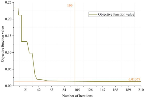
The experimental setup of the surface response method is the same as that of the multi-objective optimization NIPSO algorithm, i.e., the maximum number of iterations is 210, the inertia weights are taken as 0.85, and the learning factors are all 3. The data is prevented from becoming too large for the computation by setting the weights of the three objectives. Figure 8 shows the variation of the scoring value with the number of times. As can be seen from the figure, when the number of iterations reaches 100 times, there is a state of convergence, the convergence of the objective function value of 0.01379, not close to 0, because the ideal value of the three established objective function and the optimal value of the actual situation there is a deviation, in addition, due to the surface response method of the prediction accuracy of the existence of errors and optimization of the objective value of the contradiction between each other. Therefore, the optimized solution is only the relative optimal solution set. Comprehensive analysis shows that the NIPSO algorithm kimchi process parameter optimization model converges at 43 iterations, which is better than the 100 iterations of the surface response method. The surface response method requires more iterations and can only find the relative optimal solution set, which may be caused by the large prediction error of the established multiple regression model on the indicators. Overall, the NIPSO algorithm has a better effect in multi-objective optimization, which can greatly reduce the problems of high cost and long cycle time brought by orthogonal experimental design in the optimization of process parameters, and it can provide an effective reference for practical optimization.
In this paper, for the optimization problem of food processing process parameters, a regulation method based on multi-objective optimization algorithm is proposed, and the optimization research is carried out by improving particle swarm algorithm. After preprocessing, normalization and abnormal sample test of multiple sets of data of kimchi processing, invalid data are eliminated, and the optimal clustering number of each variable is analyzed to be between 2-4 classes, and the final experimental data are obtained. The particle swarm algorithm model before and after the improvement is used to carry out parameter optimization experiments. The number of iterations of the particle swarm algorithm model is 52, and the final convergence domain is 408.33 million yuan. The number of iterations of the improved particle swarm algorithm model is 43, and the final convergence domain is 3.509 million yuan. The number of iterations of the improved particle swarm algorithm model decreases by 9 times and the convergence domain decreases by 14.26%. Compare the improved particle swarm algorithm model with the traditional surface response method. The 43 iterations of the improved particle swarm algorithm model are significantly better than the 100 iterations of the surface response method. The parameter optimization effect of the improved particle swarm algorithm is the best among the three methods.
Using the improved particle swarm algorithm model in this paper can significantly improve the optimization efficiency of kimchi processing parameters, reduce the number of experiments and time costs, and provide more economical and practical optimization solutions for food processing enterprises. As a multi-objective optimization model, the improved particle swarm algorithm model can ensure that multiple key quality variables (e.g., nitrite content, crispness, and the total amount of fresh amino acids, etc.) are optimized simultaneously during the food processing process, which ultimately improves the overall quality of the product and market competitiveness. In the future, the real-time multi-parameter optimization system can be further developed by combining the dynamic data of the actual food processing to adapt to the complex and variable situation of food processing and support the food processing industry to move towards the direction of intelligence.