
The concept of word-representable graphs was introduced by Sergey Kitaev in connection with the study of the Perkins semigroup [30]. Since then, this notion has been widely studied and has found connections to algebra, graph theory, computer science, and combinatorics on words. Word-representable graphs generalise several well-known graph classes, including circle graphs, comparability graphs, and all \(3\)-colourable graphs. These graphs also arise in scheduling problems with repeating tasks, where certain pairs of tasks are required to alternate over time, and these alternation requirements naturally form an undirected graph. A general overview of the background and motivation for studying word-representable graphs is given in [27].
A graph is said to be \(k\)-word-representable if there exists a \(k\)-uniform word representing it. According to Corollary 2.11 and Proposition 2.12, determining whether a graph is word-representable, and whether it is \(k\)-word representable for any given \(3 \leq k \leq \lceil n/2\rceil\), are both NP-complete problems. From a \(k\)-word representation of a word-representable graph, one can derive an upper bound on the representation number of the graph. Therefore, it is important to study the word-representability of specific graph classes and to obtain polynomial-time bounds on their representation numbers.
Word-representability and representation numbers have been studied for several classes of graphs. In [28], outerplanar graphs and prism graphs were shown to be word representable, while odd wheel graphs were proved to be non-word representable. The word-representability of crown graphs and \(k\)-cube graphs was investigated in [19] and [9], respectively. The representation number of crown graphs was determined in [19], where it was shown that the crown graph \(H_{k,k}\) has representation number \(\lceil k/2 \rceil\). More recently, Hefty et al. [22] established several lower bounds on the representation numbers of various graph classes, including balanced bipartite graphs, hypercubes, and comparability graphs. The word-representability of split graphs was studied in [23, 26, 24, 11]. In [16], it was shown that the representation number of any word-representable split graph is at most three. In particular, [29] studied the word-representability of split graphs using vertex labelling and also provided a polynomial-time recognition algorithm for word-representable split graphs. In [14], the authors established necessary and sufficient conditions for a co-bipartite graph to be word-representable based on orientation. In [10], the authors explored \(K_m\)–\(K_n\) graphs (co-bipartite graphs) and identified forbidden induced subgraphs for \(K_m\)–\(K_3\) and \(K_m\)–\(K_4\). Later, a necessary and sufficient vertex-ordering characterisation of word-representable co-bipartite graphs was obtained in [15]. Vertex-ordering characterisations have been widely used to obtain forbidden-pattern characterisations of several important graph classes, including interval graphs, permutation graphs, and comparability graphs. For example, a graph \(G\) is an interval graph if and only if there exists a vertex ordering such that, for any three vertices \(x \prec y \prec z\), adjacency of \(x\) and \(z\) implies adjacency of \(y\) and \(z\) [32]. Additional significant results on forbidden-pattern characterisations can be found in [13, 18] and [7, Section 7.4].
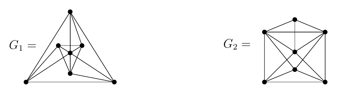
The class of co-bipartite graphs contains both word-representable and non-word representable graphs. In particular, the graphs \(G_1\) and \(G_2\) are minimal, with respect to the number of vertices, non-word-representable co-bipartite graphs, as shown in Figure 1.
The classes of split graphs and co-bipartite graphs are hereditary, since every induced subgraph of a graph in either class also belongs to the same class. Split graphs and co-bipartite graphs play an important role in the study of the speed of hereditary graph classes and their asymptotic structure, and these aspects have been extensively studied in the literature. These concepts are also closely related to the asymptotic enumeration of word-representable graphs, as discussed in [12]. In general, for every infinite hereditary class \(X\) of simple graphs, the following holds: \[\lim_{n\to\infty}\frac{\log_2 X_n}{\binom{n}{2}} = 1 – \frac{1}{k(X)},\] where \(k(X)\) is called the index of \(X\). This index is defined using the graph classes \({\cal E}_{i,j}\), consisting of graphs whose vertices can be partitioned into at most \(i\) independent sets and \(j\) cliques. In particular, bipartite graphs, split graphs, and co-bipartite graphs correspond to the classes \({\cal E}_{2,0}\), \({\cal E}_{1,1}\), and \({\cal E}_{0,2}\), respectively. The index \(k(X)\) is the maximum integer \(k\) such that \(X\) contains the class \({\mathcal E}_{i,j}\) for some integers \(i\) and \(j\) satisfying \(i + j = k\). This result was independently established by Alekseev [1] and by Bollobás and Thomason [5, 6], and is now known as the Alekseev–Bollobás–Thomason Theorem (see also [2]). Recent work by Feng et al. [17] established a general framework for proving factorial speed via finite-language graph representations. This approach provides a powerful tool for establishing the factorial speed of hereditary graph classes and has been used to show that several graph classes have at most factorial speed.
Since co-bipartite graphs are complements of bipartite graphs, they can be recognised in polynomial time. Furthermore, several computational problems that are difficult for general graphs admit polynomial-time algorithms when restricted to co-bipartite graphs. For example, Brandstädt et al. [8] gave a polynomial-time algorithm to determine whether a graph contains a stable set whose removal results in a co-bipartite graph. Similarly, the \(cd\)-coloring problem can be solved in polynomial time for co-bipartite graphs [33]. However, not all computational problems become easier on this class. Bodlaender and Jansen [3] showed that the SIMPLE MAX CUT problem remains NP-complete for co-bipartite graphs. Moreover, the class of co-bipartite graphs has unbounded clique-width and contains at least \(2^{n^2/4}\) distinct graphs on \(n\) vertices [4].
The study of word-representability of co-bipartite graphs is natural in the context of graph classes defined by vertex partitions. Bipartite graphs, where the vertex set can be partitioned into two independent sets, and split graphs, where the vertex set can be partitioned into one clique and one independent set, have already been studied in the context of word-representability. Co-bipartite graphs, where the vertex set can be partitioned into two cliques, form the complementary class of bipartite graphs. Therefore, it is natural to study the word-representability of co-bipartite graphs.
A necessary and sufficient condition for word-representable co-bipartite graphs in terms of a vertex ordering was established in [15]. Using this ordering, we present a constructive algorithm for obtaining a \(3\)-uniform word-representation of every word-representable co-bipartite graph, thereby establishing that its representation number is at most \(3\). Furthermore, we prove that a word-representable co-bipartite graph has representation number \(3\) if and only if it is not a permutation graph. Since the class of word-representable graphs is hereditary, the class of word-representable co-bipartite graphs is also hereditary. We also determine the speed and entropy of the class of word-representable co-bipartite graphs, showing that its speed is at most \(2^{O(n\log n)}\) and its entropy is \(0\). Thus, vertex ordering serves as an effective tool for studying the structural and combinatorial properties of word-representable co-bipartite graphs.
The main goal of this paper is to study the word-representability of co-bipartite graphs via vertex ordering. In Section 2, we introduce the necessary definitions and preliminaries related to word-representable graphs. In Section 3, based on the vertex ordering of word-representable co-bipartite graphs [15], we present an algorithm that constructs a \(3\)-uniform word-representation for any word-representable co-bipartite graph. In Section 4, we study the speed and entropy of the class of word-representable co-bipartite graphs.
In this section, we briefly describe the necessary definitions, notation, and basic results on word-representable graphs.
A simple graph \(G(V, E)\) is an undirected graph with a vertex set \(V\) and an edge set \(E\). For a vertex \(v \in V\), \(N_v\) denotes the set of vertices in \(V\) that are adjacent (neighbours) to \(v\). The degree of a vertex \(v\) is defined as the cardinality of \(N_v\). A subset \(S \subseteq V\) is called an independent set if no two distinct vertices \(u, v \in S\) are adjacent. A subset \(C \subseteq V\) is called a clique if every pair of distinct vertices \(u, v \in C\) is adjacent. A clique \(C\) is said to be maximal if there is no vertex \(v \in V \setminus C\) such that \(C \cup \{v\}\) is also a clique in \(G\).
For a graph \(G(V,E)\), let \(V^{+}\) denote the set of all nonempty words over the alphabet \(V\). Suppose \(w\) is a word over an alphabet \(V\). Two distinct letters \(x\) and \(y\), with \(x,y \in V\), are said to alternate in the word \(w\) if, after deleting all letters in \(w\) except the occurrences of \(x\) and \(y\), the resulting word is of the form \(xyxy\cdots\) or \(yxyx\cdots\) (of either odd or even length). Both \(x\) and \(y\) must appear at least once in \(w\) for alternation to occur. If \(x\) and \(y\) do not alternate in \(w\), then \(x\) and \(y\) are called non-alternating in \(w\).
Definition 2.1 ([27] , Definition 3.0.5). A simple graph \(G(V, E)\) is word-representable if there exists a word \(w\) over the alphabet \(V\) such that letters \(x\) and \(y\), where \(x\neq y\) and \(x,y\in V\), alternate in \(w\) if and only if \(x\) and \(y\) are adjacent in \(G\). If a word \(w\) represents \(G\), then \(w\) contains each letter of \(V\) at least once.
Definition 2.2 ([27], Definition 3.2.1.). A \(k\)-uniform word is a word \(w\) in which every letter occurs exactly \(k\) times.
Definition 2.3 ([27], Definition 3.2.3.). A graph is \(k\)-word-representable (or \(k\)-representable) if there exists a \(k\)-uniform word representing it.
Theorem 2.4 ([28], Theorem 7). A graph \(G\) is word-representable if and only if there exists an integer \(k\ge 1\) such that \(G\) is \(k\)-representable.
Definition 2.5 ([25], Definition 3). For a word-representable graph \(G\), the representation number is the least \(k\) such that \(G\) is \(k\)-representable.
For a circle graph, the representation number is already known.
Theorem 2.6 ([25], Theorem 6). \[\mathcal{R}_2 = \{G: G \text{ is a non-complete circle graph}\}.\]
Proposition 2.7 ([27], Proposition 3.0.15). Let \(w = w_1xw_2xw_3\) be a word representing a graph \(G\), where \(w_1\), \(w_2\) and \(w_3\) are possibly empty words, and \(w_2\) contains no \(x\). Let \(X\) be the set of all letters that appear only once in \(w_2\). Then, possible candidates for \(x\) to be adjacent in \(G\) are the letters in \(X\).
The initial permutation of \(w\) is the permutation obtained by removing all but the leftmost occurrence of each letter \(x\) in \(w\), and it is denoted by \(\pi(w)\). Similarly, the final permutation of \(w\) is the permutation obtained by removing all but the rightmost occurrence of each letter \(x\) in \(w\), and it is denoted \(\sigma(w)\). For a word \(w\), \(w_{\{x_1, \cdots, x_m\}}\) denotes the word after removing all letters except the letters \(x_1, \ldots, x_m\) present in \(w\).
Example 2.8. \(w = 6345123215\), we have \(\pi(w) = 634512\), \(\sigma(w) = 643215\) and \(w_{\{6,5\}} = 655\).
There exists a connection between graph orientations and word-representability. In the following, the definition of a semi-transitive orientation and its connection to word-representability are described.
Semi-transitive orientation is defined based on shortcuts in the papers [20] and [21]. A semi-cycle is the directed acyclic graph obtained by reversing the direction of one edge of a directed cycle [27]. An acyclic digraph is a shortcut if it is induced by the vertices of a semi-cycle and contains a pair of non-adjacent vertices. Thus, any shortcut
is acyclic (that is, there are no directed cycles);
has at least 4 vertices;
has exactly one source (the vertex with no edges coming in), exactly one sink (the vertex with no edges coming out), and a directed path from the source to the sink that goes through every vertex in the graph;
has an edge connecting the source to the sink that we refer to as the shortcutting edge;
is not transitive (that is, there exist vertices \(u\), \(v\) and \(z\) such that \(u\rightarrow v\) and \(v\rightarrow z\) are edges, but there is no edge \(u\rightarrow z\)).
Definition 2.9. [21] An orientation of a graph is semi-transitive if it is acyclic and shortcut-free.
From these definitions, it is clear that any transitive orientation is necessarily semi-transitive. The converse is not true. Thus, semi-transitive orientations generalise transitive orientations. A key result in the theory of word-representable graphs is the following theorem.
Theorem 2.10 ([21], Theorem 3). A graph is word-representable if and only if it admits a semi-transitive orientation. Moreover, each non-complete word-representable graph is \(2(n-\kappa)\)-word-representable where \(\kappa\) is the size of the maximum clique in \(G\).
The recognition problem of word-representable graphs and deciding the representation number of word-representable graphs are \(NP\)-complete problems.
Corollary 2.11 ([21], Corollary 2). The recognition problem for word-representable graphs is NP-complete.
Proposition 2.12 ([21], Proposition 8.). Deciding whether a given graph is a \(k\)-word-representable graph, for any given \(3 \leq k \leq \lceil n/2\rceil\), is NP-complete.
The following characterisation of word-representable split graphs is derived using vertex labelling. In what follows, for any two integers \(a \le b\), we denote the set of integers \(\{a, a+1, \ldots, b\}\) by \([a, b]\).
Theorem 2.13. [29] Let \(G (I \cup C, E)\) be a split graph. Then, \(G\) is word-representable if and only if the vertices of \(C\) can be labelled from \(1\) to \(k = |C|\) in such a way that for each \(a, b \in I\) the following holds.
A word \(u\) contains a word \(v\) as a factor if \(u = xvy\) where \(x\) and \(y\) can be empty words. In this paper, \(w=w_1w_2\cdots w_n\) denotes the word \(w\) contains \(\{w_1,w_2,\ldots, w_n\}\) as factors where \(w_i\) is a word possibly empty. In a graph \(G(V,E)\), we denote the edges between two vertices \(x\) and \(y\) as \(x \sim y\). If there is no edge between them, we denote this as \(x \nsim y\).
Since co-bipartite graphs are complements of bipartite graphs, let \(B(X,Y)\) denote a bipartite graph with independent sets \(X\) and \(Y\), where \(|X|=m\), \(|Y|=n\), and \(X\) is the larger independent set. We denote its complement, i.e., the co-bipartite graph, by \(\overline{B}(K_m,K_n)\), where \(K_m=\overline{B}[X]\) and \(K_n=\overline{B}[Y]\) are cliques. Thus, two vertices are adjacent in \(\overline{B}(K_m,K_n)\) if and only if they are non-adjacent in \(B(X,Y)\). Since \(X\) is chosen as the larger independent set in \(B(X,Y)\), every apex vertex (a vertex adjacent to all other vertices) of \(\overline{B}(K_m,K_n)\) belong to the maximal clique \(K_m\).
The word-representability of co-bipartite graphs is studied in [14], where necessary and sufficient conditions for semi-transitive orientations of co-bipartite graphs are established. The known results concerning the semi-transitive orientation of co-bipartite graphs are as follows.
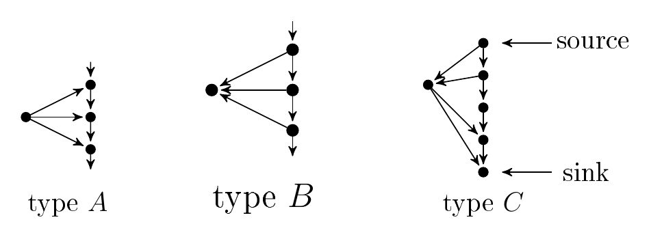
Observation 2.14. [14] Any semi-transitive orientation of \(\overline{B}(K_m,K_n)\) subdivides the set of all vertices into three possibly empty groups of the types shown schematically in Figure 2.
The vertical oriented paths are a schematic way to show (parts of) \(\vec{P_1}\) for \(V(K_m)\) and \(\vec{P_2}\) for \(V(K_n)\);
For the vertices of \(K_m\), the vertical oriented paths in the types \(A\) and \(B\) represent up to \(l\) consecutive vertices in \(\vec{P_1}\), \(l\leq n\). Similarly, for the vertices of \(K_n\), the vertical oriented paths in the types \(A\) and \(B\) represent up to \(l\) consecutive vertices in \(\vec{P_2}\), \(l\leq m\).
For the vertices of \(K_m\), the vertical oriented path in type \(C\) contains all \(n\) vertices in \(\vec{P_1}\). Similarly, for the vertices of \(K_n\), the vertical oriented path in type \(C\) contains all \(m\) vertices in \(\vec{P_2}\). These oriented paths \(P_1\) and \(P_2\) are subdivided into three groups of consecutive vertices, with the middle group possibly containing no vertices; the group of vertices containing the source (resp., sink) is the source-group (resp., sink-group).
Lemma 2.15. [14] Suppose that the graph \(\overline{B}(K_m,K_n)\) is word-representable and \(S\) is a semi-transitive orientation of the graph \(\overline{B}(K_m,K_n)\). Suppose \(\{x,y\}\in V(K_m)\) and \(x\) is a type \(A\) vertex and \(y\) is a type \(B\) vertex and the orientation of the edge between \(x\) and \(y\) is \(y\rightarrow x\). Then, \(x\) and \(y\) do not have any common neighbour among the vertices of \(K_n\).
Lemma 2.16. [14] Suppose the graph \(\overline{B}(K_m,K_n)\) is word-representable and \(S\) is a semi-transitive orientation of the graph \(\overline{B}(K_m,K_n)\). Suppose \(\{x,y\}\in V(K_m)\) and \(\{x_s,x_{s+1}\}\in V(K_n)\), and the orientation of the edges between \(\{x,y\}\) is \(x \rightarrow y\), and between \(\{x_s,x_{s+1}\}\) is \(x_s \rightarrow x_{s+1}\) in the semi-transitive orientation \(S\). Then, the semi-transitive orientation \(S\) follows the following conditions:
Lemma 2.17. [14] Suppose the graph \(\overline{B}(K_m,K_n)\) is word-representable and \(S\) is a semi-transitive orientation of the graph. Let \(x\in V(\overline{B}(K_m,K_n))\), and \(x\) is a type \(C\) vertex. Suppose \(x_s\) and \(x_{s+1}\) are the last and first vertices of the source and sink group, respectively. Now, for \(y\in V(\overline{B}(K_m,K_n))\), if \(x\) and \(y\) are in the same partition in the graph \(V(\overline{B}(K_m,K_n))\), then the following conditions hold for \(y\).
If the edges between \(x\) and \(y\) are oriented as \(y\rightarrow x\), \(y\) is not a type \(B\) vertex that is adjacent to both \(x_s\) and \(x_{s+1}\). Also, if \(y\) is a type \(C\) vertex, then \(x_{s+1}\) cannot be contained in the source group of \(y\).
Theorem 2.18. [14] A co-bipartite graph \(\overline{B}(K_m,K_n)\) has a semi-transitive orientation if and only if
\(K_m\) and \(K_n\) are oriented transitively,
In the graph \(\overline{B}(K_m,K_n)\), every vertex belongs to one of the three types described in Observation 2.14, and
The conditions present in Lemmas 2.15, 2.16 and 2.17 are satisfied.
In the paper [15], a necessary and sufficient condition for a word-representable co-bipartite graph is derived based on the vertex ordering obtained from Observation 2.14. In the following theorems, we denote the neighbours of a type \(A\) or \(B\) vertex \(a_i\) (excluding the vertices of \(K_m\)) as \([x_i,y_i]=\{x_i,x_{i+1},\ldots, y_{i-1},y_i\}\), where \(\{x_i,x_{i+1},\ldots, y_{i-1},y_i\}\subseteq V(K_n)\) and the neighbour of type \(C\) vertex \(c_i\) (excluding the vertices of \(K_m\)) as \([1,x_i]\cup[y_i,n]=\{1,2,\ldots,x_i,y_i,\ldots,n\}\), where \(\{1,2,\ldots,x_i,y_i,\ldots,n\}\subseteq V(K_n)\).
Theorem 3.1. [15] A co-bipartite graph \(\overline{B}(K_m,K_n)\), where \(V(K_n)=\{1,2,\ldots,n\}\), is word-representable if and only if there exists a vertex ordering for the vertices of \(K_m\) that satisfies the following conditions:
Suppose \(c_i\) and \(c_j\) are type \(C\) vertices, \(c_i<c_j\), \(c_i,c_j\in V(K_m)\). Let \(N_{c_i}\setminus V(K_m)=[1,x_i]\cup [y_i,n]\), \(N_{c_j}\setminus V(K_m)=[1,x_j]\cup [y_j,n]\). Then \(x_i\leq x_j\) and \(y_i\leq y_j\).
Suppose \(a_i\) and \(a_j\) are type \(A\) or type \(B\) vertices, \(a_i<a_j\), \(a_i,a_j\in V(K_m)\). Let \(N_{a_i}\setminus V(K_m)=[x_i,y_i]\), \(N_{a_j}\setminus V(K_m)=[x_j,y_j]\). Then \(x_i\leq x_j\) and \(y_i\leq y_j\).
Suppose \(a_i\) is type \(A\) (or \(B\)) vertex and \(c_j\) is type \(C\) vertex, \(a_i<c_j\)(or \(a_i>c_j\) for type \(B\)), \(a_i,c_j\in V(K_m)\). Let \(N_{a_i}\setminus V(K_m)=[x_i,y_i]\), \(N_{c_j}\setminus V(K_m)=[1,x_j]\cup [y_j,n]\). Then \(x_i\leq y_j\) and \(x_j\leq y_i\).
Suppose \(a_i\) is type \(A\) vertex and \(b_j\) is type \(B\) vertex. Let \(N_{a_i}\setminus V(K_m)=[x_i,y_i]\), \(N_{b_j}\setminus V(K_m)=[x_j,y_j]\). Then \(x_j\leq x_i\) and \(y_j\leq y_i\).
Suppose \(v\in V(K_m)\) and \(N_v\setminus V(K_m)=\emptyset\). Let \(a_i\) be the last type \(A\) vertex and \(c_j\) be any type \(C\) vertex. Then \(a_i<v<c_j\) and \(y_i<y_j\), where \(N_{a_i}\setminus V(K_m)=[x_i,y_i]\), \(N_{c_j}\setminus V(K_m)=[1,x_j]\cup [y_j,n]\).
From the labelling conditions, we observe that only type \(A\) and type \(C\) vertices are enough to obtain a semi-transitive orientation. In the following theorem, we prove this statement.
Theorem 3.2. [15] Let \(G\) be a word-representable co-bipartite graph, and let \(S\) be a semi-transitive orientation of \(G\) containing vertices of types \(A\), \(B\), and \(C\). Then \(G\) admits another semi-transitive orientation in which every vertex is of either type \(A\) or type \(C\), and no vertex is of type \(B\).
We determine the maximum possible representation number of a co-bipartite graph using the ordering obtained from Theorems 3.1 and 3.2. We show that this number is at most 3 by providing an algorithm that constructs a \(3\)-word representation for any word-representable co-bipartite graph. In this algorithm, we take the matrix \(M_{m \times n}\) as input, described below.
\(M_{m\times n}\) is a matrix representation of the co-bipartite graph \(\overline{B}(K_m,K_n)\) where
the rows of \(M_{m\times n}\) correspond to the vertices of \(K_m\),
the columns of \(M_{m\times n}\) correspond to the vertices of \(K_n\), and
\(M[i][j]=\begin{cases} 1, \text{ if } i\sim j\\ 0, \text{ otherwise } \end{cases}\)
In the matrix \(M_{m\times n}\), we define two types of vertices, where \(1\leq j\leq n\).
If \(a\) is a type \(A\) vertex then, it is represented as \([x_i,y_i]\) where \[M_{a\times j}=\begin{cases} 1, \text{ if } x_i\leq j\leq y_i,\\ 0, \text{ otherwise}. \end{cases}\]
If \(c\) is a type \(C\) vertex then, it is represented as \([1,x_i]\cup [y_i,n]\) where \[M_{c\times j}=\begin{cases} 1, \text{ if } 1\leq j\leq x_i,\\ 1, \text{ if } y_i\leq j\leq n, \\ 0, \text{ otherwise}. \end{cases}\]
One key point to note is that any vertex \(v\) with \(v \in V(K_m)\) and \(N_v \setminus V(K_m) = \varnothing\) is treated as a type \(A\) vertex in the algorithm.
Theorem 3.3. The representation number of word-representable co-bipartite graphs is at most \(3\).
Proof. We provide an algorithm to generate a \(3\)-uniform word that represents a word-representable co-bipartite graph. The construction starts with three identical permutations of the vertices of \(K_n\). Vertices of \(K_m\) are inserted so that each vertex alternates exactly with its neighbourhood interval. Type \(C\) vertices are inserted first to preserve the nesting of neighbourhoods, followed by type \(A\) vertices inserted according to the ordering constraints of Theorem 3.1. This guarantees a valid \(3\)-uniform word-representation.
Algorithm (Word-representation of a word-representable co-bipartite graph).
Our claim is that the word obtained from the algorithm is a word-representation of the word-representable co-bipartite graph.
Proof of Correctness
We prove that the algorithm returns a \(3\)-uniform word representing the given word-representable co-bipartite graph \(G\).
Step 1: Each vertex occurs exactly three times.
Initially, \(w=P_1P_2P_3\), where \(P_1=P_2=P_3=P\). Therefore, every vertex of \(K_n\) occurs exactly once in each of \(P_1\), \(P_2\), and \(P_3\), and hence exactly three times in \(w\).
Now consider a vertex of \(K_m\).
Suppose \(c_i\) is a type \(C\) vertex. The algorithm inserts one occurrence of \(c_i\) into each of \(P_1\), \(P_2\), and \(P_3\). Later, if the first occurrence of \(c_i\) is removed from \(P_1\), it is immediately reinserted as part of the block \(c_1c_2\cdots c_j\) in the same copy \(P_1\). Hence, no occurrence of \(c_i\) is lost or duplicated, and therefore \(c_i\) occurs exactly three times in the final word.
Suppose \(a_i\) is a type \(A\) vertex. The algorithm inserts one occurrence of \(a_i\) after \(y_i\) in \(P_1\), one occurrence after \(y_i\) in \(P_2\), and one occurrence before \(x_i\) in \(P_1\). In the case \(y_{i-1}<x_i\), the second occurrences of the previously inserted type \(A\) vertices are removed and immediately reinserted before \(x_i\). Consequently, no occurrence of any type \(A\) vertex is lost or duplicated. Hence, every type \(A\) vertex also occurs exactly three times in the final word.
Therefore, every vertex of \(G\) appears exactly three times in the final word. Since no vertex appears more or fewer than three times, the output word is \(3\)-uniform.
Step 2: Every edge corresponds to alternation.
We now show that if \(u\) and \(v\) are adjacent in \(G\), then \(u\) and \(v\) alternate in the final word.
Two vertices of \(K_n\).
Since \(w_{V(K_n)}=P_1P_2P_3=P^3\), for any two vertices \(u,v\in V(K_n)\), we have \(w_{\{u,v\}}=uvuvuv\) or \(w_{\{u,v\}}=vuvuvu\). Hence, every pair of vertices of \(K_n\) alternates.
A type \(A\) vertex and a vertex of \(K_n\).
Let \(a_i\) be a type \(A\) vertex with \(N_{a_i}\setminus V(K_m)=[x_i,y_i]\). The algorithm places one occurrence of \(a_i\) before \(x_i\) in \(P_1\) and the remaining two occurrences after \(y_i\) in \(P_1\) and \(P_2\). Therefore, for every vertex \(u\in [x_i,y_i]\), we obtain \(w_{\{a_i,u\}}=a_iua_iua_iu\). Hence, \(a_i\) alternates with every vertex of its neighbourhood.
A type \(C\) vertex and a vertex of \(K_n\).
Let \(c_i\) be a type \(C\) vertex with \(N_{c_i}\setminus V(K_m)=[1,x_i]\cup [y_i,n]\). The algorithm inserts the occurrences of \(c_i\) after the first and second occurrences of \(x_i\) and before the third occurrence of \(y_i\). Therefore, for every vertex \(u\in [1,x_i]\cup [y_i,n]\), we obtain \(w_{\{c_i,u\}}=c_iuc_iuc_iu\) or \(w_{\{c_i,u\}}=uc_iuc_iuc_i\). Hence, \(c_i\) alternates with every vertex of its neighbourhood.
Two vertices of \(K_m\).
Suppose \(u=a_i\) and \(v=a_j\) are type \(A\) vertices. By Theorem 3.1, \(x_i\le x_j\) and \(y_i\le y_j\).
If \(y_i\ge x_j\), then the occurrences of \(a_i\) and \(a_j\) are naturally interleaved, and \(w_{\{a_i,a_j\}}=a_ia_ja_ia_ja_ia_j\).
If \(y_i<x_j\), the algorithm relocates the second occurrence of \(a_i\) immediately after the first occurrence of \(a_j\). Consequently, \(w_{\{a_i,a_j\}}=a_ia_ja_ia_ja_ia_j\).
Hence, \(a_i\) and \(a_j\) alternate.
Suppose \(u=c_i\) and \(v=c_j\) are type \(C\) vertices. By Theorem 3.1, \(x_i\le x_j\) and \(y_i\le y_j\). Since the insertion rule preserves this nesting, \(w_{\{c_i,c_j\}}=c_ic_jc_ic_jc_ic_j\) or its reverse. Therefore, \(c_i\) and \(c_j\) alternate.
Suppose \(u=a_i\) and \(v=c_j\). By Theorem 3.1, \(x_i\le y_j\) and \(x_j\le y_i\).
If \(x_i\le x_j\), then \(w_{\{a_i,c_j\}}=a_ic_ja_ic_ja_ic_j\).
If \(x_i>x_j\), the first occurrences of the type \(C\) vertices are relocated before inserting \(a_i\), and again \(w_{\{a_i,c_j\}}=a_ic_ja_ic_ja_ic_j\).
Hence, \(a_i\) and \(c_j\) alternate.
Therefore, every edge of \(G\) corresponds to alternation.
Step 3: Every non-edge corresponds to non-alternation.
We now show that if \(u\) and \(v\) are non-adjacent in \(G\), then \(u\) and \(v\) do not alternate in the final word.
Non-neighbours of a type \(A\) vertex.
Let \(a_i\) be a type \(A\) vertex with \(N_{a_i}\setminus V(K_m)=[x_i,y_i]\).
For every vertex \(u\in \{1,\ldots ,x_i-1\}\), we have \(w_{\{a_i,u\}}=ua_ia_iua_iu\), which contains the factor \(a_ia_i\). Hence, \(a_i\) and \(u\) do not alternate.
For every vertex \(v\in \{y_i+1,\ldots ,n\}\), if the second occurrence of \(a_i\) is not relocated, then \(w_{\{a_i,v\}}=a_ia_iva_ivv\), which contains the factor \(a_ia_i\) or \(vv\).
If the second occurrence of \(a_i\) is relocated in Line 38, then for every \(v_1\in \{y_i+1,\ldots ,x_j-1\}\) and \(v_2\in \{x_j,\ldots ,n\}\), the words \(w_{\{a_i,v_1\}}\) and \(w_{\{a_i,v_2\}}\) contain consecutive occurrences of either \(a_i\) or the corresponding vertex. In particular, \(w_{\{a_i,v_1\}}=a_iv_1a_ia_iv_1v_1\) and \(w_{\{a_i,v_2\}}=a_ia_iv_2a_iv_2v_2\), showing that \(a_i\) does not alternate with \(v_1\) or \(v_2\).
Hence, \(a_i\) does not alternate with any vertex in \(\{1,\ldots ,x_i-1,y_i+1,\ldots ,n\}\).
Non-neighbours of a type \(C\) vertex.
Let \(c_i\) be a type \(C\) vertex with \(N_{c_i}\setminus V(K_m)=[1,x_i]\cup [y_i,n]\).
For every vertex \(u\in \{x_i+1,\ldots ,y_i-1\}\), if the first occurrence of \(c_i\) is not relocated, then \(w_{\{c_i,u\}}=c_iuc_iuuc_i\), which contains the factor \(uu\).
If the first occurrence of \(c_i\) is relocated in Line 32, then the second and third occurrences of \(c_i\) remain unchanged, and therefore \(w_{\{c_i,u\}}\) still contains consecutive occurrences of \(u\). Hence, \(c_i\) and \(u\) do not alternate.
Therefore, \(c_i\) does not alternate with any vertex in \(\{x_i+1,\ldots ,y_i-1\}\).
The final word returned by the algorithm is a \(3\)-uniform word representing \(G\). Consequently, representation number of \(G\) is at most 3. \(\square\)
It has been shown that permutation graphs are precisely the co-bipartite circle graphs.
Theorem 3.4. [34] If a bipartite graph \(G\) is the complement of a circle graph, then both \(G\) and its complement are permutation graphs.
Since complete graphs have representation number \(1\), the following corollary characterises non-complete word-representable co-bipartite graphs with representation number \(2\).
Corollary 3.5. Let \(G\) be a non-complete word-representable co-bipartite graph. Then \(G\) has representation number \(2\) if and only if \(G\) is a permutation graph. Consequently, if \(G\) is not a permutation graph, then its representation number is \(3\).
Proof. Assume that \(G\) has representation number \(2\). By Theorem 2.6, \(G\) is a circle graph. Since \(G\) is co-bipartite, Theorem 3.4 implies that \(G\) is a permutation graph.
Conversely, suppose that \(G\) is a permutation graph. Every permutation graph is a circle graph. Hence, by Theorem 2.6, \(G\) admits a \(2\)-uniform word-representation, and therefore its representation number is \(2\).
Thus, a non-complete word-representable co-bipartite graph has representation number \(2\) if and only if it is a permutation graph.
Now, let \(G\) be a non-complete word-representable co-bipartite graph that is not a permutation graph. By the above equivalence, \(G\) does not have representation number \(2\). Since \(G\) is non-complete, its representation number is greater than \(1\). Furthermore, Theorem 3.3 states that every word-representable co-bipartite graph has representation number at most \(3\). Hence, the representation number of \(G\) is \(3\). \(\square\)
After determining the representation number, we now study the number of labelled word-representable co-bipartite graphs on \(n\) vertices. In the next subsection, we determine the speed and entropy of this class.
In this section, we study the asymptotic enumeration of word-representable co-bipartite graphs using the notions of speed and entropy.
Definition 4.1. Let \(\mathcal{X}\) be a class of labelled graphs and let \(\mathcal{X}_n\) denote the number of graphs in \(\mathcal{X}\) on \(n\) vertices. The function \(\mathcal{X}_n\), viewed as a function of \(n\), is called the speed of the class \(\mathcal{X}\).
Definition 4.2. Let \(\mathcal{X}\) be a class of labelled graphs with speed \(\mathcal{X}_n\). The entropy of the class \(\mathcal{X}\) is defined as \[\lim_{n \to \infty} \frac{\log_2 \mathcal{X}_n}{\binom{n}{2}}= 1 – \frac{1}{k(X)},\] where \(k(X)\) is called the index of the class \(X\). The index is defined in terms of the graph classes \({\mathcal E}_{i,j}\), which consist of graphs whose vertex set can be partitioned into at most \(i\) independent sets and \(j\) cliques. The index \(k(X)\) is the maximum integer \(k\) such that \(X\) contains the class \({\mathcal E}_{i,j}\) for some integers \(i\) and \(j\) satisfying \(i + j = k\).
The speed and entropy measure the growth rate and structural complexity of a graph class. For example, the class of all graphs has speed \(2^{\binom{n}{2}} = 2^{\Theta(n^2)}\) and entropy \(1\). The class of co-bipartite graphs also has speed \(2^{\Theta(n^2)}\) and entropy \(\frac{1}{2}\), since co-bipartite graphs belong to the class \(\mathcal{E}_{0,2}\) in the Alekseev–Bollobás–Thomason theorem. Similarly, it was shown in [12] that the entropy of word-representable graphs is \(\frac{2}{3}\). By the Alekseev–Bollobás–Thomason theorem [1, 5], it follows that the speed of word-representable graphs is \(2^{\Theta(n^2)}\).
We now show that the class of word-representable co-bipartite graphs grows much slower than both the class of all co-bipartite graphs and the class of all word-representable graphs.
Theorem 4.3. Let \(\mathcal{W}\) be the class of word-representable co-bipartite graphs. Then the number \(\mathcal{W}_n\) of labelled graphs in \(\mathcal{W}\) on \(n\) vertices satisfies \[\mathcal{W}_n \leq 2^{O(n\log n)}.\]
In particular, the entropy of the class \(\mathcal{W}\) is \(0\).
Proof. Let \(G \in \mathcal{W}\) be a word-representable co-bipartite graph on \(n\) vertices. Then the vertex set of \(G\) can be partitioned into two cliques \(K_a\) and \(K_b\) such that \(a + b = n\) and \(0 \le b \le a\le n\). Since all edges between vertices within each clique are present by definition, these edges are fixed and do not contribute to the counting. Therefore, it suffices to count the possible edge sets between the two cliques.
Fix an ordering of the vertices of \(K_b\) as \(V(K_b) = \{1,2,\dots,b\}\). By the vertex ordering characterisation, for each vertex \(v \in K_a\), the neighbourhood of \(v\) in \(K_b\) is either of the form \[N(v)\setminus K_a = [x,y] \quad \text{or} \quad N(v)\setminus K_a = [1,x] \cup [y,b],\] for some integers \(1 \le x \le y \le b\).
We first count the number of possible interval subsets. An interval \([x,y]\) is uniquely determined by choosing its left endpoint \(x\) and right endpoint \(y\) with \(1 \le x \le y \le b\). For a fixed \(x\), there are exactly \((b-x+1)\) choices for \(y\). Therefore, the total number of interval subsets is \[\sum_{x=1}^{b} (b-x+1) = \frac{b(b+1)}{2} = O(b^2).\]
Similarly, a circular interval subset of the form \([1,x] \cup [y,b]\) is uniquely determined by the pair \((x,y)\) satisfying \(1 \le x \le y \le b\). Since there are at most \(b^2\) such pairs, the number of circular interval subsets is also \(O(b^2)\).
Thus, each vertex in \(K_a\) has at most \(c b^2 \le c n^2\) possible neighbourhoods, for some constant \(c\).
Since the neighbourhood of each vertex in \(K_a\) is determined by at most \(O(b^2)\) possible intervals satisfying the vertex ordering conditions, the total number of possible neighbourhood assignments is at most \((c b^2)^a\). Therefore, for a fixed partition into cliques of sizes \(a\) and \(b\), the number of possible graphs is at most \((c b^2)^a\). For each choice of \(a\), there are \(\binom{n}{a}\) ways to select the vertices of the clique \(K_a\) from the \(n\) vertices. Thus, \[\mathcal{W}_n \le \sum_{a=0}^{n} \binom{n}{a} (c b^2)^a \le \sum_{a=0}^{n} \binom{n}{a} (c n^2)^a = (1 + c n^2)^n.\]
Taking logarithms, \[\log_2 \mathcal{W}_n \le n \log_2(1 + c n^2) = O(n \log n).\]
Hence, \[\mathcal{W}_n \leq 2^{O(n \log n)}.\]
We now determine the entropy of the class \(\mathcal W\). By the Alekseev–Bollobás–Thomason theorem, it suffices to determine the index \(k(\mathcal W)\).
Since \(\mathcal W\) contains all complete graphs, it contains the class \(\mathcal E_{0,1}\). Hence, \(k(\mathcal W)\ge 1\).
We next show that \(k(\mathcal W)<2\). Observe that \(\mathcal W\) does not contain the class \(\mathcal E_{0,2}\), since \(\mathcal E_{0,2}\) is precisely the class of all co-bipartite graphs, whereas not every co-bipartite graph is word-representable.
Further, \(\mathcal W\) does not contain the classes \(\mathcal E_{2,0}\) and \(\mathcal E_{1,1}\), which consist of all bipartite graphs and all split graphs, respectively.
Therefore, \(\mathcal W\) contains none of the classes \(\mathcal E_{i,j}\) with \(i+j=2\). Hence, \(k(\mathcal W)=1\).
Substituting \(k(\mathcal W)=1\) into the Alekseev–Bollobás–Thomason formula, \[\lim_{n\to\infty} \frac{\log_2 \mathcal W_n}{\binom{n}{2}} = 1-\frac{1}{k(\mathcal W)},\] we obtain \[\lim_{n\to\infty} \frac{\log_2 \mathcal W_n}{\binom{n}{2}} = 0.\]
Hence, the entropy of the class \(\mathcal W\) is \(0\). \(\square\)
In this paper, using necessary and sufficient conditions for a co-bipartite graph to be word-representable in terms of vertex orderings, we show that every word-representable co-bipartite graph has a representation number at most \(3\). We also determine the speed and entropy of the class of word-representable co-bipartite graphs. As future work, this vertex-ordering characterisation can be used to analyse the graph parameters of this class.