
Compared with the countryside, the countryside is a geographical space for agricultural activities, but under the rural development thinking mode, the countryside is regarded as a marginal area with great decline and flow. Some planners advocate that rural areas should be placed on the fringes through urbanization. Under this concept, some rural populations move significantly, presenting serious rural “hollowing” and “aging” problems, hindering the sustainability of rural planning. Development has highlighted many problems and contradictions [1,2].
With the rapid advancement of urban-rural integration and agricultural modernization, some villages are keen to build rural cultural tourism projects, resulting in rural development more inclined to the rural development model [3]. In this process, the actual needs of the production and life of the villagers were ignored, and the construction of “big pavilions, large archways, large parks, and large squares” was used as the main landscape type in the village, which deviates from the focus of village renovation, resulting in the village’s lack of cultural resources, natural resources and natural resources. After the planning of resources and agricultural resources, the rural landscape is too biased to the rural landscape, and the unique regional landscape of the countryside collapses [4,5]. The traditional rural style has lost its foundation and gradually disappeared. It is precisely in the process of rural planning that the actual needs of the villagers are not paid attention to and the utilization of rural resources is unrealistic. As a result, some villages lack the understanding of the balance between space and material, and village landscapes appear. “Asymmetry” between planning and expected results. In addition, the inherent landscape features of the countryside include natural resources such as mountain forest vegetation, water pits, and topography. Different development and changes have also occurred under the background of different art modes. Since the construction of the new socialist countryside, my country’s “three rural” work has achieved outstanding achievements but there are also many problems, which are manifested in the lack of rural sanitation facilities, the long interval between garbage disposal, and the destruction of the rural living environment. Perfect, domestic sewage seeps into the underground of the settlement area, and the water body is often polluted; the backward agricultural planting model has not yet achieved the green transformation of the industry, which has brought irreversible damage to the microclimate of the planting area; the lack of “agriculture +” development depth is not enough for industrial development. Inaccurate positioning and over-exploitation of mountains and forests have caused serious damage to surrounding mountains and forest resources, and greatly reduced the artistic value of rural natural resources [6,7].
Scale effect is mainly divided into time scale and spatial scale. This research mainly focuses on the spatial multi-scale effect of landscape pattern, the change of amplitude and granularity. Amplitude generally refers to the scale range of the research object in space. In this study, the change in amplitude is reflected in the size of the moving window used to quantify the landscape pattern in the study area [8]. While granularity generally refers to the feature size represented by the smallest identifiable unit in the landscape, in this paper, the change in granularity is reflected in the different resolutions of the underlying data used for computing [9]. The spatial heterogeneity of the rural landscape pattern has a strong scale dependence, the phenomenon that the research results change with the change of the research scale. The nonlinear relationship between art patterns and landscape patterns, therefore, random forest regression algorithm is suitable as a multi-scale analysis method to evaluate the relationship between the two [10,11].
In conclusion, the landscape planning and design of rural human settlements with different artistic modes and meaning conveyed under the random forest model optimization strategy of rural revitalization has strong practical significance.
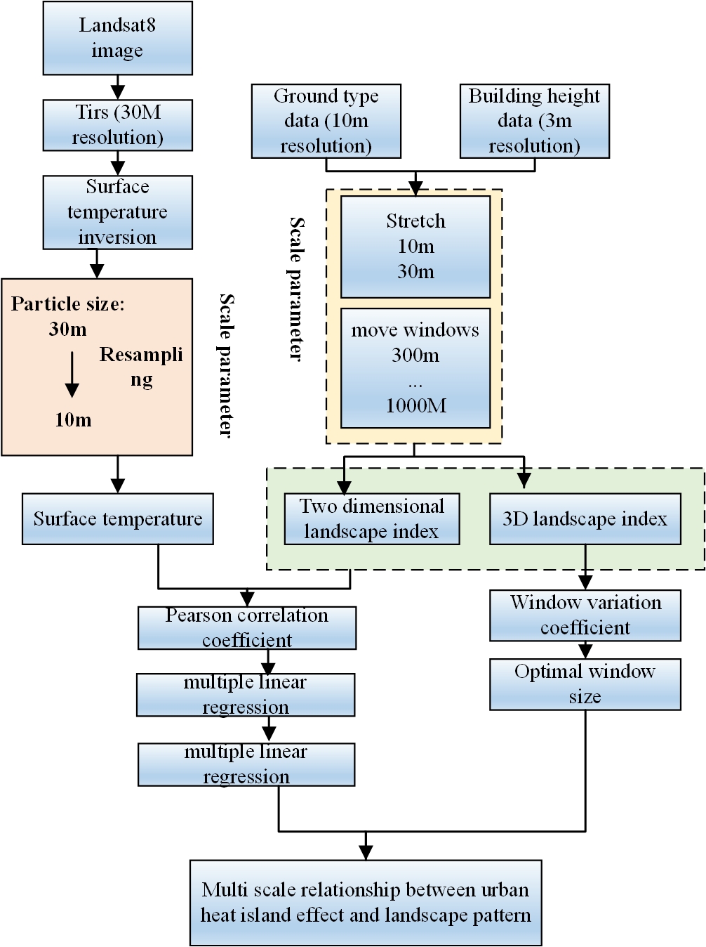
The correlation between landscape indices and art patterns at different scales was analyzed, and the contribution of each landscape index to art patterns in the regression was obtained, and the most important influencing factors of landscape patterns on art patterns were obtained [12]. The main technical route of this research is shown in Figure 1.
To obtain the temporal and spatial information of land use in the complete temporal and spatial sequence before and after dynamic monitoring, and then calculate and analyze the number and distribution characteristics of dynamic land use change samples in different time periods and categories, so as to reflect the temporal and spatial pattern, pattern and mechanism of the evolution of land spatial structure. In different art modes, the land use situation is also different [13,14].
The construction and learning process of the random forest tree is the process of finding the optimal solution for the Gini coefficient measurement criterion, which requires a certain information difference for each sub-sample. The calculation process based on the Gini coefficient is as follows:
\[\label{eq1} \text{Gini} (N) = 1 – \sum\limits_{i = 1}^M {P_i^2} .\tag{1}\]
The training sample set \(N\) is divided into two sub-sample sets, \({N_1}\) and \({N_2}\). The division standard is based on the selection of random feature variables at the judgment node. The number of samples contained in the sample sets \(N,{N_1},{N_2}\) is \(G,{G_1},{G_2}\), The \(G\operatorname{ini}\) coefficient indicator is:
\[\label{eq2} \operatorname{Gini}_{split(k)}(N) = \frac{{{G_1}}}{G}\operatorname{Gini} \left( {{N_1}} \right) + \frac{{{G_2}}}{G}\operatorname{Gini} \left( {{N_2}} \right).\tag{2}\]
Find the minimum value of the \(G\operatorname{ini}\) coefficients as the optimal partition property:
\[\label{eq3} \operatorname{Gini} = \operatorname{Gini} (N) – \operatorname{Gini} {i_{split(n)}}(N).\tag{3}\]
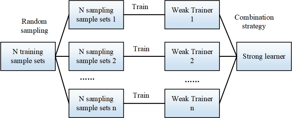
After training \(T\) sample sets to obtain \(T\) weak learners, a combination strategy suitable for solving the classification problem or regression problem is selected. About 1/3 of the sample size, usually called out-of-bag samples, is left after sampling the original dataset. As shown in Figure 2.
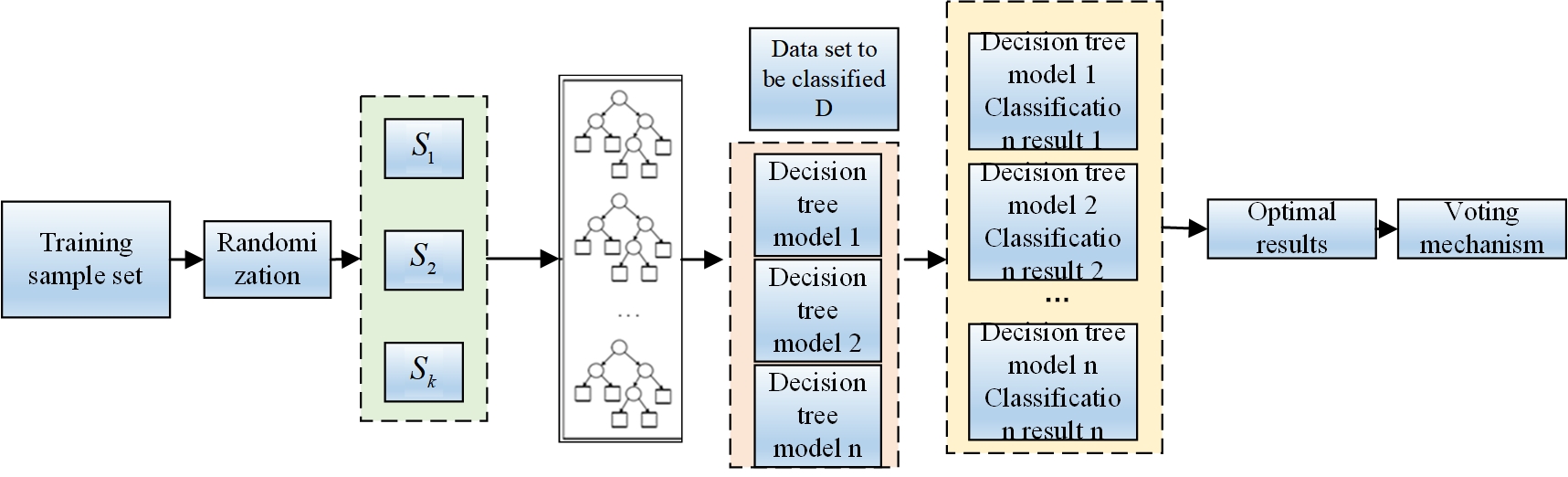
The purpose of selecting the OOB error is to consider that its accuracy verification ability and computational efficiency are optimal relative to the generalization error of the combined classifier estimated by cross-validation [15]. The smaller the value, the higher the accuracy of the model. In addition to model performance evaluation, it is also used to evaluate the importance of feature variables, as shown in Figure 3.
Compared with other machine learning methods such as decision tree, the advantages of random forest are its fast training and prediction speed, high accuracy for classification results, excellent accuracy, and high-dimensional data. It does not require dimensionality reduction during processing and can effectively run-on large data sets; the use of random forest out-of-bag data can evaluate the generalization error, which makes the model generalization ability strong, and can also estimate the importance of feature variables; the whole method realizes simpler and easier to understand.
Landscape index as a measure of landscape characteristics can well describe the shape and distribution characteristics of different patches in the landscape. According to the different description angles of landscape pattern, landscape index can be divided into landscape component index, spatial configuration index and landscape roughness index. In this paper, 15 commonly used two-dimensional and three-dimensional landscape indices are calculated at different scales, among which five are landscape component indices: the largest patch index (LPI) is used to describe the proportion of the largest patches in the landscape, the landscape edge density (ED) It is used to describe the exchange capacity of landscape and external energy [15-17]; 5 kinds of three-dimensional roughness indices: surface root mean square deviation (SQ) is used to describe the landscape plane within the moving window The degree of deviation from the horizontal plane, the surface skewness (SKU) is used to describe the unevenness of the landscape surface relative to the mean elevation plane, the mean height (MEAN) is used to indicate the average height of all cells in the landscape, the maximum height (MAX) is used to represent the maximum height in the landscape, and the sky view factor (SVF) is used to describe the visibility of the sky within the landscape [18]. In this paper, the two-dimensional landscape index is calculated using Frag states 4.2 software, and the three-dimensional landscape index is calculated using a program written by MATLAB software. The calculation formulas and descriptions of all the above landscape indices as shown in Table 1.
| Index name | Calculation formula | Ecological significance |
| Maximum plaque index (%) | $$a_ijA*100$$ | $$a_ij$$ is the two/three-dimensional area of patch, $$A$$ is the total two / three-dimensional area in the window, and IP is the percentage of the maximum patch area in the window in the total window area |
| Edge density (M / HA) | $$\frac{E}{A}{10^6}$$ | $$E$$ is the total boundary length of all patches in the two / three-dimensional landscape, and $$ED$$ is the ratio of the two / three-dimensional boundary length in the window to the total area of the window, which can be used to describe the average area of patches in the window |
| Number of patches | $$ – n$$ | $$BP$$ is the total number of patches in the window |
| Landscape aggregation index | $$\left[ {{\bf{1}} – \frac{{\sum\limits_{j = 1}^n {{p_{ij}}} }}{{\sum\limits_{j = 1}^n {{p_{ij}}} \sqrt {{a_{ij}}} }}} \right]$$ | The cohesion can be used to calculate the aggregation and dispersion of the patches in the window |
| Effective grid area (CHA) | $$\frac{{\sum\limits_{i = 1}^m {\sum\limits_{j = 1}^n {a_{ij}^2} } }}{A}$$ | Positive SH is the ratio of the square sum of all patch areas to the total window area |
As \[\label{eq4} PCC = \frac{{\sum\limits_{i = 1}^N {{x_i}} {y_i}}}{{\sqrt {\sum\limits_{i = 1}^N {x_i^2} \sum\limits_{i = 1}^N {y_i^2} } }},\tag{4}\] when there is no significant correlation between the two, the value approaches 0. Finally, normalize all the obtained values as Eq. (5):
\[\label{eq5} VI{M_j} = \frac{{VI{M_j}}}{{\sum\limits_{i = 1}^c V I{M_i}}}.\tag{5}\]
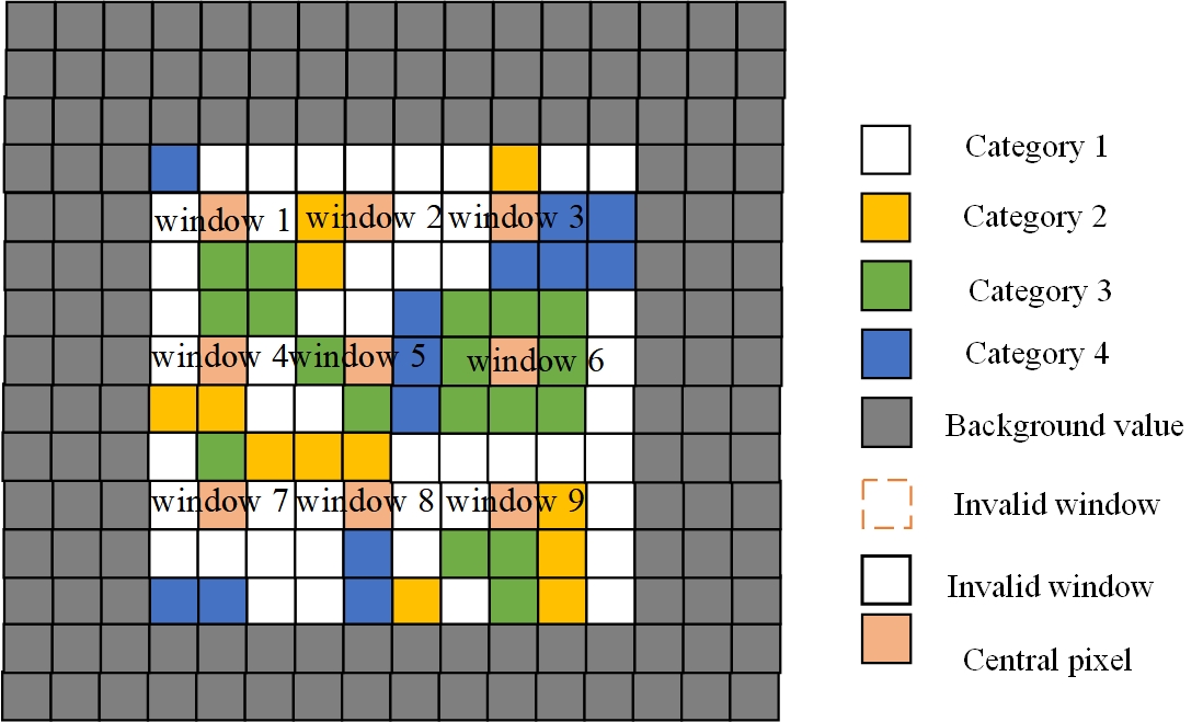
Since the correlation between the calculated indices cannot be completely avoided, overlapping moving windows will make the calculation results of adjacent windows have more serious correlations [18-20], so this experiment uses the non-overlapping moving window method to calculate the study area, as shown in Figure 4.
The research areas are in the rural functional extension area in the center of Beijing and the rural area in Beijing (as shown in Figure 5). Beijing Second Ring Road was completed in September 1992, with a total length of about 32.7 kilometers. It is China’s first fully enclosed and fully interchangeable rural expressway. The inner area of the second ring road is about 62 square kilometers, which is the old city of Beijing. The north-south buildings in the central area of the ring are mainly traditional courtyard houses. The building height is low but the density is high. The inner area of the Fourth Ring Road is about 302 square kilometers. It is a highly built rural landscape with very dense buildings. It is suitable for use as a typical area to study the relationship between rural landscape effects and 3D landscape patterns.
In this paper, Landsat 8 imagery is used to invert the surface landscape, and the spatial resolution of the data is 10M. The dataset is divided into ten ground object categories: cropland, woodland, grassland, shrubs, wetlands, water bodies, permafrost, impervious surfaces, bare land, and ice/snow.
The water body occupies the least proportion in the second and fourth rings, only 3.08% and 1.51%. The impervious surface is the main feature type in the central urban area of Beijing [2], accounting for 76.09% and 76.09% of the total area of the second and fourth rings respectively. The proportion of grassland types in the two study areas is roughly the same, as shown in Table 2.
| Research area | Second ring | Four rings | ||
| Number of pixels (PCs) | Proportion (%) | Number of pixels (PCs) | Proportion (%) | |
| grassland | 488.24 | 7.79 | 211776 | 7.04 |
| Woodland | 81979 | 13.07 | 564784 | 18.75 |
| Water body | 19341 | 3.09 | 564784 | 1.52 |
| Impervious surface | 499982 | 76.10 | 2192024 | 72.74 |
| Building | 149832 | 31.36/23.87 | 647241 | 29.54/21.48 |
| Total | 627833 | 100 | 3014031 | 100 |
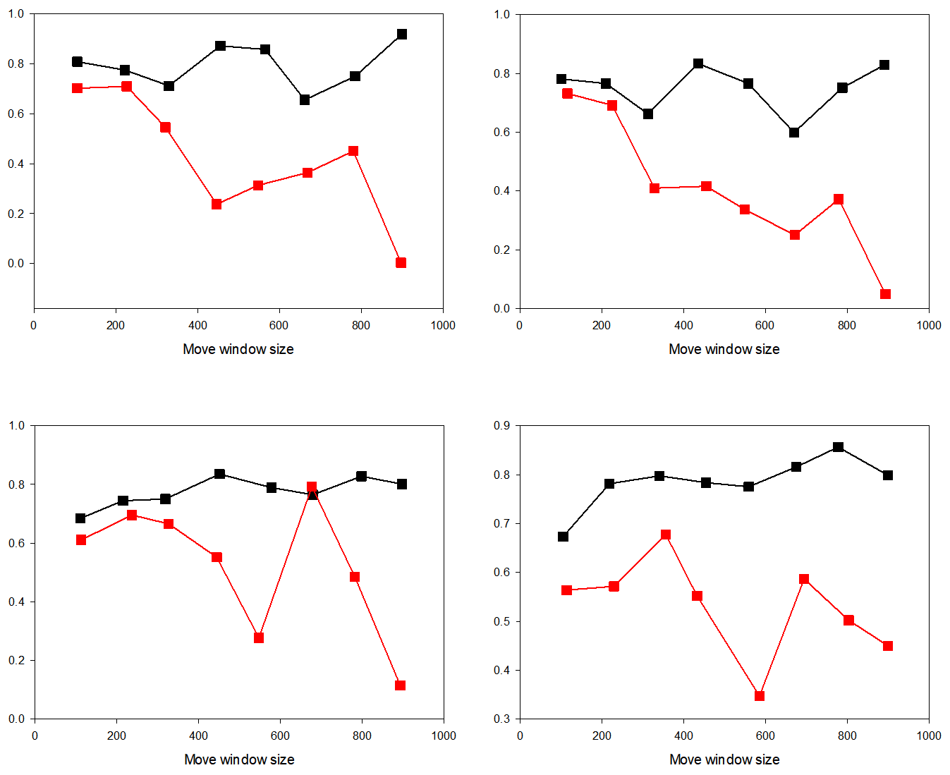
The results of the 10M granularity two- and three-dimensional landscape index and the Pearson correlation coefficient of the art model as shown in Figure 6. All the results meet the significance test with a confidence level of 0.05. The correlation between the three-dimensional landscape index and the art model is generally higher than that of the two-dimensional landscape index. The landscape component index has the second highest correlation with the art model, and the roughness index has the highest correlation with the art model. Mode correlation is the weakest [2,3],
Judging from the degree of influence of various driving factors on construction land in 2015, construction land is mostly distributed in areas with high population density and low altitude. Areas with closer water systems, lower GDP values, and shorter distances from roads are more likely to be distributed; forest land types are more affected by elevation and slope, and are mostly distributed in areas with higher elevations and larger slopes , far away from the railway [5]; waters are most affected by slope and elevation, and least affected by population density and GDP value; other land is most affected by elevation, and factors such as slope, population density and water system have the least impact on the distribution of other land, other land use the distribution range tends to be higher in elevation and closer to the road. The experimental analysis results are shown in Figure 7.
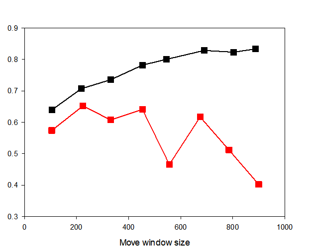
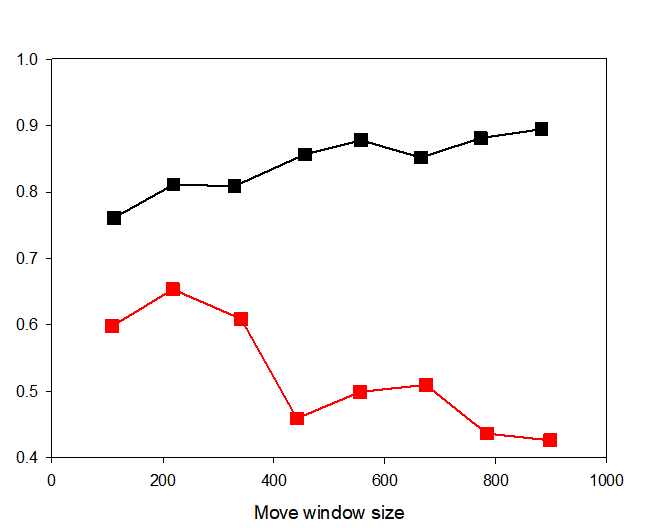
In the regression between the two-dimensional landscape index and the art model, the two-dimensional landscape index itself has a weak interpretation effect on the art model. At the same time, the number of samples calculated in the large window is small, which makes the random forest regression ineffective in learning the data set. Resulting in extremely low regression accuracy for random forest regression when the window size is 1000M. As shown in Figure 8.
It can be seen from Table 3 that the ROC values of the five types of land use in the two periods are all greater than 0.75, which means that the logistic regression model has high precision and can better explain the actual land use spatial distribution in the study area and its relationship with various types of land use.
| Research area | Second ring | Four rings | ||
| Number of pixels (PCs) | Proportion (%) | Number of pixels (PCs) | Proportion (%) | |
| grassland | 488.24 | 7.79 | 211776 | 7.04 |
| Woodland | 81979 | 13.07 | 564784 | 18.75 |
| Water body | 19341 | 3.09 | 564784 | 1.52 |
| Impervious surface | 499982 | 76.10 | 2192024 | 72.74 |
| Building | 149832 | 31.36/23.87 | 647241 | 29.54/21.48 |
| Total | 627833 | 100 | 3014031 | 100 |
This paper uses the random forest regression algorithm to study the multi-scale relationship between the art patterns and the three-dimensional landscape pattern of the urban center in Beijing’s rural areas. The advantage of this study is that the art model is retrieved from remote sensing images, and the art model acquisition at a large spatial scale is realized. In the method, the three-dimensional landscape index is used to replace the traditional two-dimensional index, and the three-dimensional information of the village is introduced to describe the landscape pattern inside the village more accurately. Compared with the general linear regression model, it can eliminate the multicollinearity problem between different landscape indices to a certain extent.
Author declares no conflict of interests.