
Automobiles are gradually becoming automated, networked, and intelligent thanks to the quick advancement of computer and sensor technologies, and autonomous automobiles now have the capacity for perception, decision-making, planning, and control [1]. Although the technology for automatic ambulances is evolving quickly, it still needs testing and refinement. automatic ambulance testing and evaluation are now more crucial than ever. Researchers have been studying the testing and evaluation of unmanned vehicles as of late. For instance, Gipps [2] introduced the rule-based paradigm, and it bases much of its decision-making on necessity, expectation, and safety. [3] selected safe and law-abiding behaviours using a petri net, and created an automatic ambulance real-time decision-making system based on multi-criteria decision-making. One popular technique for rule-based modelling is the finite state machine. The state machine is layered in [4]. The vehicle state is represented by the top layer, driving behaviour is represented by the middle layer, and specific actions and conversion conditions are represented by the bottom layer. An automatic ambulance overtaking decision model is created based on multi-level scenarios in [5,6], where the vehicle driving behaviour is separated into numerous states at various levels based on the hierarchical state machine. Uncertainties in the traffic environment are taken into consideration using statistically based models [7,8]. POMDP and the Bayesian network, which can provide a unified framework for behavioural decision-making for a variety of traffic scenarios [9,10], are among them and the most widely used decision-making models. These testing and assessment techniques need to be modified for settings and traffic scenarios that are more intricate and varied. Real-time needs are growing at the same time because autonomous cars must act swiftly to ensure their own safety and effectiveness.
The transportation environment is full with unknowns, such as the erratic behaviour of other drivers and the state of the weather. Some models in existing methodologies find it difficult to manage this uncertainty efficiently, endangering the accuracy of decision-making. Numerous techniques continue to use manual rule creation and arbitrary assessment. This indicates that the evaluation’s findings may be biassed and vulnerable to individual subjectivity. To further the development of autonomous driving technology and guarantee safety and dependability, the area of automatic ambulance testing and evaluation still needs to overcome these obstacles in order to build more thorough, objective, real-time, and adaptable evaluation techniques.
To this end, researchers [11] created a vehicle evaluation model based on the three factors of task complexity, environmental complexity, and the degree of human intervention, and combined the expandable hierarchical analysis method with the China Intelligent Vehicle Future Challenge’s fuzzy comprehensive evaluation approach to complete the quantitative assessment of the level of intelligence of the unmanned vehicles; researchers [12] evaluated the comprehensive obstacle avoidance system; [13] did a study on the assessment of automatic ambulances’ intelligent behaviour in the setting of curved roads. The complete obstacle avoidance behaviour of unmanned vehicles was evaluated by [14] using the hierarchical analytic approach a study was conducted on the evaluation of the intelligent behaviour of unmanned vehicles in the curved road environment, and the fuzzy comprehensive evaluation approach. Most of the currently used evaluation methods for unmanned vehicles use highly subjective hierarchical analysis, expandable hierarchical analysis, and fuzzy comprehensive evaluation methods, and the majority of these evaluations are focused on a single vehicle intelligence (for example, the intelligent behaviour of unmanned vehicles) or certain specific scenes or vehicle behaviours.
These rule-based models, on the other hand, arrive at decisions by creating rules that are both computationally effective and consistent with driving behaviour. However, rule-based models are vulnerable to the issue of low accuracy since they are influenced by the traits of traffic behaviour, such as uncertainty and discontinuity. Although statistical-based models are more accurate since they account for the traffic environment’s uncertainty [15], they have high computing costs and poor real-time performance.
This work builds a simulation model for path decision-making suitable for dynamic situations by combining the properties of rule-based models and statistical models in order to address the aforementioned issues. Urban environments include more traffic components and a more complex structure than highways. In addition, the majority of the recent studies on lane switching in urban settings use two lanes. The intersection access issue and three-lane lane-changing behaviour of autonomous cars for urban contexts are therefore explored in this study. The following are the main contributions:
Firstly, the paper presents a comprehensive framework for designing automatic ambulance test scenarios, which involves testing in various scenarios with different levels of complexity. The scenarios encompass a wide range of environmental factors, including road conditions, weather and lighting, traffic signals, obstacles, and external interference. By structuring and combining these factors, the test environment can simulate real-world driving conditions effectively, thereby ensuring thorough testing of the automatic ambulance’s capabilities.
Secondly, the paper introduces an evaluation index system for assessing the performance of automatic ambulances. This system comprises three components: determining assessment indices, calculating index weights using the CRITIC and AHP methods, and establishing an evaluation procedure. The evaluation indices cover aspects such as driving security, ride comfort, intelligence, and efficiency, which are essential for evaluating the overall performance of automatic ambulances.
Furthermore, the paper presents methodologies for calculating the weights of evaluation indicators, including both level indicator weights and aggregate indicator layer weights. The CRITIC approach is employed to determine the weights of individual evaluation indicators, taking into account data stability, correlation between indicators, and conflict between indicators. Additionally, the hierarchical analysis method is utilized to calculate the weights of aggregate indicator layers, ensuring a fair and reasonable evaluation of the automatic ambulance’s performance.
Testing in multiple scenarios of varying complexity can be a suitable technique to verify the performance of the driverless car since when a automatic ambulance is travelling on a real road, the road scenario and environment are unknown and complex [16]. The test environment and the test content are both components of the test scenario. The test material need to reflect the actual traffic scenario as closely as feasible. It covers the automatic ambulance’s assessment of its surroundings as well as its capacity for information-based decision-making, planning, and control. Due to the different levels of intelligence of the various automobiles, the test content will be divided into various difficulty levels, and the driving behaviours that the automatic ambulances must exhibit in the test will also be divided into various levels of complexity [17]. According to the driving styles of human drivers, driverless car behaviours can be divided into three categories: basic driving behaviours, advanced driving behaviours, and driving behaviours in complicated surroundings Figure 1.
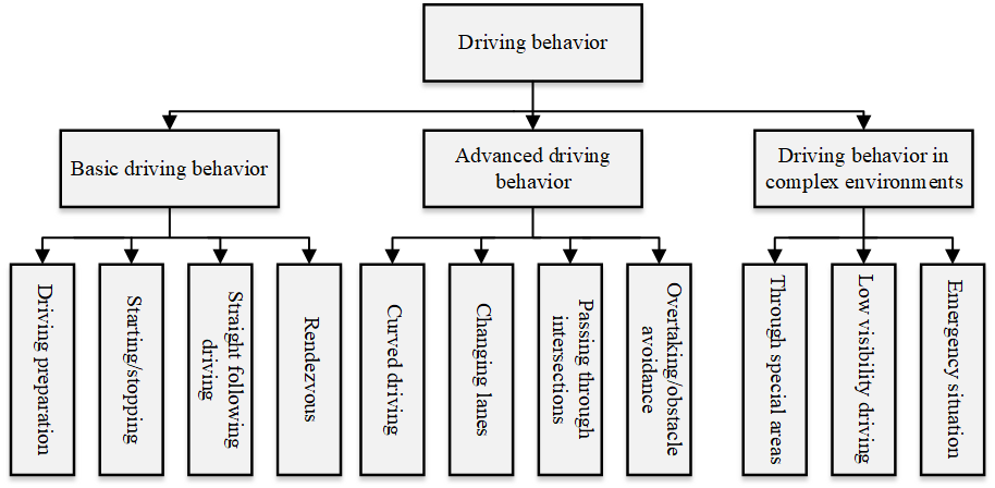
Table 1 lists the many features and parts of the testing environment, including the road environment, weather and illumination environment, traffic signal environment, obstacle environment, and auditory and external interference environment [18]. Different road topology environments can test a driverless car’s ability to recognise lanes; different road surface conditions can test the car’s control; and various traffic signal and obstacle environments can test the car’s ability to perceive its surroundings. Because the driving environment for real vehicles is complex and unpredictable, the testing environment should be as varied as feasible. An environment for testing that is of varying complexity can be built by structuring and combining different environmental factors.
To finish the design of the autonomous car test scenarios, combine test contents with varying levels of complexity and test environments [19].
| Environmental factors | Element composition |
| Road environment | Road surface: sand, asphalt, cementRoad topology: bends, roundabouts, intersections, and ramps Road surface conditions: water accumulation, snow accumulation, and icing |
| Weather and lighting environment | Weather: sunny, rainy, snowy, hailIllumination: direct sunlight at noon, oblique sunlight at dusk, and eveningTraffic signs: speed limit, no left turns, school sections |
| Traffic Signal Environment | Traffic lane routes: single and double solid lines, dashed lines, zebra crossing traffic signal lights |
| Obstacle environment | Static: barricades, fire hydrants, road fencesDynamic: vehicles, pedestrians, non motorized vehicles |
| Auditory environment | Ambulances, fire trucks, police cars |
| External interference environment | Electromagnetic interference, GPS limitation |
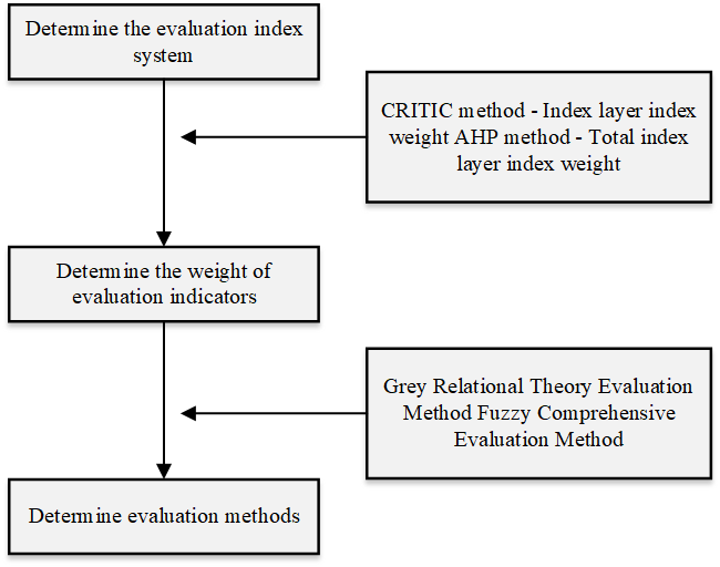
The performance of a driverless car must be assessed following a test in a test scenario [20]. The evaluation system for automatic ambulances includes three components, as shown in Figure 2, which are applied in the CRITIC-based evaluation approach for the grey correlation theory: figuring out the assessment indices for the driverless car, calculating the weights of the indices using the CRITIC and AHP methods, and figuring out the evaluation procedure.
The foundation of unmanned vehicle evaluation is the evaluation index system, and only a fair and reasonable evaluation index system can yield accurate evaluation findings. Therefore, the concepts of comprehensiveness, science, purpose, comparability, and operability should be followed in the creation of the unmanned vehicle assessment index system. The evaluation of unmanned vehicles is finished by assessing how well they performed in the test, in accordance with the phenomenological theory [20].
The CRITIC approach is appropriate for data with a given level of stability and a certain correlation between the studied indicators or components. It is a type of weighting method based on the criterion of the relevance of correlation between strata. The weights of indicators are set using this method, which additionally considers the impact of data volatility and correlation on weights as well as the degree of comparison and conflict between indicators. Given that the mean value has an impact on comparison strength, the coefficient of variation is used in this study instead of the standard deviation of the data to measure comparison strength. Conflict between indicators is based on the correlation between them; if there is a high positive correlation between the two indicators, then there is little conflict between them. The stages for applying the CRITIC technique to determine the weights of indicators are as follows:
Standardisation of Data: The first step involves distinguishing between positive and negative indicators. Assuming there are \(n\) assessment objects and \(m\) evaluation indicators, positive indicators (benefit indicators) are more desirable when larger, whereas negative indicators (cost indicators) are more desirable when smaller. The indicators need to be standardised because their units of measurement vary. The positive indicator is standardised as follows:
\[\label{e1} x_{ij}^\prime = \frac{{x_{ij} – \min \left\{ x_{ij} \right\}}}{{\max \left\{ x_{ij} \right\} – \min \left\{ x_{ij} \right\}}},\tag{1}\]
while the negative indicator is standardised as follows:
\[\label{e2} x_{ij}^\prime = \frac{{\max \left\{ x_{ij} \right\} – x_{ij}}}{{\max \left\{ x_{ij} \right\} – \min \left\{ x_{ij} \right\}}}.\tag{2}\]
Calculation of Contrast Strength: The contrast strength for the \(j\)th indicator is calculated using the coefficient of variation, defined as:
\[\label{e3} V_j = \frac{\sigma_j}{\bar{x}_j}\quad j = 1,2, \cdots ,m,\tag{3}\]
where \(V_j\) is the coefficient of variation, \(\sigma_j\) is the standard deviation of the \(j\)th indicator, and \(\bar{x}_j\) is the mean of the \(j\)th indicator.
Calculation of Correlation Coefficient and Quantitative Conflict: The correlation coefficient between indicators \(i\) and \(j\) is given by:
\[\label{e4} r_{ij} = \frac{\sum\limits_{h = 1}^n \left( x_{hi} – \bar{x}_i \right) \left( x_{hj} – \bar{x}_j \right)}{\sqrt{\sum\limits_{h = 1}^n \left( x_{hi} – \bar{x}_i \right)^2 \sum\limits_{h = 1}^n \left( x_{hj} – \bar{x}_j \right)^2}}\quad i \ne j,\tag{4}\]
where \(x_{hi}\) and \(x_{hj}\) are the values of the \(i\)th and \(j\)th indicators for the \(h\)th object, and \(\bar{x}_i\) and \(\bar{x}_j\) are their mean values.
The conflict between the \(j\)th indicator and other indicators is quantified as follows:
\[\label{e5} \sum\limits_{i = 1}^m \left( 1 – r_{ij} \right) \quad i \ne j.\tag{5}\]
Determination of Indicator Informativeness: The informativeness of each indicator is determined by its degree of contrast and conflict. The informativeness \(C_j\) of the \(j\)th indicator is given by:
\[\label{e6} C_j = V_j \sum\limits_{i = 1}^m \left( 1 – r_{ij} \right) \quad i \ne j \quad j = 1,2, \cdots ,m.\tag{6}\]
Calculation of Indicator Weights: Finally, the weight of each indicator is calculated as follows:
\[\label{e7} w_j = \frac{C_j}{\sum\limits_{k = 1}^m C_k} \quad j = 1,2, \cdots ,m.\tag{7}\]
The relative importance, or weight, of the \(j\)th indicator increases with the value of \(C_j\), indicating that it contains more information and thus has a greater impact on the overall evaluation.
It is challenging to directly quantify the indicators of driving safety, ride comfort, intelligence, and efficiency in the overall index layer, therefore, the weights of the indicators are determined using the hierarchical analysis method.The fundamental tenet of the AHP method is to create a hierarchical structure that describes the functions or characteristics of the system in accordance with the requirements of the problem, and then to compare the relative importance of the factors by comparing them two at a time to create a judgement matrix that ranks the upper factors in relation to the lower factors and provide a ranking of the lower elements’ relative importance in relation to the higher factors. In this study, the relative significance of a vehicle’s function or attribute is assessed using the hierarchical analysis method. In order to evaluate automatic ambulances, this study uses the hierarchical analysis method to rank the relative relevance of four indicators: driving security, comfort, wit, and effectiveness. The steps in applying hierarchical analysis to calculate the weights of indicators are as follows:
| Scale | Definition of importance |
|---|---|
| 1 | Comparison of two equally important factors |
| 3 | When comparing two things, one is somewhat more crucial than the other |
| 5 | When two things are compared, one is more significant than the other |
| 7 | When comparing two things, one is significantly more crucial than the other |
| 9 | When comparing two factors, one is far more significant than the other |
| Indicator Name | Indicator 1 | Indicator 2 | … | Indicator N |
|---|---|---|---|---|
| Indicator | 1 | 1 \({a_{12}}\) | … | \({a_{1n}}\) |
| Indicator2 | \({a_{21}}\) | 1 | … | \({a_{2n}}\) |
| Indicator N | n | \({a_{n1}}\) | \({a_{n2}}\) | 1 |
Create the Evaluation Matrix: Experts are requested to rate the relevance of the \(n\) unmanned vehicle indicators on a scale of 1 to 9 and compare their value two by two using the important definition table in Table 2.
The judgement matrix \(A\) with the diagonal at position 1 is obtained as indicated in Table 3, and the values of the judgement matrix symmetrical about the diagonal elements are inverses of one another.
Calculate the Weights of the Indicators: Solve the maximal eigenvalue and eigenvector of the judgement matrix \(A\) using the sum-product method, normalize it by columns, and then sum the vectors by rows.
\[\label{e8} \overline{a}_{ij} = \frac{a_{ij}}{\sum\limits_{i = 1}^n a_{ij}}.\tag{8}\]
\[\label{e9} w_i = \sum\limits_{i = 1}^n \overline{a}_{ij}.\tag{9}\]
The rows of the judgement matrix averaged to produce the weight vector \(\overline{w}_{ij}\) of \(A\).
\[\label{e10} \overline{w}_{ij} = \frac{w_i}{\sum\limits_{i = 1}^n w_i}.\tag{10}\]
Compute the largest eigenroot of the judgment matrix \(A\):
\[\label{e11} \gamma_{\max} = \sum\limits_{i = 1}^n \frac{\left[ A \overline{w}_i \right]_i}{n \left( \overline{w}_i \right)_i}.\tag{11}\]
Test for Consistency: It is necessary to conduct a consistency test to see whether the weights are reasonable after the judgement matrix’s eigenvectors and maximum eigenvalues have been determined.
\[\label{e12} \text{C.I.} = \frac{\gamma_{\max} – n}{n – 1}.\tag{12}\]
The consistency ratio (C.R.) should meet the condition:
\[\label{e13} \frac{\text{C.I.}}{\text{C.R.}} < 0.1.\tag{13}\]
The judgement matrix is found to have appropriate consistency by Table 4, where C.R. stands for the average random consistency index.
| Indicator n | 3 | 4 | 5 | 6 | 7 |
|---|---|---|---|---|---|
| Average Random Consistency Index C.R. | 0.55 | 0.85 | 1.14 | 1.20 | 1.32 |
| Indicator n | 8 | 9 | 10 | 11 | 12 |
| Average Random Consistency Index C.R. | 1.39 | 1.442 | 1.45 | 1.50 | 1.52 |
Both qualitative and quantitative evaluation techniques are used in the evaluation of unmanned vehicles. By monitoring the behaviour or condition of the evaluated object, qualitative evaluation methods, like inductive analysis, analyse unmanned vehicles using non-quantitative approaches and drawing on the knowledge, experience, and judgement of experts. Quantitative evaluation techniques gather data using mathematical techniques, process it, and then present a numerical summary of all evaluation-related information. Grey correlation analysis, approximate ideal solution sequencing, fuzzy comprehensive evaluation, back propagation neural network, and weighted arithmetic average are some commonly used quantitative evaluation techniques. In this study, two quantitative assessment methods are used to evaluate unmanned vehicles: the fuzzy comprehensive evaluation method and the grey correlation theory evaluation method.
The term “grey system” describes a system that humans are unable to fully understand through information. Grey system theory is a theory that primarily examines and deals with complex systems from the viewpoint of incomplete information. Rather than analysing the system from its internal special law, it realises the understanding of the internal trend of changes and interrelationships at a higher level through continuous mathematical processing of information at a certain level of the system.
Because the assessment indices are too complex to list and analyse one at a time, the evaluation of unmanned vehicles might be conceived of as a grey system, the grey correlation theoretical analysis approach is taken into consideration. The goal of grey correlation analysis is to analyse changes in the development trend of things without imposing strict limits on sample size or taking into account in advance whether the data distribution follows a typical distribution pattern. The calculation required is also relatively small. Grey correlation analysis’ fundamental goal is to determine the degree of geometrical similarity between two curves in order to determine whether they are closely connected. The correlation between the respective series is stronger and smaller the closer the curves are to one another. Grey correlation theory decreases the impact of subjective elements and promotes the objectivity of evaluation findings by measuring a vehicle’s performance in terms of the correlation between the actual value and the indicator’s optimal value. The performance of the vehicle improves as the correlation increases. The following are the steps of the grey correlation theory evaluation method:
To create the matrix that will be evaluated, decide on the evaluation indexes and arrange the index values. The vehicle successfully completes the test in m test situations, and after creating the assessment matrix by analysing the test data \({\left( {{C_{ij}}} \right)_{m \times n}}\), \({C_{ij}}\) in the ith test scenario, n evaluation index values are acquired for the value of the jth index.
Identify the reference sequence \({C_{0}}\), which consists of each indicator’s ideal values. In general, the greatest value of the indicator under various test scenarios is the ideal value for positive indicators, while the minimum value of the indicator under various test scenarios is the optimal value for negative indications; the optimal value for indicators with critical values is the critical value of the indicator; and for indicators that are difficult to distinguish between positivity and negativity, experts will be invited to determine the optimal value of the indicator.
Values from evaluation indicator are processed without dimensions. The mean value method is used to process indicator values without regard for dimensions.
\[\label{e14} {X_i}(j) = \frac{{{C_i}(j)}}{{{C_j}}}\quad i = 1,2, \cdots ,m.\tag{14}\]
\[\label{e15} {C_j} = \frac{1}{{m + 1}}\sum\limits_{i = 0}^m {{C_i}} (j)\quad j = 1,2, \cdots ,n.\tag{15}\]
Determine the index scores and correlation coefficients between the comparative and reference series.
\[\label{e16} {\xi _i}(j) = \frac{{{{\min }_i}{{\min }_j}\left| {{X_0}(j) – {X_i}(j)} \right| + \rho {{\max }_i}{{\max }_j}\left| {{X_0}(j) – {X_i}(j)} \right|}}{{\left| {{X_0}(j) – {X_i}(j)} \right| + \rho {{\max }_i}{{\max }_j}\left| {{X_0}(j) – {X_i}(j)} \right|}}.\tag{16}\]
In the equation, the resolution coefficient, denoted by the number \(\rho\), is typically between 0.1 and 0.5, and the correlation coefficients for the jth metric in the ith test scene are denoted by the numbers \({\left( {{\xi _{ij}}} \right)_{m \times n}}\) and \({\xi _{ij}}\) in the matrix of correlation coefficients. Averaging the scores of the same indicator in various test scenarios will yield the indicator’s score, presuming that the weights of the various test scenarios are the same.
\[\label{e17} {s_j} = \frac{1}{m}\sum\limits_{i = 1}^m {{\xi _i}} (j).\tag{17}\]
Calculate the total indicator score (grey correlation). To get the indicator scores corresponding to the entire indicator layer, multiply the indicator scores by the indicator weights.
\[\label{e18} {\gamma _h} = \sum {{s_j}} {w_j}\quad h = 1,2,3,4.\tag{18}\]
The total indicator weights and total indicator scores are then combined to get a composite score for the vehicle.
The fuzzy comprehensive assessment method transforms qualitative evaluation into quantitative evaluation, in accordance with the fuzzy mathematics attachment degree theory. This approach works well for managing fuzzy, difficult-to-quantify problems and non-deterministic problems, but it depends on experts to assess the indexes, which is very subjective. But the fuzzy comprehensive evaluation technique, which depends on professionals scoring the indicators, heavily weighs subjective aspects. Because it includes three levels and uncertainty, the fuzzy comprehensive evaluation approach is suitable for evaluating unmanned vehicles using the aforementioned evaluation index system. The steps of the fuzzy comprehensive assessment approach are as follows:
Identify Evaluation Indicator Sets for Automatic Ambulances:
\[\label{e19} U = \left\{ u_1, u_2, \cdots , u_i, \cdots , u_n \right\},\tag{19}\]
where \(u_i\) is the evaluation index for automatic ambulances and \(n\) is the total number of independently varying elements.
Determine the Automatic Ambulance Evaluation Set:
\[\label{e20} V = \left\{ v_1, v_2, \cdots , v_j, \cdots , v_m \right\}.\tag{20}\]
The evaluation set represents the range of values for the indicator’s evaluation result, and \(v_j\) is the evaluation result of the autonomous car in the \(j\)-th evaluation set.
Determine the Evaluation Matrix of the Indicators \(R\):
\[\label{e21} \mathbf{R} = \left( \mathbf{R}_1, \mathbf{R}_2, \cdots , \mathbf{R}_n \right) = \left( r_{ij} \right)_{n \times m}.\tag{21}\]
The degree of connection between the evaluation index \(u_i\) and the evaluation level is indicated in the calculation by \(R\)’s \(j\)-th column and \(i\)-th row. By comparing \(n\) evaluation indexes, we determine the \(n\)-th row and \(m\)-th column of the affiliation evaluation matrix \(R\).
Choose the Single-Level Fuzzy Comprehensive Assessment Model: Combine the weights of the evaluation indicators with the affiliation evaluation matrix to obtain the single-level fuzzy complete assessment results for the evaluation indicators.
\[\label{e22} B = WR = \left( b_1, b_2, \cdots , b_m \right),\tag{22}\]
where \(b_j = \sum\limits_{i = 1}^n w_i r_{ij}\) for \(j = 1, 2, \cdots , m\).
Comprehensive Fuzzy Multi-Level Evaluation Model: The automatic ambulance’s fuzzy comprehensive evaluation findings are derived by combining the weights of the indicators with the findings of the single-level fuzzy comprehensive evaluation in the complete indicator layer.
\[\label{e23} M = WB.\tag{23}\]
Determine the Overall Evaluation Score: The fuzzy affiliation degree of the assessment set is separated into five levels (excellent, good, average, poor, very poor), which are assigned to \(\mu = (1.0, 0.8, 0.6, 0.4, 0.2)\). The overall score formula is as follows, in accordance with the principle that higher vehicle scores are better.
\[\label{e24} C = M \mu \times 100.\tag{24}\]
The dynamic path algorithm and proposed traffic state machine model, which revolve around the intelligent driving decision-making system, are implemented in this work. The Unity3D engine is used to realise the outcomes of several decision-making simulation scenarios in order to test the efficacy and efficiency of the algorithm. Finally, the performance analysis of the method described in this paper is completed. A vehicle length of 4.5 metres, a vehicle width of 2 metres, and a lateral displacement time of 2 seconds are all used in the experiment on a three-lane road with a length of 300 metres.
These three phases make up the simulation of an unmanned decision-making system:
Based on the intelligent vehicle’s environment sensing layer and path planning layer in the awareness region, detecting arbitrary conditions for acting;
The dynamic goal route algorithm determines the risk factor that could arise from the issuance of an action in a dynamic environment in the conflict region;
Based on the traffic state machine and the danger factor, the decision-making system decides what to do and starts taking action.
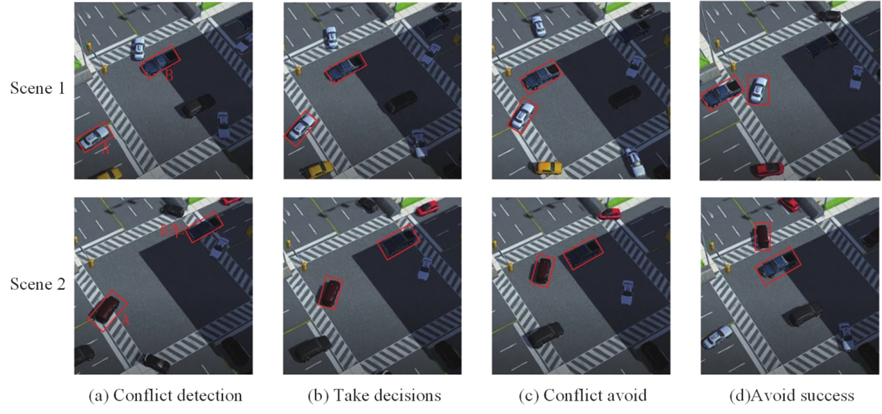
avoiding conflicts at intersections. By focusing on the state transformation of vehicles A and B based on the traffic state machine and the dynamic target route algorithm, this experiment mimics the problem of conflict avoidance in the conflict region of an intersection.Vehicles A and B are expected to be able to determine the physical state of other vehicles for conflict detection once they enter the awareness region, as shown in Figure 3. The experiment is split into two situations based on the assumption that there may be a disagreement between cars A and B.
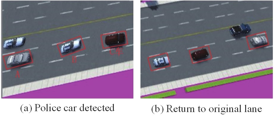
Lane shift in an emergency. Simulate the procedure of lane-changing for cars in an emergency. Vehicle A in Figure 4 is a police car, and vehicles B and C are self-driving cars. The action state and trajectory of the police car are pre-specified by the system once it reaches the awareness region of cars B and C in the incident.
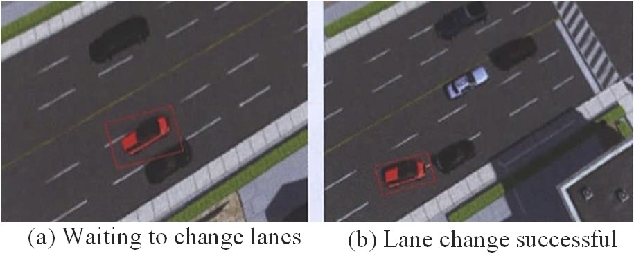
Forced Lane Change Experiment. Play out the process of a car changing lanes to get to its destination. The path planning layer provides a left turn command at the following intersection to the red autonomous car, as seen in Figure 5, so that it can go to its destination.
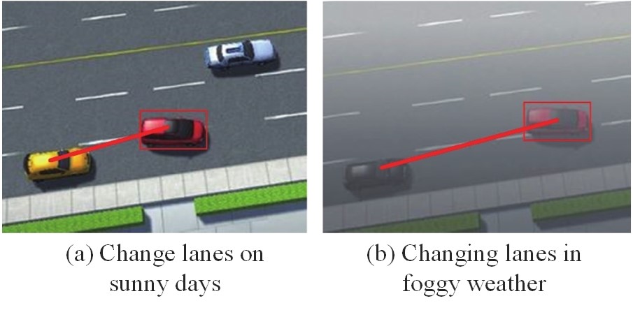
Automatic Lane Change. Simulated scenarios involved automobiles changing lanes to increase speed. Simulated lane-changing situations included both clear and foggy days. In the sunny day scenario, the inner, middle, and outer lanes’ average speeds were set to 50 km/h, 60 km/h, and 70 km/h, respectively, while the equivalent foggy day scenario’s average speeds were set to 30 km/h, 40 km/h, and 50 km/h. At the start of the experiment, it was presummated that the automatic ambulances complied with the arbitrary lane-changing requirements.
On a sunny day, Table 5 depicts the speed of the automated vehicle during the lane-changing procedure. With a decision delay of 0. 6 seconds, the automatic ambulance begins changing lanes in 0. 6 seconds and completes the process in 3. 6 seconds. The speed increases from 60 km/h before changing lanes to 70 km/h after changing lanes. On a hazy day, the autonomous car begins changing lanes in 2 seconds and completes the shift in 5. 5 seconds, with a decision delay of 0.82 seconds. Taking into account the consequences of foggy days The speed is increased to 45 km/h based on the full-speed difference continuous following model, and driving for a specific distance in order to increase the distance from the rear vehicle in the target lane, taking into account the effect of foggy weather, in order to avoid rear-end collision with the target vehicle. The experimental simulation situations in bright and foggy days are depicted in Figure 6, when changing lanes in a foggy environment, the entry point of the automatic ambulance’s red car is further distant from the target lane’s rear car.
| – | Clear day | Foggy days |
|---|---|---|
| Initial speed/(km/h) | 60 | 40 |
| Speed during lane change/(km/h) | 60 | 45 |
| Speed after lane change/(km/h) | 80 | 50 |
| Lane change time/s | 0.6 | 2 |
| Distance between lane change and target rear vehicle/m | 6.2 | 11.1 |
Unmanned decision-making systems use real-time as a key performance indicator, and various programme iteration intervals are specified to determine the amount of time needed to assess the risk factor (Table 6). The programme will presume that the surrounding vehicles maintain a constant speed during the evaluation process. The longer the iteration interval, the longer the evaluation process will assume that the surrounding vehicles are moving at a constant speed. This will make the surrounding vehicles less sensitive to changes in driving conditions, which will decrease the accuracy of the risk coefficient evaluation. The influence of a change in the vehicle’s speed on accuracy, however, is minimal when the time interval is set to 0.1s, and the assessment time of 0.098s can meet the criterion that the planning time of the automatic ambulance be less than 200ms.
| Iteration interval | 0.1 | 0.2 | 0.3 | 0.4 | 0.5 |
|---|---|---|---|---|---|
| Evaluation time | 0.095 | 0.70 | 0.050 | 0.048 | 0.046 |
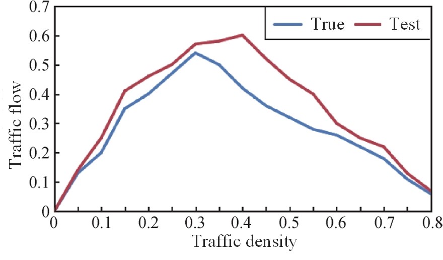
As illustrated in Figure 7, variations in traffic flow under various vehicle densities are examined in order to better validate the improvement in driving efficiency achieved by the strategy described in this paper. The studies demonstrate that the simulation’s saturation flow rate is 0. 6, higher than the measurement’s 0.54, and that the simulation’s saturation traffic density is higher than the measured data’s. Road section findings for the inside, outside, and in the three lanes of the lane change rate during peak and non-peak periods are provided in Table 6, along with experimental simulation results for comparison. It is clear that this paper’s simulation contributes to an improvement in the rate of lane changes, particularly during peak hours when traffic density is higher and the benefits of this paper’s approach are more apparent.
| – | – | The inside lane | Middle lane | The outside lane |
|---|---|---|---|---|
| Peak period | Actual measurement results | 4.5 | 7.8 | 14.2 |
| Peak period | Simulation result | 7.0 | 13.25 | 20.52 |
| Ordinary period | Actual measurement results | 7.5 | 12.6 | 20.71 |
| Ordinary period | Simulation result | 2.1 | 15.12 | 22.06 |
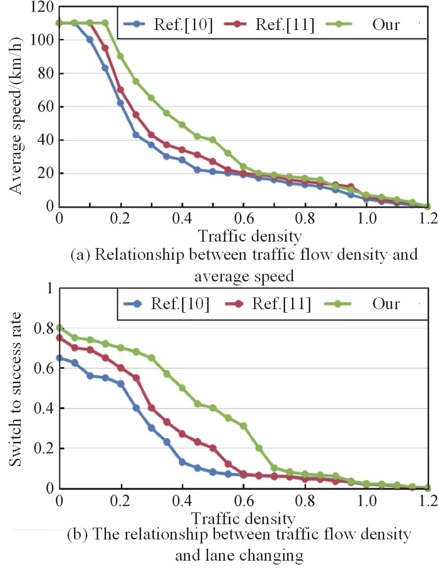
Models from literature [10] and literature [11] are contrasted to those in this essay. The impact of increasing traffic density \({\rho _0}\) on the three models’ average speeds is seen in Figure 8. There is now little interaction between the cars, a huge distance between them, and little impact from the three models on the average speed. The behaviour of changing lanes will have the effect of slowing down traffic behind both the original lane and the target lane as traffic congestion rises.
The comparison shows that the average speeds of the models in this study can rise by up to 32 km/h and 22 km/h . The behaviour of changing lanes has less of an effect on traffic flow when the congestion factor is greater. The success rates of the three models fluctuate when traffic density rises. When the density is low, there is not much of a difference between the three models, but as the density increases, the method described in this work can boost the success rate of lane change by up to 37% and 25%, respectively, in comparison to the other two models.
According to experts’ estimations, the ideal straight-lane yielding distance is 35 metres, and the ideal yielding speed is 10 metres per second. These values are included in the driving safety indices for the comprehensive straight-lane yielding scenario. There is a comfort threshold in the indexes of y-direction acceleration peak and transverse angular velocity peak, thus the best values of these indexes are 0.12g for the y-direction acceleration peak and 15 rad/s for the transverse angular velocity peak. According to the various positivity and negativity of the indexes, the highest and smallest values in the test data are the best values for other indices. Therefore, 0.12 g is the ideal peak y-direction acceleration, and 15 rad/s is the ideal peak traverse angular velocity. According to the various positivity and negativity of the indexes, the highest and smallest values in the test data are the best values for the other indices. The scores of each index and the overall score of the vehicle are determined using the evaluation model based on grey correlation theory, as shown in Table 8.
For quantitative evaluation, a fuzzy comprehensive evaluation method is applied. Invite 80 senior drivers and 20 specialists in the field of autonomous and intelligent vehicles to rate the indicators in accordance with the scoring criteria. Table 9 and 10 illustrate the scoring criteria and a portion of the experts’ rating tables.
| Vehicle comprehensive score | Overall indicators | Total Index Score | Index | Indicator score |
| – | – | – | Avoiding a safe distance | 65 |
| 76.5 | Ride comfort | 56 | Standard deviation of vehicle speed | 95 |
| – | Intelligence | 85 | Maximum value of vehicle offset center to center distance | 75 |
| – | Efficiency | 90 | Task completion time | 85 |
| Good | Preferably | Same as | Range | Differ from |
|---|---|---|---|---|
| 9 | 8 | 5 | 3 | 1 |
| Index | 1 | 2 | 3 | 4 | 5 | 6 | 7 | 8 | 9 | 10 |
| Vehicle speed during avoidance | 8 | 6 | 6 | 6 | 6 | 5 | 8 | 8 | 6 | 6 |
| Avoiding a safe distance | 8 | 8 | 9 | 5 | 8 | 8 | 7 | 5 | 7 | 5 |
| lane keeping | 9 | 7 | 8 | 7 | 5 | 6 | 6 | 5 | 8 | 7 |
| Standard deviation of vehicle speed | 7 | 9 | 8 | 5 | 7 | 8 | 5 | 9 | 7 | 7 |
| Peak acceleration in x-direction | 7 | 7 | 8 | 9 | 7 | 8 | 7 | 8 | 8 | 9 |
| Peak acceleration in Y-direction | 5 | 2 | 7 | 1 | 1 | 4 | 5 | 6 | 5 | 5 |
| Maximum value of vehicle offset center to center distance | 7 | 8 | 7 | 7 | 9 | 9 | 7 | 5 | 8 | 9 |
| Distance when sensing obstacles | 6 | 7 | 9 | 7 | 7 | 7 | 5 | 5 | 7 | 8 |
| Task completion time | 7 | 8 | 8 | 7 | 7 | 5 | 7 | 5 | 5 | 7 |
| Average speed | 7 | 7 | 7 | 7 | 5 | 5 | 8 | 5 | 7 | 7 |
The affiliation matrix is derived from the expert rating scale in the fuzzy comprehensive assessment method, and the scores of the indicators in the total indicator layer and the comprehensive score of the vehicle are calculated by adding the weights of the indicators. Table 11 displays the computation outcomes for the fuzzy comprehensive evaluation method and the grey correlation evaluation method.
| Index | Method for evaluating grey correlation | Method for a fuzzy, comprehensive evaluation |
|---|---|---|
| Ride comfort | 55 | 65 |
| Intelligence | 80 | 85 |
| Efficiency | 90 | 78 |
| Driving safety | 86 | 81 |
| Vehicle comprehensive score | 78.5 | 78 |
The peak angular velocity and x-peak acceleration of the pendulum are much above the threshold of comfort, according to the calculation findings, indicating that the riding comfort of the vehicle during avoidance needs to be improved. The standards for comfort are met by the minimal standard deviation of the vehicle’s speed and its peak acceleration in the x-direction.The maximum value of the vehicle offset centre distance when the vehicle is travelling steadily on a straight road is very small, indicating that the vehicle can correctly identify the lane lines; the vehicle can detect pedestrians, non-motorized vehicles, and motor vehicles in advance and take evasive action before the collision; additionally, it can finish the evasive move in a brief amount of time. The optimal values of the intelligence and efficiency indicators are taken from the test data in the evaluation of ride comfort, intelligence, and efficiency that uses the grey correlation theory evaluation method, whereas the expert assessments, which have a strong subjective influence, determine the scores of the indicators in the fuzzy comprehensive evaluation technique.
In terms of driving safety, it can be seen that the automatic ambulance did not collide during the test, could accurately drive along the lane line and keep the lane well, could correctly identify the obstacles and successfully avoid them, and the avoidance safety distance, though larger than the optimal value provided by the test, was still within acceptable limits. However, driving too fast while avoiding something will compromise the car’s ability to go safely. When evaluating driving safety using the grey correlation theory evaluation method, only the optimal values of the two indicators—safe distance and speed—are determined by the experts. In contrast, the expert-scored indications used in the fuzzy comprehensive evaluation approach yield ratings that are somewhat different from the results of the subjective evaluation.
Although the scores of the indicators in the overall indicator layer differ greatly between the two evaluation methods, the assessment results are extremely consistent when compared to the fuzzy comprehensive evaluation method and grey correlation theory. The scores of the comfort and efficiency indicators in the fuzzy comprehensive evaluation method differ slightly from those in the grey correlation theory evaluation method because of the high subjectivity of experts in the process of scoring and determining the degree of affiliation of the indicators. The reference sequence of the grey correlation theory evaluation method contains the optimal values, and the optimal values of the majority of the indexes are determined by the experimental data, with a small portion being provided by experts. This effectively reduces both the use of the algorithms directly and the impact of human subjectivity on the review process. This technology can significantly lower the cost of testing and evaluating unmanned vehicles by businesses in real-world applications because it does not necessitate the involvement of a huge number of experts.
This study builds a vehicle evaluation index system, completes the design of the unmanned vehicle test scenario from the viewpoints of test content and test environment, and evaluates unmanned vehicles using the grey correlation theory evaluation technique based on the CRITIC method. This method reduces the subjectivity of the evaluation index weight in two ways: on the one hand, it uses the reference sequence in the grey correlation theory evaluation model in addition to the CRITIC objective weighting method to determine the index weight of the evaluation index layer and the AHP method to determine the index weight of the total index layer. The grey correlation analysis method’s objective description of the underlying indicators is used to identify the ideal value. Both the quantitative evaluation findings of automatic ambulances and the method’s quantitative analysis of evaluation indicators at all levels are improved by the combination of the two.providing a trustworthy benchmark for future advancements in driverless technologies.