Further Results on Radio Number of Wedge sum of Graphs

1. Introduction

Radio labeling of graphs is originated from frequency assignment problem for radio transmitters [1]. The problem is to assign distinct frequencies to radio transmitters while avoiding interference between transmitters that are geographically close to each other. Moreover, it is desired to minimize the frequency bandwidth. The situation is modeled by using graph theory as follows: radio transmitters are represented by vertices of a graph and two vertices are adjacent if their corresponding transmitters are geographically close enough to produce interference. The positive integers are assigned to vertices of the graph subject to a restriction concerning the distances between them; the goal is to minimize the largest integer used. For a simple connected graph \(G\) with vertex set \(V\), let \(d(x,y)\) denote the distance between vertices \(x\) and \(y\). Let \(\epsilon(x)\) denote the eccentricity of the vertex \(x\), i.e., the maximum possible distance from the vertex \(x\) to any vertex of the graph \(G\). Let \(diam(G)\) denote the diameter of \(G\), which is the maximum possible distance between any pair of vertices in \(G\) (i.e., the maximum eccentricity in \(G\)). A radio labeling (or multilevel distance labeling) for \(G\) is an injective function \(c: V\rightarrow \{1,2,3,\ldots\}\) satisfying for each pair of distinct vertices \(x\) and \(y\). The above condition is called the radio condition. The largest number in the range of \(c\) is called the span of the labeling \(c\), denoted by \(span(c)\). The radio number of \(G\), denoted by \(rn(G)\), is the minimum span taken over all radio labelings of \(G\), i.e., \[rn(G):=\min \ \{span(c) \ : \ c \mbox{ is a radio labeling of } G\}.\] Radio labeling for a number of graph families has been studied since its introduction in 2001 by G. Chartrand et al. [2]. Following are few recent references: [3,4,5,6,7,8,9,10]. For a comprehensive and updated survey, the reader is referred to [11]. Throughout the paper, all our graphs are simple and connected. We use \(V(H)\) for the vertex set of a graph \(H\).

Definition 1. Let \(H\) be any graph. For a fixed \(z\in V(H)\), the level structure w.r.t. \(z\) is defined to be a partition of \(V(H)\) into subsets \[L_i(z,H):=\{v\in V(H) \ : \ d(z,v)=i\}\] called levels. In this case, vertex \(z\) is called a root vertex of \(H\).

Definition 2. For a fixed root \(z\in V(G)\), the mapping defined by \[l(v):=d(z,v)\] on \(V(G)\) is called the level function w.r.t. \(z\).

Definition 3. We say that a graph \(H\) has level tuple \((l_1,l_2,\ldots,l_r)\in N^r\) at \(z\), if \(l_i=|L_i(z,H)|\).

Definition 4. Let \(H_1, H_2, \ldots,H_{k\geq2}\) be graphs with level tuple \((l_1,l_2,\ldots,l_r)\) at \(z\in V(H_t)\) for all \(t\). Then \(J^k(l_1,l_2,\ldots,l_r)\) is defined to be the graph \(\cup_{t=1}^k H_t\), where \(H_t\cap H_{t’}=\{z\}\) for \(t\not=t’\). In other words, \(J^k(l_1,l_2,\ldots,l_r)\) is the wedge sum of \(H_t\).

Definition 5. Let \(H\) and \(H’\) be two graphs of same order with level tuples \((l_1,l_2,\ldots,l_r)\) and \((l’_1,l’_2,\ldots,l’_r)\) respectively, at \(z\in H\cap H’\). Then \(J\left(\frac{l_1}{l’_1},\frac{l_2}{l’_2},\ldots,\frac{l_r}{l’_r}\right)\) is defined to be the wedge sum of \(H\) and \(H’\).

In [10], authors compute the radio number of \(J^k(l_1,l_2,\ldots,l_r)\) for \(k\geq2\), by imposing the following condition on the tuple \((l_1,l_2,\ldots,l_r)\): In this paper, we compute the radio number for a significantly larger class of \(J^k(l_1,l_2,\ldots,l_r)\) by relaxing the above condition on \((l_1,l_2,\ldots,l_r)\). Moreover, we determine the radio number for some classes of \(J(\frac{l_1}{l’_1},\frac{l_2}{l’_2},\ldots,\frac{l_r}{l’_r})\). The definition of \(J^k(l_1,l_2,\ldots,l_r)\) and \(J\left(\frac{l_1}{l’_1},\frac{l_2}{l’_2},\ldots,\frac{l_r}{l’_r}\right)\) allows to compute the radio number for a large class of graphs.

Throughout the paper, we use the following settings for \(J^k(l_1,l_2,\ldots,l_r)\) and \(J\left(\frac{l_1}{l’_1},\frac{l_2}{l’_2},\ldots,\frac{l_r}{l’_r}\right)\): \(n\) be the number of vertices, \(d\) be the diameter and \(z\) be the identified vertex given in Definitions 4 and 5. Note that \(d=2r\) for both graph families. We take \(r\geq2\). Let \(l\) be the level function w.r.t. \(z\) and \(H_1,H_2,\ldots,H_k,H,H’\) be graphs mentioned in the construction of \(J^k(l_1,l_2,\ldots,l_r)\) and \(J\left(\frac{l_1}{l’_1},\frac{l_2}{l’_2},\ldots,\frac{l_r}{l’_r}\right)\). In all expressions with summation, we use the convention that \[\sum_{s=a}^b A_s=A_a+A_{a+1}\cdots+A_b=0 \mbox{ for } a>b.\]

2. Radio number of \(J^k(l_1,l_2,\ldots,l_r)\)

In this section, we compute the radio number of \(J^k(l_1,l_2,\ldots,l_r)\) when For convenience, we set \[\theta:=\left\lfloor\frac{r+1}{2}\right\rfloor.\] To establish our result, we use the following lemma proved in [10].

Lemma 1. Let \(G=J^k(l_1,l_2,\ldots,l_r)\) and let \(z=x_0\), \(x_1,\ldots,x_{n-1}\) be an ordering of \(V(G)\) such that for \(p>0\),

1. \(x_p\in H_t\) whenever \(p\equiv t \ ({\rm mod} \ k)\), and
2. \(l(x_{p})+l(x_{p+1})\leq r+1\).

Then \(c(x_p)=1+p(d+1)+l(x_p)-2\sum_{s=1}^{p}l(x_s), \ 0\leq p\leq n-1\) is a radio labeling. Moreover, if \(l(x_{n-1})=1\) then \(c\) is optimal and \[rn(G)=c(x_{n-1})=2+(n-1)(d+1)-2k\left[\sum_{s=1}^{r} sl_s\right].\]

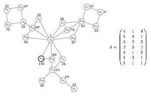
We provide an ordering of the vertices of \(J^k(l_1,l_2,\ldots,l_r)\) represented by \(x_0,x_1,\ldots,x_{n-1}\), which satisfies the conditions of Lemma 1. We represent the desired ordering by the following matrix: \[A=\left(\begin{array}{cccc} l(x_1) \ \ & l(x_2) & \cdots & \ l(x_k)\\ l(x_{k+1}) \ \ & l(x_{k+2}) & \cdots & l(x_{2k})\\ \vdots & \vdots & \cdots & \vdots\\ l(x_{n-k}) \ \ & l(x_{n-k+1}) & \cdots & l(x_{n-1}) \end{array}\right).\] The entry \(a_{j,t}=l(x_p)=i\) of the above matrix corresponds to \(j\)-th vertex of \(L_i(z,H_t)\). Note that the vertices of \(L_i(z,H_t)\) can be ordered arbitrarily. To obtain the desired ordering, we need to construct a matrix whose each column consists of the following entries \[\underbrace{r,r,\ldots,r}_{l_r-times}, \ \underbrace{r-1,r-1,\ldots,r-1}_{l_{r-1}-times}, \ \ldots, \ \underbrace{2,2,\ldots,2}_{l_2-times}, \ \underbrace{1,1,\ldots,1}_{l_1-times}\] placed in some order such that \(l(x_i)+l(x_{i+1})\leq r+1\) and \(l(x_{n-1})=1\). This means that the consecutive entries of \(r\) must be \(1\), the consecutive entries of \(r-1\) must be 1 or 2 and so on. In order to present our desired matrices conveniently, we define a couple of parameters using \((l_1,l_2,\ldots,l_r)\). For \(i=\theta+1,\theta+2, \ldots,r\) and for each \(m=1,2,\ldots,r+1-i\), we define: The values \(\eta(i,m)\) can be determined recursively in the following order: \[\eta(r,1),\] \[\eta(r-1,2), \ \eta(r-1,1),\] \[\eta(r-2,3), \ \eta(r-2,2), \ \eta(r-2,1),\] \[\vdots\] \[\eta(\theta+1,r-\theta), \ \eta(\theta+1,r-\theta-1), \ \ldots, \ \eta(\theta+1,1).\] Moreover, observe that \(\eta(i,m)\) is defined in such a way that for each \(i\), one gets \(\sum_{m=1}^{r+1-i}\eta(i,m)=l_i\). Next for \(i=1,2,\ldots,\theta\), we define: Now we give the mentioned matrices. There are two cases depending on the parity of \(k\).

Case 1: If \(k\) is even, then \(A=[B \ B \ \cdots \ B]\), where:

\[\begin{array}{rl} B=\left[\begin{array}{cc} r & \hspace{.3in} 1\\ r-1 & \hspace{.3in} 2\\ r-1 & \hspace{.3in} 1\\ \vdots & \hspace{.3in} \vdots\\ \theta+1 & \hspace{.3in} r-\theta\\ \theta+1 & \hspace{.3in} r-\theta-1\\ \vdots & \hspace{.3in} \vdots\\ \theta+1 & \hspace{.3in} 1\\ \theta & \hspace{.3in} \theta\\ \theta-1 & \hspace{.3in} \theta-1\\ \vdots & \hspace{.3in} \vdots\\ 2 & \hspace{.3in} 2\\ 1 & \hspace{.3in} \theta+1\\ 2 & \hspace{.3in} \theta+1\\ \vdots & \hspace{.3in} \vdots\\ r-\theta & \hspace{.3in} \theta+1\\ \vdots & \hspace{.3in} \vdots\\ 1 & \hspace{.3in} r-1\\ 2 & \hspace{.3in} r-1\\ 1 & \hspace{.3in} r\\ 1 & \hspace{.3in} 1 \end{array}\right] & \begin{array}{l} \eta(r,1) \\ \eta(r-1,2) \\ \eta(r-1,1) \\ \vdots \\ \eta(\theta+1,r-\theta) \\ \eta(\theta+1,r-\theta-1) \\ \vdots \\ \eta(\theta+1,1)\\ \alpha_{\theta} \\ \alpha_{\theta-1} \\ \vdots \\ \alpha_{2}\\ \eta(\theta+1,1) \\ \eta(\theta+1,2) \\ \vdots \\ \eta(\theta+1,r-\theta) \\ \vdots \\ \eta(r-1,1) \\ \eta(r-1,2) \\ \eta(r,1)\\ \alpha_{1} \end{array}\end{array}\] The entry on the right side of a row shows its multiplicity, which may be zero. It is not difficult to verify that the ordering given in the above matrix satisfies the desired conditions. Similarly we have:

Case 2: If \(k\) is odd, then \(A=[C \ D \ C \ D \ \cdots \ C \ D \ C]\), where \(C\) and \(D\) are the following column matrices:

\[\begin{array}{rl} C=\left[\begin{array}{c} r\\1\\ \hline r-1\\2\\ \hline r-1\\1\\ \hline \vdots \\ \hline \theta+1\\r-\theta\\ \hline \theta+1\\r-\theta-1\\ \hline \vdots \\ \hline \theta+1 \\ 1 \\ \hline \theta \\ \theta-1 \\ \vdots \\ 2 \\ 1 \end{array}\right] & \begin{array}{l} \\ \eta(r,1) \\ \\ \eta(r-1,2) \\ \\ \eta(r-1,1) \\ \vdots \\ \\ \eta(\theta+1,r-\theta) \\ \\ \eta(\theta+1,r-\theta-1) \\ \vdots \\ \\ \eta(\theta+1,1)\\ \alpha_{\theta} \\ \alpha_{\theta-1} \\ \vdots \\ \alpha_{2}\\ \alpha_{1} \end{array}\end{array} , \ D=\begin{array}{rl} \left[\begin{array}{c} 1\\r\\ \hline 2\\r-1\\ \hline 1\\r-1\\ \hline \vdots\\ \hline r-\theta\\ \theta+1\\ \hline r-\theta-1\\ \theta+1\\ \hline \vdots\\ \hline 1\\ \theta+1\\ \hline \theta\\ \theta-1\\ \vdots\\2\\1\\ \end{array}\right] & \begin{array}{l} \\ \eta(r,1) \\ \\ \eta(r-1,2) \\ \\ \eta(r-1,1) \\ \vdots \\ \\ \eta(\theta+1,r-\theta) \\ \\ \eta(\theta+1,r-\theta-1) \\ \vdots \\ \\ \eta(\theta+1,1)\\ \alpha_{\theta} \\ \alpha_{\theta-1} \\ \vdots \\ \alpha_{2}\\ \alpha_{1} \end{array}\end{array}\] Again the entry on the right side of each row block shows its multiplicity. The above two cases establish the following result.

Theorem 1. Let \(G=J^k(l_1,l_2,\ldots,l_r)\) with \(\sum_{i=1}^s \big(l_i-l_{r+1-i}\big)>0\) for all \(s=1,2,3,\ldots,\lfloor\frac{r+1}{2}\rfloor\). Then \[rn(G)=2+(n-1)(d+1)-2k\big[\sum_{s=1}^{r} sl_s\big].\]

The following result of [10] is an immediate consequence of Theorem 1.

Corollary 1([10], Theorem 4). Let \(G=J^k(l_1,l_2,\ldots,l_r)\) with \(l_1>l_r\) and \(l_i\geq l_{r+1-i}\) for \(i=2,3,\ldots,\lfloor\frac{r+1}{2}\rfloor\). Then \[rn(G)=2+(n-1)(d+1)-2k\big[\sum_{s=1}^{r} sl_s\big].\]

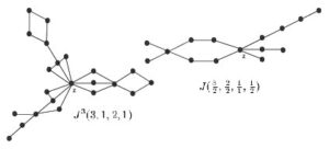
For illustration, we present the above matrix for the family of graphs represented by \(J^3(3,1,2,1)\). We also provide vertex ordering \(x_0,x_1,\ldots,x_{n-1}\) and the optimal radio labeling, which are obtained from this matrix.

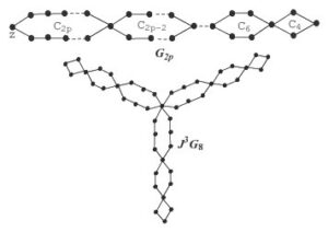
We end this section by computing the radio number of a cactus graph using Theorem 1. A cactus is a graph whose maximal connected subgraphs without a cut-vertex are cycles or complete graphs on two vertices. Let \(G_{2p}\) be the graph obtained by adjoining even cycles \(C_{2p},C_{2p-2},\ldots, C_4\) as shown in Figure 3. Let \(J^kG_{2p}\) be the wedge sum of \(k\geq2\) copies of \(G_{2p}\). The level tuple of \(G_{2p}\) is \((l_1,l_2,\ldots,l_r)\), where \(l_i=1\) for \(i\in\Big\{\frac{s(2p-s+1)}{2} \ : \ 1\leq s\leq p-1\Big\}\) and \(l_i=2\) otherwise. For instance, the level tuple of \(G_8\) is \((2,2,2,1,2,2,1,2,1)\). The level tuple of \(G_{2p}\) satisfies the condition of Theorem 1. For \(J^kG_{2p})\), we have \(d=(p-1)(p+2)\), \(n=k(p^2-1)+1\) and \(\sum_{s=1}^{r} sl_s=\frac{p(p^2-1)(3p+2)}{12}\). Thus, we have: \[rn(J^kG_{2p})=2+\frac{k(3p^2+4p-6)(p^2-1)}{6}.\]

3. Radio number of \(J\left(\frac{l_1}{l’_1},\frac{l_2}{l’_2},\ldots,\frac{l_r}{l’_r}\right)\)

Now we compute the radio number for some classes of \(J(\frac{l_1}{l’_1},\frac{l_2}{l’_2},\ldots,\frac{l_r}{l’_r})\). For this, we need some preliminaries.

Definition 6. Let \(G\) be any graph and let \(l\) be the level function defined on \(V(G)\) w.r.t. a vertex \(z\in G\). Then the sum \(w_z(G):=\sum_{v\in V(G)}l(v)\) is called the weight of the vertex \(z\).

Definition 7. The number \(w(G):=\min\{w_z(G) \ : z\in V(G) \}\) is called the weight of the graph \(G\). A vertex \(z\in V(G)\) is called a weight center of \(G\) if \(w_z(G)=w(G)\).

We use the following results which are proved in [10].

Proposition 1. For \(z,u\in V(G)\), we have \[w_z(G)-w_u(G)\leq(n-2n_u)d(z,u),\] where \(n_u=\big|\{v\in V(G) \ : \ d(u,v)=d(u,z)+d(z,v)\}\big|\) and \(n=|V(G)|\). In particular, \(z\) is a weight center if \(n_u\geq n/2\) for all \(u\in V(G)\).

Theorem 2. Let \(G\) be any graph on \(n\) vertices having diameter \(d\). Then \[rn(G)\geq 2 +(n-1)(d+1)-2w(G).\]

The similar lower bound is determined in [12] for trees. We first establish the lower bound for the radio number of \(J(\frac{l_1}{l’_1},\frac{l_2}{l’_2},\ldots,\frac{l_r}{l’_r})\) using the above theorem.

Proposition 2. Let \(G=J\left(\frac{l_1}{l’_1},\frac{l_2}{l’_2},\ldots,\frac{l_r}{l’_r}\right)\). Then \(w(G)=\sum_{s=1}^r s(l_s+l’_s)\) and consequently \[rn(G)\geq 2+(n-1)(d+1)-2\big[\sum_{s=1}^r s(l_s+l’_s)\big].\]

Proof. To prove our claim, it is sufficient to prove that the identified vertex \(z\) is a weight center of \(G\). For this, we use Proposition 1. Let \(u\in V(H)\). Then for any \(v\in V(H’)\), we have \(d(u,v)=d(u,z)+d(z,v)\). This means that \(n_u\geq |V(H’)|\) and consequently \(n_u\geq n/2\) for all \(u\in V(H)\). On the same lines, we have \(n_u\geq n/2\) for all \(u\in V(H’)\), showing that \(z\) is a weight center of \(G\). Hence the proof is complete.

Now we show that the above bound is optimal. For this, we use the following handy result.

Lemma 2. Let \(G=J\left(\frac{l_1}{l’_1},\frac{l_2}{l’_2},\ldots,\frac{l_r}{l’_r}\right)\) and let \(z=x_0\), \(x_1,\ldots,x_{n-1}\) be a labeling of \(V(G)\) such that for \(p>0\),

1. \(x_p\in H\) if \(p\) is odd, \(x_p\in H’\) otherwise, and
2. \(l(x_{p})+l(x_{p+1})\leq r+1\).

Then \[c(x_p)=1+p(d+1)+l(x_p)-2\sum_{s=1}^{p}l(x_s), \ 0\leq p\leq n-1\] is a radio labeling. Moreover, if \(l(x_{n-1})=1\) then \(c\) is optimal and \[rn(G)=c(x_{n-1})=2+(n-1)(d+1)-2\big[\sum_{s=1}^r s(l_s+l’_s)\big].\]

Proof. Let \(p>q\geq0\) have different parity. Then \(x_p\), \(x_q\) belongs to different graphs, \(H\) and \(H’\). In this situation, we have \(d(x_p,x_q)=l(x_p)+l(x_q)\). Therefore: \[c(x_p)-c(x_q)+d(x_p,x_q)=(p-q)(d+1)-2\big[\sum_{s=q+1}^{p-1}l(x_s)\big].\] Since \(l(x_s)\leq r\) and \(d=2r\), we obtain: \[c(x_p)-c(x_q)+d(x_p,x_q)\geq d+(p-q)\geq d+1.\] Now let \(p>q\geq0\) have same parity. Then either \(x_p,x_q\in H\) or \(x_p,x_q\in H’\). In both cases, we can write \[c(x_p)-c(x_q)=(p-q)(d+1)-\big[\sum_{s=q}^{p-1}l(x_s)+l(x_{s+1})\big].\] Using condition 2 and the fact that \(d=2r\), we get \(c(x_p)-c(x_q)\geq(p-q)r\). Since \(p,q\) have same parity, we have \(p-q\geq2\). Thus \(c(x_p)-c(x_q)\geq d\), showing that \(c\) is indeed a radio labeling. Moreover, \(c(x_p)>c(x_q)\) for \(p>q\) and \(l(x_{n-1})=1\). Thus, we have \[span(c)=c(x_{n-1})=2+(n-1)(d+1)-2\sum_{s=1}^{n-1}l(x_s).\] Since \(w(G)=\sum_{s=1}^{n-1}l(x_s)\), from Theorem 2 and Proposition 2, we obtain the desired result.

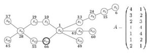
Similar to the case of \(J^k(l_1,l_2,\ldots,l_r)\), we provide an ordering of the vertices of \(J\left(\frac{l_1}{l’_1},\frac{l_2}{l’_2},\ldots,\frac{l_r}{l’_r}\right)\) represented by \(x_0,x_1,\ldots,x_{n-1}\), which satisfies the conditions of Lemma 2. In this case, we construct the following matrix: \[A=\left(\begin{array}{cc} l(x_1) \ \ & l(x_2) \\ l(x_3) \ \ & l(x_4)\\ \vdots & \vdots \\ l(x_{n-2}) \ \ & l(x_{n-1}) \end{array}\right),\] where columns consist of the following entries, respectively: \[\underbrace{r,r,\ldots,r}_{l_r-times}, \ \underbrace{r-1,r-1,\ldots,r-1}_{l_{r-1}-times}, \ \ldots, \ \underbrace{2,2,\ldots,2}_{l_2-times}, \ \underbrace{1,1,\ldots,1}_{l_1-times},\] \[\underbrace{r,r,\ldots,r}_{l’_r-times}, \ \underbrace{r-1,r-1,\ldots,r-1}_{l’_{r-1}-times}, \ \ldots, \ \underbrace{2,2,\ldots,2}_{l’_2-times}, \ \underbrace{1,1,\ldots,1}_{l’_1-times}\] such that \(l(x_i)+l(x_{i+1})\leq r+1\) and \(l(x_{n-1})=1\). We compute the radio number of \(J\left(\frac{l_1}{l’_1},\frac{l_2}{l’_2},\ldots,\frac{l_r}{l’_r}\right)\) when: Note that according to the definition of \(J\left(\frac{l_1}{l’_1},\frac{l_2}{l’_2},\ldots,\frac{l_r}{l’_r}\right)\), we also have the following implicit condition: \[\sum_{i=1}^r l_i=\sum_{i=1}^r l’_i.\] For even and odd values of \(r\), the above classes of \(J\left(\frac{l_1}{l’_1},\frac{l_2}{l’_2},\ldots,\frac{l_r}{l’_r}\right)\) can be represented as follows, respectively: \[J(\frac{a_1+\delta_1+1}{a’_1+\delta’_1+1},\frac{a_2+\delta_2}{a’_2+\delta’_2},\ldots,\frac{a_\theta+\delta_\theta}{a’_\theta+\delta’_\theta}, \frac{a’_\theta}{a_\theta},\frac{a’_{\theta-1}}{a_{\theta-1}},\ldots,\frac{a’_1}{a_1} ),\] \[J(\frac{a_1+\delta_1+1}{a’_1+\delta’_1+1},\frac{a_2+\delta_2}{a’_2+\delta’_2},\ldots,\frac{a_{\theta-1}+\delta_{\theta-1}}{a’_{\theta-1}+\delta’_{\theta-1}}, \frac{a}{a},\frac{a’_{\theta-1}}{a_{\theta-1}},\ldots,\frac{a’_1}{a_1} ),\] where \(a_i,a’_i,a>0\) and \(\delta_i,\delta’_i\geq0\) with \(\sum_i \delta_i=\sum_i\delta’_i\).

Theorem 3. Let \(G=J(\frac{l_1}{l’_1},\frac{l_2}{l’_2},\ldots,\frac{l_r}{l’_r})\) be as given in (6) and (7). Then \[rn(G)=2+(n-1)(d+1)-2\big[\sum_{s=1}^r s(l_s+l’_s)\big].\]

Proof. We only need to construct matrix \(A\) as mentioned above. The required matrix \(A=[C \ D]\), where: \[\begin{array}{rl} C=\left[\begin{array}{c} r\\r-1\\ \vdots \\ \theta+1 \\ \theta \\ \theta-1\\ \vdots \\ 1\\ 1 \\ 2 \\ \vdots \\ \theta-1 \\ \theta \end{array}\right] & \begin{array}{l} l_r\\l_{r-1}\\ \vdots \\ l_{\theta+1} \\ l’_{r+1-\theta} \\ l’_{r+2-\theta}\\ \vdots \\ l’_r\\ l_1-l’_r \\ l_2-l’_{r-1} \\ \vdots \\ l_{\theta-1}-l’_{r+2-\theta} \\ l_{\theta}-l’_{r+1-\theta} \end{array}\end{array} \mbox{ and } \begin{array}{rl} D=\left[\begin{array}{c} 1\\2\\ \vdots \\ r-\theta \\ r+1-\theta \\ r+2-\theta\\ \vdots \\ r\\ 2 \\ 3 \\ \vdots \\ \theta \\ 1 \end{array}\right] & \begin{array}{l} l_r\\l_{r-1}\\ \vdots \\ l_{\theta+1} \\ l’_{r+1-\theta} \\ l’_{r+2-\theta}\\ \vdots \\ l’_r\\ l’_2-l_{r-1} \\ l’_3-l_{r-2} \\ \vdots \\ l’_{\theta}-l_{r+1-\theta} \\ l’_1-l_{r} \end{array}\end{array}\] Evidently the above matrix satisfies the desired conditions. Hence the proof.

The above matrix, corresponding vertex ordering \(x_0,x_1\ldots,x_{n-1}\) and the optimal radio labeling for \(J(\frac{3}{2},\frac{2}{2},\frac{1}{1},\frac{1}{2})\), are shown in Figure 4.

We conclude by computing the radio number of a caterpillar using the above theorem. A caterpillar is a tree such that removing all its leaves, results in a path graph. Let \(CP(p_1,p_2,\ldots,p_s)\) be the caterpillar obtained from the path graph \(v_1v_2,v_2v_3,\ldots,v_{s-1}v_s\) by attaching \(p_i\geq0\) new terminal vertices to the vertex \(v_i\). For \(p_1,p_r>0\), the caterpillar \[G=CP(p_1,p_2,\ldots,p_{r-1},p_r+p_1,p_2,p_3,\ldots,p_r)\] is an example of \(J\left(\frac{1+p_1}{1+p_r},\frac{1+p_2}{1+p_{r-1}},\ldots,\frac{1+p_{r-1}}{1+p_2},\frac{p_r}{p_1}\right)\). For the caterpillar \(G\), we have \(n=2(r+p)-1\), \(d=2r\), \(w(G)=r^2+(p-1)r+p\) and \[rn(G)=2r(r+p), \] where \(p=p_1+p_2+\cdots+p_r\).

Acknowledgments : The second author was supported by the Higher Education Commission (Islamabad) through the National Research Program for Universities, Grant No. 7359/Punjab/NRPU/R\&D/HEC/2017.

Conflicts of Interest:

The authors declare no conflict of interests.

References:

1. Hale, W.K., 1980. Frequency assignment: Theory and applications. Proceedings of the IEEE, 68(12), pp.1497-1514. [Google Scholor]
2. Chartrand, G., Erwin, D., Harary, F. and Zhang, P., 2001. Radio labelings of graphs. Bulletin of the Institute of Combinatorics and its Applications, 33, pp.77-85.[Google Scholor]
3. Ahmad, A. and Marinescu-Ghemeci, R., 2017. Radio labeling of some ladder related graphs. Mathematical Reports (Bucuresti), 19(69), pp.107-119. [Google Scholor]
4. Bantva, D., 2017. Further results on the radio number of trees. Electronic Notes in Discrete Mathematics, 63, pp.85-91. [Google Scholor]
5. Bantva, D., 2017. Radio number for middle graph of paths. Electronic Notes in Discrete Mathematics, 63, pp.93-100. [Google Scholor]
6. Bantva, D., Vaidya, S. and Zhou, S., 2015. Radio number of trees. Electronic Notes in Discrete Mathematics, 48, pp.135-141. [Google Scholor]
7. Kang, S.M., Nazeer, S., Nazeer, W. and Lee, B.Y., 2015. Radio number of caterpillar graphs. Wulfenia, 22(5), pp.48-58. [Google Scholor]
8. Lo, M.L. and Alegria, L.V., 2016. Radio number for fourth power paths. Involve, a Journal of Mathematics, 9(2), pp.317-332. [Google Scholor]
9. Naseem, A. and Shabbir, K., 2020. The radio number for wedge sum of graphs. Ars Combinatoria, 151, pp.109-122. [Google Scholor]
10. Naseem, A., Shabbir, K. and Shaker, H., 2018. The radio number of edge-joint graphs. Ars Combinatoria, 139, pp.337-351.[Google Scholor]
11. Gallian, J.A., 2018. A dynamic survey of graph labeling. Electronic Journal of Combinatorics, 1(Dynamic Surveys), p.DS6. [Google Scholor]
12. Liu, D.D.F., 2008. Radio number for trees. Discrete Mathematics, 308(7), pp.1153-1164. [Google Scholor]