
The chromatic number of a graph is the minimum number of colors one needs to color the vertices of the graph such that no two adjacent vertices receive the same color. This can be thought of as paying 1 unit per color, but getting unlimited usage of each color. We consider here the scenario where the amount one pays for using a color is a function of how many times the color is used. This models for example scheduling problems where the cost of a resource depends on its usage; see for example [2, 3].
For \(m>0\) we let \(f(m)\) denote the cost of using any particular color \(m\) times. We call the \(f\) the cost-function. For example, for ordinary coloring \(f(m)=1\) for all \(m\). Given a proper \(k\)-coloring of the graph with the \(j\)th color used \(m_j\) times, the cost of the coloring is \(\sum\limits_j^k f(m_j)\). For a fixed cost-function \(f\), we define the \(f\)-chromatic number of \(G\), denoted \(\chi_f(G)\), as the minimum cost of a (proper) coloring of graph \(G\). We call a coloring achieving the minimum an \(f\)-optimal (or just optimal) coloring.
We require that a cost-function be non-decreasing. Further, for a given cost-function, the marginal costs are defined by \(c_i = f(i) – f(i-1)\) for \(i\ge 1\) (where we define \(f(0)=0\)). That is, \(c_i\) is the cost of the \(i\)th usage of a color. Thus \(f(m) = \sum\limits_{i=1}^m c_i\). We focus on the case that we call marginal-cost-decreasing (MCD), though to be more accurate it should be called marginal-cost-not-increasing. That is, \[c_i \ge c_j \quad\mbox{for all $i< j$.}\]
Since the cost-function is non-decreasing, all marginal costs are non-negative. Note that ordinary coloring has a cost-function that is MCD, since \(c_1=1\) and \(c_i=0\) for all \(i>1\).
In particular, being MCD implies that the cost-function \(f\) is sub-additive (meaning \(f(n+m) \le f(m)+f(n)\)). More generally, there are convexity conditions such as \[f( \ell + 1 ) + f( m – 1) \le f( \ell ) + f ( m ) \quad\mbox{for all $\ell \ge m$.} \label{eq:convex} \tag{1}\]
This follows since, if one has already \(\ell\) vertices with the first color and \(m-1\) with the second color, then giving the next vertex the first color costs \(c_{\ell+1}\), but giving it the second color costs \(c_m\), and we are assuming that \(c_{\ell+1} \le c_m\).
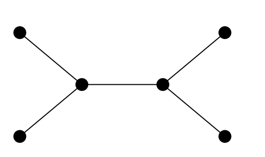
For a simple example, consider the tree \(D_6\) of order \(6\) with two vertices of degree \(3\) (See Figure 1). The natural bipartite coloring of \(D_6\) costs \(2f(3)\). But there is also a coloring where all four end-vertices receive the same color. This coloring has cost \(f(4)+2f(1)\). The latter coloring is cheaper if, for example, \(c_1=c_2=c_3=1\) and \(c_4=0\). In general, the usage is a partition of \(n\), the order, and we will sometimes write it as a vector \((a,b,c.\ldots)\) in non-increasing order. So, for example, the optimal coloring for the tree \(D_6\) is the cheaper of \((3,3)\) and \((4,1,1)\).
There has been work on the topic of what we here call cost-functions, though the research has largely focussed on the associated complexity questions. A general setting is a cost-function of the form \(2^V \to \mathbb{R}\); that is, a function that assigns a cost to each potential independent set. This setting was investigated for example by Sen et al. [8], Fukunaga et al. [2, 3], and in the equivalent clique-partitioning formulation, by Correa and Megow [1]. Our situation is what Fukunaga et al. call “monotone concave” (and it coincides with what Gijswijt et al. [4] call “value-polymatroidal” for the restricted situation that we are looking at). Other examples of cost-functions include the bounded vertex colorings of Hansen et al. [5] (but that version is not MCD) and also situations where different colors have different costs, most notably chromatic sum (see for example [6]).
We focus on bounds for general graphs and for specific classes of graphs. We also consider the number of colors that one actually uses in an optimal coloring (which is called the strength in the chromatic sum problem and the cost-chromatic number in [7]). In Section 2 we provide some elementary bounds and calculations for specific graphs. In Section 3 we focus on trees, and in Section 4 we consider the effect of several graph operations. In Section 5 we consider a specific example cost-function as a case study, and in Section 6 we briefly consider cost-functions more general than MCD along with possible future work.
For the complete graph \(K_n\) on \(n\) vertices, it holds that \(\chi_f(K_n) = nf(1)\) since there is only one coloring. Since an optimal coloring of \(G\) remains a proper coloring when restricted to any subgraph, it follows that:
Lemma 2.1. Given a cost-function \(f\), if \(H\) is a subgraph of graph \(G\), then \(\chi_f( H ) \leq \chi_f( G )\).
We observe next that one can assume that one has a “Grundy” coloring: that is, if one numbers the colors in non-increasing order of usage, then every vertex has a neighbor with each lower-numbered color.
Lemma 2.2. Given an MCD cost-function \(f\), for every graph \(G\) there is an optimal coloring of \(G\) that is a Grundy coloring.
Proof. Number the colors in non-increasing usage \((m_i)\). If a vertex \(v\) with color number \(j\) has no neighbor with color number \(k\) for some \(k<j\), then recoloring \(v\) with color \(k\) cannot increase the total cost, by Inequality (1). ◻
As a consequence it follows:
Lemma 2.3. Given an MCD cost-function \(f\), for every graph \(G\), there is an optimal coloring of \(G\) that uses at most \(\Delta+1\) colors, where \(\Delta\) is the maximum degree of \(G\).
Proof. A Grundy coloring uses at most \(\Delta+1\) colors. ◻
We continue with some elementary calculations.
Lemma 2.4. Given an MCD cost-function \(f\), for the complete bipartite graph \(K_{\ell,m}\), it holds that \(\chi_f(K_{\ell,m}) = f(\ell) + f(m)\).
Proof. Suppose two different colors are used in the same partite set. Then we noted in the introduction that sub-additivity implies that is not more expensive to merge the colors (that is, use the same color on their union). So one may assume that every pair of vertices in the same partite set have the same color. In other words, the natural bipartite coloring is optimal. It incurs a cost of \(f(\ell) + f(m)\). ◻
For example, for a star \(S_n\) with \(n-1\) leaves, it holds that \(\chi_f(S_n) = f(n-1) + f(1)\).
Lemma 2.5. Given an MCD cost-function \(f\):
(a) For the path \(P_n\) on \(n\) vertices it holds that \(\chi_f(P_n) = 2 f( n/ 2 )\) if \(n\) is even, and \(\chi_f(P_n) = f ((n+1)/2) + f( (n-1)/2 )\) if \(n\) is odd.
(b) For the cycle \(C_n\) on \(n\) vertices it holds that \(\chi_f( C_n) = 2 f( n/2 )\) if \(n\) is even, and \(\chi_f( C_n) = 2 f( (n-1)/2 ) + f(1)\) if \(n\) is odd.
Proof. (a) The natural bipartite coloring has the stated cost. Consider any coloring with usage vector \((m_i)\); its cost is \(\sum\limits_{i} f( m_i )\). We claim that this sum is at least the stated cost. Note that the path has independence number \(\lceil n/2 \rceil\); thus \(m_1 \le \lceil n/2 \rceil\). If \(m_1<\lceil n/2 \rceil\), then by Inequality (1), increasing \(m_1\) and decreasing \(m_2\) does not increase the overall sum. So one may assume that \(m_1 = \lceil n/2 \rceil\). By a similar argument, one may assume \(m_2 = n – m_1\). The claim follows.
(b) The natural coloring that uses the first two colors as much as possible has the stated cost. Again it holds that the total cost is at most the sum \(\sum\limits_{i} f( m_i )\). Here \(m_i \le \lfloor n/2 \rfloor\). And so on, as before. ◻
The lower bound argument in the calculation of the path and cycle in Lemma 2.5 can be re-used to show:
Lemma 3.1. Given an MCD cost-function \(f\), if \(G\) is a graph with order \(n\) and independence number \(\alpha\), it holds that \(\chi_f(G) \ge s f( \alpha) + f( n – s \alpha)\) where \(s = \lfloor n/\alpha \rfloor\).
Proof. As before, the coloring with usage vector \((m_i)\) has cost \(\sum\limits_{i} f( m_i )\). Each of the \(m_i\) is at most \(\alpha\). And again in providing a lower bound for the sum, one may assume \(m_1\) is as large as possible, and subject to this \(m_2\) is as large as possible, and so on. ◻
It follows that:
Lemma 3.2. Given an MCD cost-function \(f\), in the family of trees (and indeed connected bipartite graphs) of order \(n\), the star has minimum \(f\)-chromatic number and the path has maximum \(f\)-chromatic number.
Proof. For the upper bound, note that the natural bipartite coloring has cost \(f(m)+f(n-m)\) for some \(m\). By Inequality (1) this is at most the value for the path.
For the lower bound, we noted that \(f(\alpha) + f( n-\alpha)\) is a lower bound. By Inequality (1) this is at least \(f(n-1)+f(1)\), the value for the star. ◻
Indeed, the star has the least \(f\)-chromatic number among all connected graphs of that order.
We show next that the reason for the phenomenon exhibited by the tree \(D_6\) is that its maximum independent set is not one of the partite sets:
Theorem 3.3. Let \(T\) be a tree with order \(n\) and independence number \(\alpha\).
(a) If \(\alpha\) equals the size of the larger partite set, then for every MCD cost-function \(f\) the bipartite coloring of \(T\) is optimal.
(b) If \(\alpha\) is larger than the size of both partite sets, then there exists an MCD cost-function \(f\) such that every optimal \(f\)-coloring of \(T\) uses at least three colors.
Proof. (a) It follows from Lemma 3.1 that the \(f\)-chromatic number is at least \(f(\alpha) + f( n-\alpha)\); thus the bipartite coloring is optimal since it achieves that cost.
(b) Consider the cost-function \(f\) that has \(c_1=c_2= \ldots c_{\alpha-1} = 1\) and \(c_\alpha=0\). Then the bipartite coloring costs \(n\). But any coloring that gives all vertices in some maximum independent set the first color costs \(n-1\). And since the maximum independent set is not a vertex cover, one needs at least two more colors. ◻
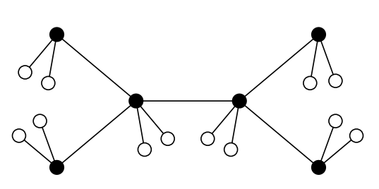
The above lemma shows that there are many trees where three colors are sometimes needed for an optimal coloring. In fact, one can go further. For a graph \(G\), we define a multi-corona of \(G\) as the graph obtained from \(G\) by adding at least two end-vertices adjacent to each vertex of \(G\). For example, Figure 2 shows one possible multi-corona of \(D_6\).
We will need the following simple observation:
Lemma 3.4. If \(f\) is an MCD cost-function with marginal costs \(c_i\), then for any positive constants \(a\) and \(b\), the cost-function \(f'\) with marginal costs \(ac_i+b\) is also MCD. Further, a coloring is \(f\)-optimal if and only it is \(f'\)-optimal.
This enables us to construct a cost-function where all end-vertices of a multi-corona receive the same color:
Lemma 3.5. Assume one has an MCD cost-function \(f\), a graph \(G\) of order \(n\), and a multi-corona \(G'\) of \(G\) of order \(N\). If cost-function \(f'\) is defined by marginal costs \(c'_i = 1 + c_i/(2c_1 N)\) if \(i\le n\) and \(c'_i=0\) if \(i>n\), then the optimal \(f'\)-coloring for \(G'\) is to give all end-vertices the same color and to use an optimal \(f\)-coloring of \(G\) on the subset \(V(G)\).
Proof. Consider a coloring of \(G'\) and let \(x\) be the number of vertices of \(G'\) that incur a marginal cost that is not zero. Then since each \(c_i < 1 + 1/N\), the total cost of the coloring is at least \(x\) but less than \(x+1\). Hence the optimal coloring of \(G'\) must minimize \(x\). That is, it must maximize the number of vertices with marginal cost zero. Since \(G'\) has a unique maximum independent set, this is uniquely attained by giving all end-vertices the same color. By the above lemma, what remains must be an optimal \(f\)-coloring of \(V(G)\). ◻
For example, for the multi-corona of \(D_6\) (shown in Figure 2), four colors are needed for the optimal coloring when the cost-function has marginal costs \(c_1=c_2=c_3=7/6\), \(c_4=c_5=c_6\), and \(c_i=0\) for \(i\ge 7\).
Lemma 3.6. For all positive integers \(k\) there is a tree \(T_k\) and an MCD cost-function \(f_k\) such that the optimal coloring of \(T_k\) uses \(k\) colors.
Proof. Apply the multi-corona repeatedly. ◻
We note that this construction is similar to one given by Mitchem and Morriss [7]. Interestingly, they study the situation where the colors have different cost-functions, but each cost-function is linear. Though this is different to ours, several of their results also hold here and with essentially the same proof. For example, we next re-use the technique given in the proof of Theorem 15 of [7].
Theorem 3.7. Given an MCD cost-function \(f\), for a tree \(T\) of maximum degree \(\Delta\), there is an optimal coloring of \(T\) that uses at most \(\lceil \Delta/2\rceil+1\) colors.
Proof. Suppose every optimal coloring of \(T\) uses more than \(\lceil \Delta/2\rceil+1\) colors; say the fewest colors is \(m\). Number the colors \(1\) up to \(m\) in order of non-increasing usage. Out of all optimal colorings using \(m\) colors, choose one which uses the \(m\)th color the least.
Consider a vertex \(v_0\) with the \(m\)th color. If \(v_0\) is missing a color in its neighborhood, then one can recolor it with a smaller-number color, without the cost increasing, a contradiction either of the optimality of the coloring or of the choice of optimal coloring. So \(v_0\) has neighbors of all other colors. Since \(2(m-2) \ge \Delta\), there must be a vertex \(v_1\) that is the only neighbor of \(v_0\) of that color. Similarly, either \(v_1\) misses a color, or it has a neighbor \(v_2\) that is the only neighbor of that color, except possibly \(v_0\). We create a sequence/path \(v_0, v_1, \ldots\). When we consider \(v_i\), either it is missing a color other than the \(m\)th color, or it has a neighbor \(v_{i+1}\) whose color does not appear anywhere else in the neighborhood except possibly on \(v_{i-1}\). Since \(T\) is a finite tree, this process must terminate. Assume it terminates at vertex \(v_r\) that is missing some color other than the \(m\)th color; say the \(k\)th color.
Then recolor the tree \(T\) by assigning \(v_i\) the color of \(v_{i+1}\) for \(0 \le i < r-1\), and giving \(v_r\) its missing color \(k\). This remains a proper coloring. The net change in usage is increased usage of the \(k\)th color and reduced usage of the \(m\)th color. Again this contradicts either the optimality or the choice of optimal coloring. That is, our original supposition is false. ◻
Here we consider how some operations affect the \(f\)-chromatic number. Consider adding an edge to the graph. It is immediate that \(\chi_f(G + e) \ge \chi_f(G)\), since any coloring of \(G+e\) is also a coloring of \(G\) (as observed earlier). At the same time, one can recolor one of the ends of \(e\) with a new color. So \(\chi_f( G + e ) \le f(1) + \chi_f (G )\). This can be achieved, as it is for ordinary chromatic number.
In another direction, a formula for the join of two graphs is trivial. Since the colors used on the constituent graphs are disjoint, it holds that \(\chi_f( G \vee H) = \chi_f(G) + \chi_f(H)\).
For two disjoint copies of a graph, the ordinary chromatic number is just the same as the original. Here, there is an inequality \(\chi_f( 2G ) \le 2 \chi_f(G)\); simply replicate the coloring. This bound cannot be improved, as for example, if \(f(m)=m\) then \(\chi_f\) equals the number of vertices. But in fact, the replicate coloring is optimal:
Theorem 4.1. Given an MCD cost-function \(f\), for any graph \(G\) an optimal coloring of \(2G\) is obtained by using the optimal coloring of \(G\).
Proof. Consider a coloring that is not identical on the two copies \(G_1\) and \(G_2\). Say one has usage \((a_i)\) on \(G_1\) and \((b_i)\) on \(G_2\). Then we claim that for each \(i\) one has \(2f(a_i+b_i) \ge f(2a_i) + f(2b_i)\) by concavity. (Say \(a_i<b_i\). Then \(LHS = 2\sum\limits_{j=1}^{a_i+b_i} c_j\) while \(RHS = \sum\limits_{j=1}^{2a_i} c_j \,+\, \sum\limits_{j=1}^{2b_i} c_j\); thus \(RHS-LHS = \sum\limits_{j=a_i+b_i+1}^{2b_i} c_j \,-\, \sum\limits_{j=2a_i+1}^{a_i+b_i} c_j \le 0\).)
It follows that, either copying the coloring on \(G_1\) onto \(G_2\), or vice versa, is no worse than the current optimal coloring. ◻
The situation seems more complicated when one considers the disjoint union of two different graphs.
We observed that the multi-corona has interesting properties. Another version of the corona is also interesting. Given graph \(G\) and integer \(\ell \ge 2\), construct graph \(W_\ell(G)\) as follows: take \(G\), and for each vertex \(v\) of \(G\) introduce a clique of \(\ell-1\) vertices with \(v\) adjacent to all vertices of its clique.
Lemma 4.2. Let MCD cost-function \(f\) be given. If graph \(G\) has order \(n\) and integer \(\ell \ge 2\), then \(\chi_f ( W_\ell(G) ) \ge \ell f(n)\). Furthermore, there is equality in this bound if \(G\) is \(\ell\)-colorable; and if \(c_1 > c_n\) then this is the only case of equality.
Proof. The independence number of \(W_\ell(G)\) is \(n\). Thus, by Lemma 3.1, the total cost of the coloring is at least \(\ell f(n)\). If \(G\) has an \(\ell\)-coloring, then trivially this coloring can be extended to an \(\ell\)-coloring of \(W_\ell(G)\). Hence the cost of a optimal coloring of \(W_\ell(G)\) equals \(\ell f(n)\). If \(G\) does not have an \(\ell\)-coloring, then neither does \(W_\ell(G)\). Thus in any coloring thereof, the \(\ell\)th most used color is used less than \(n\) times. Since \(c_1 > c_{n}\), it follows that the optimum cost for \(W_\ell(G)\) in that case is more than \(\ell f(n)\). ◻
Turning to algorithmic questions, we note that the \(f\)-chromatic number problem is of course NP-complete, since it generalizes ordinary chromatic number. There are, however, degenerate \(f\) where the problem is trivial (such as all \(c_i=1\)). However, Fukunaga et al. (Theorem 4.5 of [3]) showed that this is the only such case. Their construction has similarities to the above construction.
Theorem 4.3. [3] Given an MCD function \(f\) such that the marginal costs are not constant, the \(\chi_f\)-coloring problem is NP-complete.
Fukunaga et al. [2, 3] also provided several approximation algorithms. For exact algorithms they showed that the greedy algorithm works on proper/unit interval graphs.
As an example parameter, we provide some results on the case that \(c_1=c_2=1\) and \(0=c_3=c_4 \ldots\). We define the twice-pay coloring number of a graph whereby one pays one unit for each of the first and second usages of a color and then usage is free there after. This is a special case of the “rent-or-buy” scenario investigated in [2].
Some bounds are immediate. For example, the parameter lies between \(\chi\) and \(2 \chi\). If a graph is connected with maximum degree \(\Delta\), then the parameter is at most \(2 \Delta +1\), with equality only for the odd cycles of length at least \(5\).
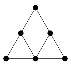
It is to be noted that the optimal twice-pay coloring might use more colors that the ordinary chromatic number. For a simple example, consider the \(3\)-sun formed by taking a \(6\)-cycle and adding edges to convert one of the maximum independent sets into a clique. Then there is a unique \(3\)-coloring, and it uses each color twice. But the twice-pay chromatic number is \(5\), attained by giving all three degree-\(2\) vertices the same color.
The maximum value of the parameter is \(n\), the order of the graph. The graphs with value \(n\) are exactly those with independence number at most \(2\). It is also easy to determine the connected graphs with small value. The parameter equals \(2\) if and only if the graph is \(K_2\), and equals \(3\) if and only the graph is a star. A connected graph has twice-pay coloring number \(4\) if and only if it is bipartite or has two adjacent vertices that form a vertex cover.
As with general MCD functions, the value for the join is the sum of the values of the originals. The value for the union is at most twice that of the original with equality only if the original graph is complete. In particular, the value for \(2G\) equals \(2\chi\). From this it follows that the decision problem for twice-pay chromatic number is NP-hard for values at least \(6\). The value for the cartesian product \(G \Box G\) at most twice the value for \(G\) (since the product has the same chromatic number), with equality only when \(G\) is complete.
One can provide bounds for some surfaces. For example, the value is at most \(8\) for planar graphs, by the 4-Color Theorem. Further, for toroidal graphs the value is at most \(11\), since Thomassen [9] showed that every toroidal graph with chromatic number at least \(6\) has a noncontractible triangle—and removing this triangle leaves a planar graph.
While our focus has been on MCD cost-functions, we noted before that other cost-functions have been proposed and studied. Some of these have a sub-additive cost-function, such as the rent-or-buy problem, investigated by Fukunaga et al. [2, 3]. There a typical cost-function is \(f(m)=m\) for \(m \le k\) and \(f(m)=k\) for \(m > k\) for some threshold \(k\). (The twice-pay number is where \(k=2\).) There are also situations that are not sub-additive, such as the bounded coloring of Hansen et al. [5]. With no constraint on the cost-function, other than being nondecreasing, even coloring the edgeless graph becomes an optimization problem, and there seems little to say about this in general.
Some of the results for MCD cost-functions generalize to sub-additive functions. But some only partially. For example, Lemma 2.5 gave the formula for paths and cycles, but the situation for sub-additive functions is a little more general:
Lemma 6.1. Given a sub-additive function \(f\), for the \(n\)-path and the \(n\)-cycle, there is an optimal coloring that uses at most three colors.
Proof. We provide the proof for the case of a path. The case of a cycle is similar.
We claim first that, for any non-increasing partition \((a_1,a_2,a_3)\) of \(n\) with biggest part \(a_1\le \lceil n/2\rceil\), there is a partition \((A_1,A_2,A_3)\) of the vertex set such such that each \(A_i\) is an independent set with \(|A_i| = a_i\). One recipe is to use induction to prove the claim with the added condition that the first vertex is in \(A_1\): if \(a_2>a_3\) then put the first vertex in \(A_1\) and the second in \(A_2\) and induct; else put the first three vertices in \(A_1\), \(A_2\), and \(A_3\) respectively and induct.
So to prove the lemma, if more than three colors are used, repeatedly combine the two smallest usages into one usage until one has only three usages. This combining cannot increase the cost, because of the sub-additive condition. And the resulting usage has a feasible coloring by the previous paragraph. ◻
For example, for the \(6\)-path or \(6\)-cycle the bipartite coloring is optimal for any MCD cost-function (though not necessarily unique). But for the sub-additive cost-function with \(f(1)=f(2)=1\) and \(f(3)=4/3\), using three colors is uniquely optimal.
We conclude with some possible future directions.
(a) What is the smallest order of a tree \(T\) such that there exists an MCD cost-function \(f\) where the optimal coloring of \(T\) needs four colors?
(b) Is there a subcubic graph where \(4\) colors are needed for some cost-function?
(c) For fixed cost-function \(f\), is there always a linear-time algorithm for trees?
(d) For a fixed graph, one can consider all possible MCD cost-functions \(f\) and the optimal colorings for each \(f\) and thence make a list of all coloring partitions that ever arise. This is a bit silly, since if \(c_i=1\) for all \(i\), then every proper coloring is optimal. So maybe one restricts to those cost-functions \(f\) where the optimal coloring partition is unique. How does this set grow? Behave? Consider it as a polytope?