
The foremost requirement before conducting an experiment is to choose the best suited combinatorial design, keeping in view the available resources and constraints. Due to the immense efforts of researchers, a large variety of experimental designs are available today, among which a best fit design can be chosen to conduct any experiment. There are complete block designs, incomplete block designs, row-column designs, factorial experiments, supersaturated designs, etc.
Partially Balanced Incomplete Block (PBIB) designs are an important type of incomplete block design. Initially proposed for agricultural experimentation, these designs have now a wide area of their applications. These designs have proven applications in agricultural experimentation, group testing, complete diallel crosses, sample surveys, key-predistribution, etc.
PBIB designs were first introduced by [1]. These designs are always based on some association scheme. Their first classification based on the type of association scheme was performed by [2]. Later, different types of association schemes were proposed and corresponding PBIB designs were constructed by different researchers. Notable among these researchers are [4, 6, 7, 9, 11], etc. In [5], basic magic squares were studied and some PBIB designs were constructed.
The present paper is written with an objective to explore the usefulness of magic squares and their properties in the construction of PBIB designs. In this direction, we have first proposed a new method for the construction of magic squares and discussed their properties. These properties have been later used in Section 4 to propose some new types of association schemes. We have also discussed the closeness of some existing association schemes with some other properties of magic squares. These properties are then used to construct four series of PBIB designs based on the newly proposed association schemes. At the end of the paper, we have prepared a table which enlists some of the PBIB designs constructed in this paper.
A magic square is an n\(\times\)n square matrix such that each of its cells contains an integer and the sum of the integers in its each row, column and diagonal is equal to some constant value. This constant is called the magic constant of the magic square. For a detailed study about different types of magic squares and the techniques used for their construction, we can refer to [3].
An n\(\times\)n Latin square can be defined as an n\(\times\)n square matrix comprising of integers 1, 2, …, n such that each of its rows and columns contains all the n integers exactly once.
The concept of association scheme was introduced by [2]. An m-associate class association scheme can be defined as below:
Given v symbols (treatments) 1, 2, …, v, a relation satisfying the following conditions is called an m-class association scheme (m \(\ge\) 2):
i. Any two symbols are either 1st, 2nd, … or m\(^{th}\) associates, the relation of association being symmetric, i.e., if the symbol \(\alpha\) is the i\(^{th}\) associate of \(\beta\), then \(\beta\) is the i\(^{th}\) associate of \(\alpha\).
ii. Each symbol \(\alpha\) has n\(_i\) i\(^{th}\) associates, the number n\(_i\) being independent of \(\alpha\).
iii. If any two symbols \(\alpha\) and \(\beta\) are i\(^{th}\) associates, then the number of symbols that are j\(^{th}\) asociates of \(\alpha\) and k\(^{th}\) associate of \(\beta\) are \(p^i_{jk}\) and are independent of the pair of i\(^{th}\) associates i.e., \(\alpha\) and \(\beta\).
The integers v, \(n_i\) and \(p^i_{jk}\) (i, j, k = 1, 2, …, m) are the parameters of the association scheme. The elements \(p^i_{jk}\) are represented by an m \(\times\) m matrix as follows: \[P_i =\begin{bmatrix} p^i_{11}& p^i_{12}& p^i_{13}&\ldots& p^i_{1m}\\ p^i_{21}& p^i_{22}& p^i_{23}&\ldots& p^i_{2m}\\ \vdots&\vdots&\vdots&\vdots&\vdots\\ p^i_{m1}& p^i_{m2}& p^i_{m3}&\ldots& p^i_{mm} \end{bmatrix},\] where, i = 1, 2, …, m.
These P\(_i\)’s (i = 1, 2, …, m) are called P-matrices of the association scheme.
The parameters of the association scheme are not all independent and are connected by the following relations: \[\begin{aligned} \sum_{i=1}^m n_i=&v-1;\\ \sum_{k=1}^m p^i_{jk}=&n_j-\delta_{ij}, \end{aligned}\] where \(\delta_{ij}\) is Kronecker’s delta and is defined as \(\delta_{ij}\) = 1 if \(i = j\) and \(\delta_{ij}\) = 0 if i \(\ne\) j.
\[n_i p^i_{jk} = n_j p^j_{ik},\qquad i, j, k = 1, 2, \ldots.., m.\]
If every symbol is taken as its \(0^{th}\) associate and of no other symbol, then
\[\begin{aligned}
n_0 =& 1;\\
p^0_{ij} =& n_i \delta_{ij};\\
p^i_{0k} =& \delta_{ik},
\end{aligned}\] where \(\delta_{ij}\) is Kronecker’s delta as
defined above. Then, the above parametric relations of the association
scheme can be revised as:
\[\begin{aligned}
\sum_{i=0}^m n_i =& v;\\
\sum_{i=0}^m p^i_{jk} =& n_j;\\
n_i p^i_{jk} =& n_j p^j_{ik},
\end{aligned}\] where i, j, k = 0, 1, 2, …, m.
Given an association scheme A with m-associate classes (m \(\ge\) 2) and v treatments, we have a PBIB design with b blocks, r replications and block size k based on A if it is possible to arrange the v treatments in b blocks such that
(a) each block contains k (k \(<\) v) distinct treatments;
(b) each treatment occurs in r blocks;
(c) if the treatments \(\alpha\) and \(\beta\) are mutually i\(^{th}\) associates in the association scheme, then \(\alpha\) and \(\beta\) occur together in \(\lambda_i\) blocks, where the integer \(\lambda_i\) does not depend on the pair \((\alpha, \beta)\) so long as they are mutually i\(^{th}\) associates, i = 1, 2, …, m. Further, not all \(\lambda_i\) ’s are equal.
The integers v, b, r, k, \(\lambda_i\) ( i = 1, 2, …, m) are the parameters of the PBIB design.
The following relations between the parameters of the association scheme and those of the PBIB designs are well known:
\[\begin{aligned} vr=&bk\\ \sum_{i=0}^m n_i\lambda_i=&rk, \end{aligned}\] where \(\lambda_0 = r.\)
It is clear from the above that the definition of a PBIB design is clearly based on the existence of an m-associate class association scheme which means that if for some values of v, m, n\(_i\) and \(p^i_{jk}\), there exists no m-associate class association scheme then there is no m-associate class PBIB design based on it.
For further details about association schemes and the PBIB designs, one can refer to [8].
In this section, we have proposed a new method in the form of Algorithm 3.1 which constructs n\(\times\)n magic squares using n\(\times\)n Latin squares. The method for the construction of required latin squares is also given in the form of Algorithm 3.2. The specialty of the proposed method for the construction of the magic squares is that the properties of magic squares can be fixed in advance through the Latin square being used. For example, to construct an n\(\times\)n magic square with each row, column, and forward and backward diagonal sum equal to its magic constant, we will use an n\(\times\)n Latin square such that each of its rows, columns and diagonals contains all the n integers (1, 2, …, n) exactly once.
A magic square can be constructed as follows:
Step 1. First of all, construct an n\(\times\)n Latin square keeping in view the desired properties of magic square to be constructed. For example, consider the following 4\(\times\)4 Latin square A. \[A=\begin{matrix} 1&2&3&4\\ 3&4&1&2\\ 4&3&2&1\\ 2&1&4&3 \end{matrix}\]
The above Latin square contains all the integers, i.e., 1, 2, 3, 4 in each of its rows, columns, and forward and backward diagonals. Moreover, its corner elements, and the corner 2\(\times\)2 square matrices contain all four of the integers. The central square matrix of order 2\(\times\)2 also contains all four of the integers.
Step 2. Now, take the transpose of Latin square A, change the notations of its entries and denote it by B. \[B = \begin{matrix} 1'&3'&4'&2'\\ 2'&4'&3'&1'\\ 3'&1'&2'&4'\\ 4'&2'&1'&3' \end{matrix}\]
The properties of Latin square B will be same as those of Latin square A.
Step 3. Now assign any integral values to the notations of entries (i.e., 1, 2, 3, 4 and \(1', 2', 3', 4'\)) used in Latin squares A and B.
Step 4. Now add matrix A to the matrix B. The resulting matrix will be a magic square with the properties fixed in step 1, i.e., the sum of each of its rows, columns, and the forward and backward diagonal will be equal to its magic constant. The sum of all the four corner entries and the sum of the elements in each of the four corner 2\(\times\)2 square matrices and central 2\(\times\)2 matrix will also be equal to its magic constant.
As an illustration, suppose \[A=\begin{matrix} 1&2&3&4\\ 3&4&1&2\\ 4&3&2&1\\ 2&1&4&3 \end{matrix}\] and \[B = \begin{matrix} 10&12&14&2\\ 2&14&12&10\\ 12&10&2&14\\ 14&2&10&12 \end{matrix}\]
Now following above algorithm, we obtain the following magic square, say, S \[S=A+B=\begin{matrix} 11&14&17&6\\ 5&18&13&12\\ 16&13&4&15\\ 16&3&14&15 \end{matrix}\]
Next, we will propose an algorithm to construct the type of Latin squares with properties similar to the Latin square A used in Step 1 of Algorithm 3.1.
This algorithm constructs a Latin square of order \(2^i\times2^i (i = 2, 3, \ldots)\). The steps involved uses a Latin square of order M\(\times\)M to construct a Latin square of order 2M\(\times\)2M.
Step 1. Use the Latin square of order M\(\times\)M to directly fill half of the cells of the first M rows of 2M\(\times\)2M Latin square such that the first M cells of the first row of the 2M\(\times\)2M Latin square are directly filled by the first row of M\(\times\)M Latin square in the same order. Now, the second row of the M\(\times\)M Latin square is used in the same order to fill the last M cells of the second row of the 2M\(\times\)2M Latin square. In the similar way, all the M rows of M\(\times\)M Latin square will fill the half of the cells in first M rows of the 2M\(\times\)2M Latin square such that odd numbered rows will be used to fill the first M cells of the corresponding odd number rows of the 2M\(\times\)2M Latin square and the even numbered rows will be used to fill last M cells of the corresponding even numbered rows of the 2M\(\times\)2M Latin square. For example, the Latin square A in step 1 of Algorithm 3.1 can be used to directly fill the half of the cells in first four rows of the \(8\times8\) Latin square as given below: \[\begin{matrix} 1&2&3&4&-&-&-&-\\ -&-&-&-&3&4&1&2\\ 4&3&2&1&-&-&-&-\\ -&-&-&-&2&1&4&3\\ -&-&-&-&-&-&-&-\\ -&-&-&-&-&-&-&-\\ -&-&-&-&-&-&-&-\\ -&-&-&-&-&-&-&- \end{matrix}\]
Step 2. Now, in each of the half filled rows, fill up the remaining half cells using the next M integral notations (i.e., M+1, M+2, …, 2M) in the same order as that of the order in which the previously half filled integers occur. For example, in the first row of the \(8\times8\) Latin square, the first four elements are integers 1 to 4 in the increasing order of their magnitudes. Therefore, next four elements will be the integers 5 to 8 in the same order, i.e., in the increasing order of their magnitudes. Similarly, we will fill all the remaining half filled (M – 1) rows and we will have: \[\begin{matrix} 1&2&3&4&5&6&7&8\\ 7&8&5&6&3&4&1&2\\ 4&3&2&1&8&7&6&5\\ 6&5&8&7&2&1&4&3\\ -&-&-&-&-&-&-&-\\ -&-&-&-&-&-&-&-\\ -&-&-&-&-&-&-&-\\ -&-&-&-&-&-&-&- \end{matrix}\]
Step 3. Now, once we have obtained the first M rows of the 2M\(\times\)2M Latin square, the last M rows can be obtained using the first M rows such that the (M+i)\(^{th}\) row is obtained from the i\(^{th}\) row (i = 1, 2, …, M) such that the (M+i)\(^{th}\) row contains the elements in the reverse order as that of the i\(^{th}\) row. For example, the \(5^{th}\) row of the above \(8\times8\) Latin square can be obtained from the \(1^{st}\) row by filling its cells in the reverse order as that of the \(1^{st}\) row. Therefore, the \(5^{th}\) row is: \[\begin{matrix} 8&7&6&5&4&3&2&1 \end{matrix}.\]
Now, repeat the same procedure to obtain all the remaining rows of the required \(8\times8\) Latin square. Now we have the following complete \(8\times8\) Latin square. \[\begin{matrix} 1&2&3&4&5&6&7&8\\ 7&8&5&6&3&4&1&2\\ 4&3&2&1&8&7&6&5\\ 6&5&8&7&2&1&4&3\\ 8&7&6&5&4&3&2&1\\ 2&1&4&3&6&5&8&7\\ 5&6&7&8&1&2&3&4\\ 3&4&1&2&7&8&5&6 \end{matrix}\]
The rows, columns, and the forward and backward diagonals of the above Latin square each contains all eight of the integers (i.e., 1, 2, …, 8) exactly once. All the four corner matrices of order \(4\times4\) contain all the eight integers exactly twice (because its order is \(2.4\times2.4\)). From each corner of the above \(2.4\times2.4\) magic square, if we take two elements, either row-wise or column-wise, then this set also contains all eight of the integers. The central \(4\times4\) square also contains all the eight integers twice.
Suppose now that we have a M\(\times\)M magic square constructed using above Algorithms 3.1 and 3.2. The structure of this magic square can be divided into four n\(\times\)n sub-squares and each n\(\times\)n sub-square can further be divided in four m\(\times\)m sub-squares as shown in Figure 1 below.

The magic squares constructed using Algorithm 3.1 and Algorithm 3.2 will have the following properties:
i. The sum of each row, each column and both diagonals will be equal which will be its magic constant.
ii. The magic square of order M\(\times\)M; where M = \(2^i\) and i = 2, 3, …; can be divided into four sub-squares of order n\(\times\)n ; where \(n = 2^i – 1\) such that sum of integers in each of these sub squares is equal to \(2^i -2\) times the magic constant.
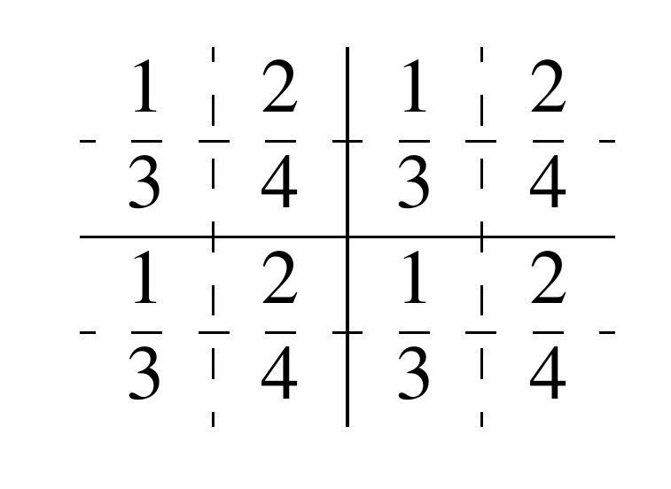
iii. Each of the n\(\times\)n sub squares can further be divided into four sub-squares of order m\(\times\)m; where \(m = 2^{i -2}\). Let us number them from 1 to 4 such that same positioned sub-matrices are assigned the same number.
The sum of all the integers in the same numbered the m\(\times\)m sub squares will be equal to \(2^{i – 2}\) times the magic constant. iv. The sum of central sub-square of order n\(\times\)n will also be equal to \(2^{i – 2}\) times the magic constant.
v. The corner \(2^{i – 2}\) integers in either order also add up to give the magic constant.
In this section, we have proposed some new association schemes using the properties of magic squares discussed in above section. These association schemes will later be used in Section 5 to construct some series of PBIB designs.
Before defining our association schemes, we assume that each distinct cell of M\(\times\)M magic square contains a distinct treatment and we assign each of these cells and thus treatments a distinct integral value in the increasing order of magnitude. For example, for a 4\(\times\)4 magic square, we have the following arrangement of 16 treatments: \[\begin{matrix} 1&2&3&4\\ 5&6&7&8\\ 9&10&11&12\\ 13&14&15&16 \end{matrix}\]
Using the property (ii) of magic squares as discussed in Subsection 3.3, we can define a new four-associate class association scheme as below:
i. Two treatments are mutually first associates if they belong to the same n\(\times\)n sub-square. For example, treatments in A\('\) are mutually first associates. See Figure 2.
ii. Two treatments are mutually second associates if they belong to two different horizontally positioned adjacent n\(\times\)n sub-squares. For example, in Figure 2, all the treatments in A\('\) are second associates of all the treatments in B\('\), and vice-versa.
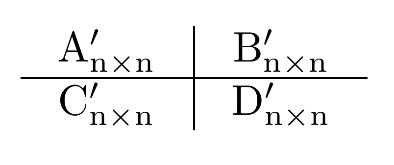
iii. Two treatments are mutually third associates if they belong to two different vertically positioned adjacent n\(\times\)n sub-squares. For example, all the treatments in A\('\) are third associates of all the treatments in C\('\), and vice-versa.
iv. Treatments which belong to two different diagonally positioned n\(\times\)n sub-squares are mutually fourth associates. For example, all the treatments in A\('\) are fourth associates of all the treatments in D\('\), and vice-versa.
Following are the generalized parameters of the above defined Association scheme 4.1.
\[\begin{aligned} v=&M^2,\\ n_1=&n^2-1,\\ n_2=&n_3=n_4=n^2, \end{aligned}\]
\[\begin{aligned} P_1&=\begin{bmatrix} n^2-2&0&0&0\\ 0& n^2&0&0\\ 0&0& n^2&0\\ 0&0&0& n^2 \end{bmatrix},\\ P_2&=\begin{bmatrix} 0& n^2-1&0&0\\ n^2-1&0&0&0\\ 0&0&0& n^2\\ 0&0& n^2&0 \end{bmatrix},\\ P_3&=\begin{bmatrix} 0&0& n^2-1&0\\ 0&0&0& n^2\\ n^2-1&0&0&0\\ 0& n^2&0&0 \end{bmatrix},\\ P_4&=\begin{bmatrix} 0&0&0& n^2-1\\ 0&0& n^2&0\\ 0& n^2&0&0\\ n^2-1&0&0&0 \end{bmatrix}. \end{aligned}\]
Now, using the property (iii) of magic squares, we can define a new two-associate class association scheme as given below:
i. For a given treatment \(\alpha\), those treatments are its first associates which belong to the same numbered m\(\times\)m sub-squares (refer to Figure 3). For example, if treatment \(\alpha\) belongs to an m\(\times\)m sub-square which has been assigned integral value 1, then all the other treatments which also belong to sub squares denoted by 1 are its first associates.
ii. All the remaining treatments are the second associates of treatment \(\alpha\).
The generalized parameters of the above defined two-associate class association scheme are given below \[\begin{aligned} v&= M^2 & n_1&= 4m^2-1& n_2&=12m^2\\ P_1&=\begin{bmatrix} 4m^2-2&0\\ 0&12m^2 \end{bmatrix} & P_2&=\begin{bmatrix} 0& 4m^2-1\\ 12m^2-1&0 \end{bmatrix} \end{aligned}\]
The above defined association scheme is also Pseudo Group Divisible association scheme with \(m=4\) and \(n=4m^2\).
The associate classes in above defined Association scheme 4.2 can be further partitioned to define a new four-associate class association scheme as given below:
i. Two treatments \(\alpha\) and \(\beta\) are mutually first associates if they belong to the same numbered m\(\times\)m sub-squares. For example, all the treatments in sub squares denoted by 1 are mutually first associates. See Figure 3.
ii. Second associates of a treatment \(\alpha\) are those treatments which belong to the m\(\times\)m sub-squares which are denoted by integral value as that of the m\(\times\)m sub-square which is positioned horizontally with respect to the m\(\times\)m sub-square to which treatment \(\alpha\) belongs, inside the same n\(\times\)n sub-square. For example, in Figure 3, for any treatment \(\alpha\) belonging to sub-square denoted by integral value 1, all those treatments in all the four sub-matrices denoted by integral value 2 are its second associates.
iii. Third associates of a treatment \(\alpha\) are those treatments which belong to m\(\times\)m sub-squares which are denoted by integral value as that of the m\(\times\)m sub-square which is positioned vertically with respect to the m\(\times\)m sub-square to which treatment \(\alpha\) belongs, inside the same n\(\times\)n sub-square. For example, for any treatment \(\alpha\) belonging to sub-matrix denoted by integral value 1, all those treatments in all the four sub-matrices denoted by integral value 3 are its third associated.
iv. Fourth associates of a treatment \(\alpha\) are those treatments which belong to m\(\times\)m sub-squares which are denoted by integral value as that of the m\(\times\)m sub-square which is positioned diagonally with respect to the m\(\times\)m sub-square to which treatment \(\alpha\) belongs, inside the same n\(\times\)n sub-square. For example, for any treatment \(\alpha\) belonging to sub-square denoted by integral value 1, all those treatments in all the four sub-matrices denoted by integral value 4 are its fourth associated.
The generalized parameters of the above defined four-associate class association scheme are as given below:
\[\begin{aligned} v=& M^2,\\ n_1=&4m^2-1,\\ n_2=&n_3=n_4=4m^2, \end{aligned}\] \[\begin{aligned} P_1&=\begin{bmatrix} 4m^2-2&0&0&0\\ 0&4m^2&0&0\\ 0&0&4m^2&0\\ 0&0&0&4m^2 \end{bmatrix},\\ P_2&=\begin{bmatrix} 0&4m^2-1&0&0\\ 4m^2-1&0&0&0\\ 0&0&0&4m^2\\ 0&0&4m^2&0 \end{bmatrix},\\ P_3&=\begin{bmatrix} 0&0&4m^2-1&0\\ 0&0&0&4m^2\\ 4m^2-1&0&0&0\\ 0&4m^2&0&0 \end{bmatrix},\\ P_4&=\begin{bmatrix} 0&0&0&4m^2-1\\ 0&0&4m^2&0\\ 0&4m^2&0&0\\ 4m^2-1&0&0&0 \end{bmatrix}. \end{aligned}\]
For magic squares of order \(2^i\times2^i\) (i = 3, 4, …), the associate classes in Association scheme 4.1 can be further extended using the properties (ii) and (iii) of magic squares to define a new five-associate class association scheme as given below:
i. Two treatments which belong to the same m\(\times\)m sub-square in the same the same n\(\times\)n sub-square are mutually first-associates.
ii. Two treatments \(\alpha\) and \(\beta\) are mutually second associates if they belong to the differently numbered m\(\times\)m sub-squares in the same n\(\times\)n sub-square.
iii. Two treatments are mutually third associates if they belong to two different horizontally positioned n\(\times\)n sub-squares.
iv. Two treatments are mutually fourth associates if they belong to two different vertically positioned n\(\times\)n sub-squares.
v. Treatments which belong to two different n\(\times\)n sub-squares positioned diagonally are mutually fifth associates.
The generalized parameters of the above defined five-associate class association scheme are as given below:
\[\begin{aligned} v=&M^2,\\ n_1=&m^2-1,\\ n_2=&3m^2,\\ n_3=&n_4=n_5=4m^2, \end{aligned}\] \[\begin{aligned} P_1&=\begin{bmatrix} m^2-2&0&0&0&0\\ 0&3m^2&0&0&0\\ 0&0&4m^2&0&0\\ 0&0&0&4m^2&0\\ 0&0&0&0&4m^2 \end{bmatrix},\\ P_2&=\begin{bmatrix} 0& m^2-1&0&0&0\\ m^2-1&2m^2&0&0&0\\ 0&0&4m^2&0&0\\ 0&0&0&4m^2&0\\ 0&0&0&0&4m^2 \end{bmatrix},\\ P_3&=\begin{bmatrix} 0&0& m^2-1&0&0\\ 0&0&3m^2&0&0\\ m^2-1&3m^2&0&0&0\\ 0&0&0&0&4m^2\\ 0&0&0&4m^2&0 \end{bmatrix}\\ P_4&=\begin{bmatrix} 0&0&0& m^2-1&0\\ 0&0&0&3m^2&0\\ 0&0&0&0&4m^2\\ m^2-1&3m^2&0&0&0\\ 0&0&4m^2&0&0 \end{bmatrix},\\ P_5&=\begin{bmatrix} 0&0&0&0& m^2-1\\ 0&0&0&0&3m^2\\ 0&0&0&4m^2&0\\ 0&0&4m^2&0&0\\ m^2-1& 3m^2&0&0&0 \end{bmatrix}. \end{aligned}\]
Note 4.1. The group divisible association scheme and the rectangular association scheme can be very easily re-defined using the property (i) of magic squares. For group divisible association scheme, we will use the property that the row sums must be equal to magic constant and for rectangular association scheme, we will use the property that both row sums and the column sums must be equal to magic constant.
In this section, we will use the magic squares constructed using Algorithm 3.1 and 3.2 and their properties as discussed in Section 3 to propose methods to obtain different sets of blocks. These sets of blocks constitute PBIB designs based on any one of the above defined association schemes. The generalized series of PBIB designs obtained in this way are discussed below:
Suppose that there are v = M\(^2\) treatments. Now, arrange these treatments as discussed in Section 4. Using the property (ii) of magic squares as discussed in Section 3, for any magic square of order M\(\times\)M, there are four n\(\times\)n sub-squares and each of these n\(\times\)n sub-squares contains n\(^2\) distinct treatments. Now make all possible pairs of adjacently placed n\(\times\)n sub-squares which are either horizontally or vertically but not diagonally positioned with respect to each other and form a block comprising of treatments in any one such pair. In this way, we will get four distinct blocks which will constitute a four-associate class PBIB design based on the Association scheme 4.1 having the following generalized parameters: \[\begin{aligned} v&=M^2& b&=4& r&=2& k&= 2n^2\\ \lambda_1&=2&\lambda_2&=\lambda_3=1&\lambda_4&=0 \end{aligned}\]
For a \(4\times4\) magic square, we have the following arrangement of 16 treatments partitioned into four \(2\times2\) sub-squares:
| 1 | 2 | 3 | 4 |
| 5 | 6 | 7 | 8 |
| 9 | 10 | 11 | 12 |
| 13 | 14 | 15 | 16 |
Now using the above discussed method of pairing the horizontally and vertically placed adjacent \(2\times2\) sub-squares, we will obtain the following set of four blocks:
| (1, 2, 5, 6, 3, 4, 7, 8) | (1, 2, 5, 6, 9, 10, 13, 14) |
| (9, 10, 13, 14, 11, 12, 15, 16) | (3, 4, 7, 8, 11, 12, 15, 16) |
The above set of blocks constitutes a four associate-class PBIB design following Association scheme 4.1. The parameters of this design are: \[\begin{aligned} v&=16& b&=4& r&=2& k&= 8\\ \lambda_1&=2&\lambda_2&=\lambda_3=1&\lambda_4&=0 \end{aligned}\]
The parameters of the association scheme are: \[\begin{aligned} &n_1=3,\\ &n_2= n_3= n_4= 4,\\ P_1&=\begin{bmatrix} 2&0&0&0\\ 0&4&0&0\\ 0&0&4&0\\ 0&0&0&4 \end{bmatrix},\\ P_2&=\begin{bmatrix} 0&3&0&0\\ 3&0&0&0\\ 0&0&0&4\\ 0&0&4&0 \end{bmatrix},\\ P_3&=\begin{bmatrix} 0&0&3&0\\ 0&0&0&4\\ 3&0&0&0\\ 0&4&0&0 \end{bmatrix},\\ P_4&=\begin{bmatrix} 0&0&0&3\\ 0&0&4&0\\ 0&4&0&0\\ 3&0&0&0 \end{bmatrix}. \end{aligned}\]
The overall efficiency factor (\(O_{eff}\)) of the above constructed PBIB design, obtained using the method discussed in [10], is:
\[O_{eff} = 0.60.\]
Using property (iii) of magic squares discussed as discussed in Section 3, we can obtain a series of pseudo group divisible PBIB designs. For this, form a block comprising of all the treatments in all the m\(\times\)m sub-squares denoted by any two distinct integral values (refer to property (iii) of magic squares). Repeat this procedure for the remaining combinations and obtain a set of 6 distinct blocks which will constitute a PBIB design based on Association scheme 4.2.
The generalized parameters of the above constructed pseudo group divisible PBIB designs are: \[\begin{aligned} v&= M^2 & b&=6 & r&=3 & k&=8m^2\\ \lambda_1&=3& \lambda_2&=1 \end{aligned}\]
An \(8\times8\) magic square can be partitioned into four \(4\times4\) sub-squares and each of these \(4\times4\) sub-squares can be further partitioned into four \(2\times2\) sub-squares as given below:
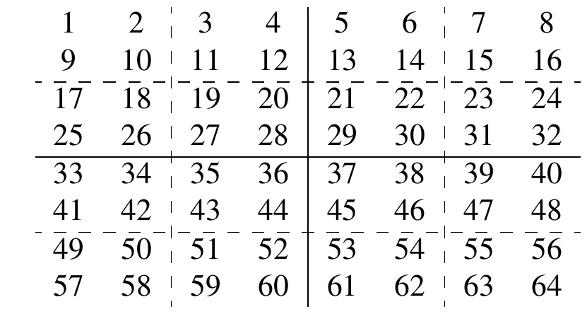
Now following the above discussed methodology, we have the following set of 6 blocks:
(1, 2, 9, 10, 5, 6, 13, 14, 33, 34, 41, 42, 37, 38, 45, 46, 3, 4, 11, 12, 7, 8, 15, 16, 35, 36, 43, 44, 39, 40, 47, 48)
(1, 2, 9, 10, 5, 6, 13, 14, 33, 34, 41, 42, 37, 38, 45, 46, 17, 18, 25, 26, 21, 22, 29, 30, 49, 50, 57, 58, 53, 54, 61, 62)
(1, 2, 9, 10, 5, 6, 13, 14, 33, 34, 41, 42, 37, 38, 45, 46, 19, 20, 27, 28, 23, 24, 31, 32, 51, 52, 59, 60, 55, 56, 63, 64)
(3, 4, 11, 12, 7, 8, 15, 16, 35, 36, 43, 44, 39, 40, 47, 48, 19, 20, 27, 28, 23, 24, 31, 32, 51, 52, 59, 60, 55, 56, 63, 64)
(3, 4, 11, 12, 7, 8, 15, 16, 35, 36, 43, 44, 39, 40, 47, 48, 17, 18, 25, 26, 21, 22, 29, 30, 49, 50, 57, 58, 53, 54, 61, 62)
(17, 18, 25, 26, 21, 22, 29, 30, 49, 50, 57, 58, 53, 54, 61, 62, 19, 20, 27, 28, 23, 24, 31, 32, 51, 52, 59, 60, 55, 56, 63, 64)
The above set of blocks constitutes a pseudo group divisible PBIB design with the following parameters: \[\begin{aligned} v&=64& b&=6 & r&=3 & k&=32\\ \lambda_1&=3& \lambda_2&=1 \end{aligned}\]
The parameters of the association scheme are: \[\begin{aligned} n_1&=15 & n_2&=48 \\ P_1&=\begin{bmatrix} 14&0\\ 0&48 \end{bmatrix} & P_2&=\begin{bmatrix} 0&15\\ 47&0 \end{bmatrix} \end{aligned}\]
The overall efficiency factor of the above constructed PBIB design is:
\[O_{eff} = 0.66 .\]
Our third series of PBIB designs is also obtained using property (iii) of magic squares. For this, we will construct a set of four blocks such that the \(i^{th}\) block (i = 1, 2, 3, 4) contains all the treatments except those which are contained in m\(\times\)m sub-squares denoted by integer i. Continuing in this way for all i = 1, 2, 3, 4; we will obtain a set of four blocks and this set of blocks constitutes a four-associate class PBIB design following Association scheme 4.3. The generalized parameters of such PBIB designs are: \[\begin{aligned} v&= M^2& b&=4 & r&=3 & k&=12m^2\\ \lambda_1&=3& \lambda_2&=\lambda_3=\lambda_4=2 \end{aligned}\]
As discussed earlier, a \(4\times4\) magic square can be partitioned into four \(2\times2\) sub-squares. Each of these \(2\times2\) sub-squares can be further partitioned into four \(1\times1\) sub-squares as shown below:
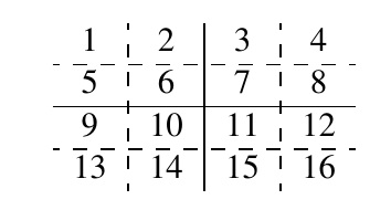
Now, following the above discussed methodology, we can form the following set of four blocks:
\[(2, 5, 6, 4, 7, 8, 10, 13, 14, 12, 15, 16)\] \[(1, 5, 6, 3, 7, 8, 9, 13, 14, 11, 15, 16)\] \[(1, 2, 6, 3, 4, 8, 9, 10, 14, 11, 12, 16)\] \[(1, 2, 5, 3, 4, 7, 9, 10, 13, 11, 12, 15)\]
The above set of blocks constitutes a four-associate class PBIB design with the following parameters: \[\begin{aligned} v&=16& b&=4 & r&=3& k&=12\\ \lambda_1&=3& \lambda_2&=\lambda_3=\lambda_4=2 \end{aligned}\]
The parameters of the association scheme are as given below: \[\begin{aligned} n_1&=3,\\ n_2&= n_3= n_4= 4,\\ P_1&=\begin{bmatrix} 2&0&0&0\\ 0&4&0&0\\ 0&0&4&0\\ 0&0&0&4 \end{bmatrix},\\ P_2&=\begin{bmatrix} 0&3&0&0\\ 3&0&0&0\\ 0&0&0&4\\ 0&0&4&0 \end{bmatrix},\\ P_3&=\begin{bmatrix} 0&0&3&0\\ 0&0&0&4\\ 3&0&0&0\\ 0&4&0&0 \end{bmatrix},\\ P_4&=\begin{bmatrix} 0&0&0&3\\ 0&0&4&0\\ 0&4&0&0\\ 3&0&0&0 \end{bmatrix}. \end{aligned}\]
The overall efficiency factor of the above constructed PBIB design is:
\[O_{eff} = 0.91 .\]
Our fourth series of PBIB designs is obtained by using both the properties (ii) and (iii) of magic squares. In this case, we will first select any of the four n\(\times\)n sub-squares and combine its treatments with the treatments contained in all the possible pairs of m\(\times\)m sub-squares belonging to the adjacent horizontally and vertically positioned n\(\times\)n sub-squares with respect to the selected n\(\times\)n sub-square. This procedure is repeated for all the four n\(\times\)n sub-squares and we will get a total of b = 48 blocks. This set of blocks will form a four-associate class PBIB design based on Association scheme 4.1 for a magic square of order \(2^2\times2^2\) and a five-associate class PBIB design based on Association scheme 4.4 for magic squares of order \(2^i\times2^i\) (i = 3, 4, …).
The parameters of the four-associate class PBIB design for case of magic square of order \(2^2\times2^2\) are given below: \[\begin{aligned} v&=16& b&=48 & r&=18 & k&=6\\ \lambda_1&=14 & \lambda_2&=\lambda_3=6& \lambda_4&=0 \end{aligned}\]
The parameters of the five-associate class PBIB design for case of magic square of order \(2^i\times2^i\) (i = 3, 4, …) are as given below: \[\begin{aligned} v&= M^2; where\ M= 2^i& b&=48 & r&=18& k&=6m^2\\ \lambda_1&=18& \lambda_2&=14& \lambda_3&=\lambda_4=6 & \lambda_5&=0 \end{aligned}\]
If we consider a \(4\times4\) magic square and follow the above discussed method, we can obtain the following set of blocks:
| (1, 2, 5, 6, 3, 4) | (1, 2, 5, 6, 3, 7) | (1, 2, 5, 6, 3, 8) |
| (1, 2, 5, 6, 4, 8) | (1, 2, 5, 6, 4, 7) | (1, 2, 5, 6, 7, 8) |
| (1, 2, 5, 6, 9, 10) | (1, 2, 5, 6, 9, 13) | (1, 2, 5, 6, 9, 14) |
| (1, 2, 5, 6, 10, 13) | (1, 2, 5, 6, 10, 14) | (1, 2, 5, 6, 13, 14) |
| (3, 4, 7, 8, 1, 2) | (3, 4, 7, 8, 5, 6) | (3, 4, 7, 8, 1, 5) |
| (3, 4, 7, 8, 2, 6) | (3, 4, 7, 8, 1, 6) | (3, 4, 7, 8, 2, 5) |
| (3, 4, 7, 8, 11, 12) | (3, 4, 7, 8, 15, 16) | (3, 4, 7, 8, 11, 15) |
| (3, 4, 7, 8, 12, 16) | (3, 4, 7, 8, 11, 16) | (3, 4, 7, 8, 12, 15) |
| (9, 10, 13, 14, 1, 2) | (9, 10, 13, 14, 5, 6) | (9, 10, 13, 14, 1, 5) |
| (9, 10, 13, 14, 2, 6) | (9, 10, 13, 14, 1, 6) | (9, 10, 13, 14, 2, 5) |
| (9, 10, 13, 14, 11, 12) | (9, 10, 13, 14, 15, 16) | (9, 10, 13, 14, 11, 15) |
| (9, 10, 13, 14, 12, 16) | (9, 10, 13, 14, 11, 16) | (9, 10, 13, 14, 12, 15) |
| (11, 12, 15, 16, 3, 4) | (11, 12, 15, 16, 7, 8) | (11, 12, 15, 16, 3, 7) |
| (11, 12, 15, 16, 4, 8) | (11, 12, 15, 16, 3, 8) | (11, 12, 15, 16, 4, 7) |
| (11, 12, 15, 16, 9, 10) | (11, 12, 15, 16, 13, 14) | (11, 12, 15, 16, 9, 13) |
| (11, 12, 15, 16, 10, 14) | (11, 12, 15, 16, 9, 14) | (11, 12, 15, 16, 10, 13) |
The above set of blocks constitutes a four-associate class PBIB design with the following parameters: \[\begin{aligned} v&=16& b&=48& r&=18 & k&=6\\ \lambda_1&=14& \lambda_2&=\lambda_3=6& \lambda_4&=0 \end{aligned}\] The parameters of the association scheme are same as those given in illustration 2. The overall efficiency factor of the above constructed PBIB design is:
\[O_{eff} = 0.49.\]
To explore the usefulness of magic squares in the construction of PBIB designs, we have first introduced a new method for the construction of magic squares and discussed their properties. We have then used these properties and proposed some new association schemes. The closeness of some of the properties of magic squares with some already existing association schemes is also discussed. Later in Section 5, these properties have been used to construct some series of PBIB designs based on the newly proposed association schemes.
The authors are highly thankful to the reviewers for their valuable suggestions and additions which made the paper more presentable.
| S. No. | v | b | r | k | \(\lambda_i\) | Overall efficiency (\( O_eff\)) | Obtained from |
| 1 | 16 | 4 | 2 | 8 | \(\lambda_1=2, \lambda_2=\lambda_3=1, \lambda_4=0\) | 0.60 | Series 1 |
| 2 | 64 | 4 | 2 | 32 | \(\lambda_1=2,\lambda_2=\lambda_3=1,\lambda_4=0\) | 0.62 | Series 1 |
| 3 | 16 | 6 | 3 | 8 | \(\lambda_1=3,\lambda_2=1\) | 0.64 | Series 2 |
| 4 | 64 | 6 | 3 | 32 | \(\lambda_1=3,\lambda_2=1\) | 0.66 | Series 2 |
| 5 | 16 | 4 | 3 | 12 | \(\lambda_1=3,\lambda_2=\lambda_3=\lambda_4=2\) | 0.91 | Series 3 |
| 6 | 64 | 4 | 3 | 48 | \(\lambda_1=3,\lambda_2=\lambda_3=\lambda_4=2\) | 0.92 | Series 3 |
| 7 | 16 | 48 | 18 | 6 | \(\lambda_1=14,\lambda_2=\lambda_3=6,\lambda_4=0\) | 0.49 | Series 4 |
| 8 | 64 | 48 | 18 | 24 | \(\lambda_1=18,\lambda_2=14, \lambda_3=\lambda_4=6,\lambda_5=0\) | 0.51 | Series 4 |