
Let \(G\) and \(H\) be graphs. Then \(G\) is said to have an \(H\)-covering if there exists a set \(\mathcal{H}=\{H_1,H_2,\dots,H_s\}\) of subgraphs of \(G\), all isomorphic to \(H\), such that every edge of \(G\) is contained in at least one graph in \(\mathcal{H}\). Also, \(G\) is said to have an \(H\)-decomposition if every edge of \(G\) is contained in exactly one graph in \(\mathcal{H}\). Therefore, every \(H\)-decomposition is also an \(H\)-covering, but the converse is not always true. The set \(\mathcal{H}\) is called a maximal \(H\)-covering if it contains all subgraphs of \(G\) isomorphic to \(H\).
Suppose \(G(V,E)\) is a graph with an \(H\)-covering. Then a function \(f\) from \(V\cup E\) to the set of integers \(\{1,2,\dots, |V|+|E|\}\) is called an \(H\)-magic labeling of \(G\) if there exists a positive integer \(\mu\) such that for every subgraph \(H_i\) of \(G\) with the vertex set \(V_i\) and edge set \(E_i\) the sum \(w(H_i)\) (called the weight of \(H_i\)) satisfies
\[w(H_i) = \sum_{x\in V_i} f(x) + \sum_{e\in E_i} f(e) = \mu.\]
The graph \(G\) is then called an \(H\)-magic graph. If \(f(V)\), the set of labels of all vertices of \(V\), is moreover equal to \(\{1,2,\dots,|V|\}\), then \(f\) is called an \(H\)-supermagic labeling of \(G\) (or \(H\)-SML for short) and \(G\) is an \(H\)-supermagic graph.
Similarly, when \(\mathcal{H}\) is an \(H\)-decomposition of \(G\) and the function \(f\) described above exists (that is, \(f\) is an \(H\)-SML), then \(\mathcal{H}\) is called an \(H\)-magic or \(H\)-supermagic decomposition of \(G\).
The notions of \(H\)-magic and \(H\)-supermagic labelings were introduced by Gutiérrez and Lladó [3] in 2005. While some \(H\)-magic decompositions appeared in various papers when the unique \(H\)-cover of some graph \(G\) was in fact a decomposition, the notion itself was first time formalized by Inayah, Lladó, and Moragas [4] in 2012.
There are many papers dealing with \(C_m\)-magic and supermagic labelings. We are not going to list them here; instead we refer the reader to section 5.4 in an excellent survey by Gallian [2].
Pradipta and Salman [10] defined a calendula graph \(Cal_{m,n}\) as the graph arising from the cycle \(C_m\) with vertices \(x_1,x_2,\dots,x_m\) and edges \(e_i=x_i x_{i+1}\) by joining \(x_i\) to \(x_{i+1}\) by a path \(P^i_{n}\). This way, we obtain a cycle of length \(n\) sharing the edge \(e_i\) with the cycle \(C_m\). Pradipta and Salman [10] proved that calendula graphs are \(C_n\)-supermagic for all \(m,n\geq3\). Öner and Ateş [7] proved the same result, using a different technique. Freyberg, Jensen and Scot [1] studied other types of magic labelings of calendula graphs.
We generalize the notion by defining rich calendula graphs or \(p\)-calendula graphs \(Cal_{m,p[n]}\) in a similar way, joining the vertices \(x_i\) and \(x_{i+1}\) by \(p\) internally disjoint paths \(P^{i,k}_n\). Because the distinction between the original calendula graphs and \(p\)-calendula graphs is clear from our notation, from now on we will only use the term calendula or rich calendula graph. Detailed notation will be provided in later sections.
We first present new constructions for calendula graphs \(Cal_{m,n}\) for any \(m,n\geq3\) and then prove that a \(C_n\)-supermagic labeling exists for \(p\)-calendula graphs \(Cal_{m,p[n]}\) for any \(m,n\geq3, \ p>1\) and \(m\neq n\). The case of \(m=n\) for \(p>1\) remains open.
We will denote by \([a,b]\) the set of integers \(\{a,a+1,\dots,b\}\) and when \(a=0\), we sometimes use just \([b]\) instead of \([1,b]\).
Pradipta and Salman [10] used for their labeling partitions of the multiset \([1,m]\cup[1,m(2n-1)]\) into \(m\) multisets with the same sum, each of them containing an element from \([1,m]\).
We use a different approach. The main idea is the following: we utilize the well-known fact that odd cycles are \(K_2\)-supermagic, and for even \(m=2t\) (where such labeling does not exist) we find a labeling in which either all copies of \(K_2\) but one have the same weights, or \(t\) of the \(K_2\)’s have one weight \(w'\) and the other \(t\) have weight \(w''\).
Then we use some modifications of \((2n-3)\times pm\) Kotzig arrays to label the remaining vertices and edges. An \(a\times b\) Kotzig array \({\mathrm{KA}}(a,b)\) consists of \(a\) rows, each containing a permutation of \([1,b]\) so that the sum of every column is equal to \(a(b+1)/2\). A \({\mathrm{KA}}(a,b)\) exists if and only if \(a\) is even, or \(ab\) is odd. For the case when \(a\) is odd and \(b\) is even, we use a similar array with two different column sums.
The structure of the paper is as follows. In Section 2, we provide a rigorous definition of rich calendula graphs and list some known related results. In Section 3, we present tools used in our constructions, namely Kotzig arrays and their modifications, and show some examples that will be the basic building blocks of our constructions. In Section 4, we provide \(C_n\)-supermagic labelings of simple calendula graphs \(Cal_{m,n}\) for all \(m,n\geq3\). In Section 5, we provide \(C_n\)-supermagic labelings of \(p\)-calendula graphs \(Cal_{m,p[n]}\) for all \(m,n\geq3, \ m\neq n\) and \(p>1\). In Section 6, we summarize our results and state an open problem for the case when \(m=n\) and \(p>1\).
First, we formally define rich calendula graphs.
Definition 2.1. A \(p\)-calendula graph \(Cal_{m,p[n]}\) consists of a central cycle \(C_m\) with vertices \(x_i, i\in[m]\) and \(pm\) petal cycles \(C^{i,k}_n, i\in[m], k\in[p]\) with vertices \(x^{i,k}_j,j\in[n]\) where \(x^{i,k}_1=x_i, x^{i,k}_n=x_{i+1}\) and all vertices \(x^{i,k}_j, i\in[m],k\in[p],j\in[2,n-1]\) are mutually distinct. When \(p=1\), we call the graph just a calendula graph and denote it \(Cal_{m,n}\).
Pradipta and Salman [10] and Öner and Ateş [7], using different techniques, proved independently the following.
Öner, Hussain and Banaras [9] and Öner and Erol [8] defined classes of graphs similar to calendula and rich calendula graphs, respectively, where the central cycle is replaced by a path. They called them polygonal snakes and book-snake graphs. That is, splitting one vertex of the central cycle of a calendula graph \(Cal_{m,n}\) into two gives a polygonal snake, and the same operation performed on a rich calendula graph gives a book-snake graph.
For the sake of exactness, we provide a formal definition.
Definition 2.3. A book-snake graph \(S(n,p,m)\) consists of a path \(P_{m+1}\) with vertices \(x_i, i\in[m+1]\) and \(pm\) cycles \(C^{i,k}_n, i\in[m], k\in[p]\) with vertices \(x^{i,k}_j,j\in[n]\) where \(x^{i,k}_1=x_i, x^{i,k}_n=x_{i+1}\) and all vertices \(x^{i,k}_j, i\in[m],k\in[p],j\in[2,n-1]\) are mutually distinct. When \(p=1\), we call the graph a polygonal snake and denote it \(\Delta^{n}_{m}\).
Öner, Hussain and Banaras [9] proved the following.
Theorem 2.4([9]).A polygonal snake \(\Delta^{n}_{m}\) is \(C_n\)-supermagic for every \(m,n\geq3\).
Öner and Erol [8] generalized the result as follows.
Theorem 2.5(8).A book-snake graph \(S(n,p,m)\) is \(C_n\)-supermagic for every \(m,n\geq3\).
We will generalize Theorem 2.2 in the same way Theorem 2.5 generalizes Theorem 2.4. That is, we amalgamate \(p\) cycles \(C_n\) to each edge of the central cycle \(C_m\).
In this section, we define Kotzig arrays as well as some of their modifications that will later be used in our constructions. Kotzig arrays were formally defined by Marr and Wallis [6] and named after Anton Kotzig, who used same cases in his paper [5]. We in fact use Kotzig’s original \(3\times b\) array in Example 3.6.
Definition 3.1. A Kotzig array \({\mathrm{KA}}(a,b)\) is an \(a\times b\) array with entries \(d_{i,j}\in\{1,2,\dots,b\}, 1\leq i\leq a, 1\leq j\leq b\) such that every row contains each number \(1,2,\dots,b\) exactly once, and the sum of every column is equal to the same constant \(\kappa(a,b)=a(b+1)/2\).
Theorem 3.2. There exists a \({\mathrm{KA}}(a,b)\) if and only if \(a>1\) and either \(a\) is even or \(a\) and \(b\) are both odd.
There are many different constructions of Kotzig arrays. We will rely on the following.
Construction 3.3. Let \(a=2s\). Define \({\mathrm{KA}}(a,b)=\{k_{i,j}\}\) for \(i=1,2,\dots,a\) and \(j=1,2,\dots,b\) by \[k_{i,j}= \begin{cases} j & \text{for} \ i \ \text{odd},\\ b+1-j \ &\text{for} \ i \ \text{even}. \end{cases}\]
Example 3.4. Let \(a=2\) and \(b=5\). Then \[{\mathrm{KA}}(2,5)= \begin{array}{|c|c|c|c|c|} \hline 1&2&3&4&5\\ \hline 5&4&3&2&1\\ \hline \end{array}\] with the column sums equal to 6 and for \(a=4\) and \(b=6\), \[{\mathrm{KA}}(4,6)= \begin{array}{|c|c|c|c|c|c|} \hline 1&2&3&4&5&6\\ \hline 6&5&4&3&2&1\\ \hline 1&2&3&4&5&6\\ \hline 6&5&4&3&2&1\\ \hline \end{array}\] with the column sums equal to 14.
Construction 3.5(Kotzig [5]).Let \(a=3\) and \(b=2t+1\). Define \({\mathrm{KA}}(3,b)=\{k_{i,j}\}\) for \(i=1,2,3\) and \(j=1,2,\dots,b\) as \[\begin{aligned} k_{1,j} &= b+1 – 2j, \\ k_{2,j} &= j + t + 1, \ \text{and}\\ k_{3,j} &= j, \end{aligned}\] where the calculations are performed modulo \(b\) with 0 replaced by \(b\).
Example 3.6(Kotzig [5]).Let \(a=3\) and \(b=2t+1=7\). Then \[{\mathrm{KA}}(3,7)= \begin{array}{|c|c|c|c|c|c|c|} \hline 6&4&2&7&5&3&1\\ \hline 5&6&7&1&2&3&4\\ \hline 1&2&3&4&5&6&7\\ \hline \end{array}\] and the column sums are all equal to 12.
It is easy to observe that for any odd \(a\geq5\) and odd \(b\) we can combine the two previous constructions to obtain a \({\mathrm{KA}}(a,b)\). We construct the first \(a-3\) rows as in Construction 3.3 and then add the rows of \({\mathrm{KA}}(3,b)\) from Construction 3.5.
In our labelings, we will use a modification of Kotzig arrays.
Definition 3.7. A \(c\)-lifted Kotzig array (or just lifted Kotzig array) \({\mathrm{LKA}}(a,b;c)\) arises from a \({\mathrm{KA}}(a,b)\) by increasing all elements in row \(i\) by \(c + (i-1)b\). That is, if \(K=\{k_{i,j}\}\) is a \({\mathrm{KA}}(a,b)\), then a \(c\)-lifted Kotzig array \(L=\{l_{i,j}\}\) is defined as \[l_{i,j} = k_{i,j} +(i-1)b+c.\]
Notice that a \({\mathrm{LKA}}(a,b;c)\) exists whenever a \({\mathrm{KA}}(a,b)\) exists, and the sum of every column is then \[\lambda(a,b;c) = a(b+1)/2 + ac + (a-1)ab/2 = a(c+(ab+1)/2).\]
We present two examples for the readers convenience.
Example 3.8. Let \(a=4,b=6\) and \(c=2\), then \[{\mathrm{LKA}}(4,6;2)= \begin{array}{|c|c|c|c|c|c|} \hline 3&4&5&6&7&8\\ \hline 14&13&12&11&10&9\\ \hline 15&16&17&18&19&20\\ \hline 26&25&24&23&22&21\\ \hline \end{array}\] with the column sums equal to 58 for \(a=5,b=7\) and \(c=3\) we have \[{\mathrm{LKA}}(5,7;3)= \begin{array}{|c|c|c|c|c|c|c|} \hline 4&5&6&7&8&9&10\\ \hline 17&16&15&14&13&12&11\\ \hline 23&21&19&24&22&20&18\\ \hline 29&30&31&25&26&27&28\\ \hline 32&33&34&35&36&37&38\\ \hline \end{array}\] with all column sums equal to 105.
The following is implied directly by the definition.
Theorem 3.9. A \(c\)-lifted Kotzig array \({\mathrm{LKA}}(a,b;c)\) exists whenever a Kotzig array \({\mathrm{KA}}(a,b)\) exists.
For our constructions, we will also need an array similar to \({\mathrm{LKA}}(a,b;c)\) in which all but one column sums are equal, while the last one is different.
Definition 3.10. A dented \(c\)-lifted Kotzig array (or just dented lifted Kotzig array) \({\mathrm{DLKA}}(a,b;c)\) is an \(a\times b\) array \(D=\{d_{i,j}\}\) \(i\in[1,a],j\in[1,b]\) where the set of entries in row \(i\) is equal to \([c+(i-1)b+1,c+ib]\), the sum of columns \(1,2,\dots,b-1\) is equal to the same constant \(\delta(a,b;c)\) and the sum of column \(b\) is equal to a different constant \(\delta^*(a,b;c)\).
We present an example of such an array for \(a\) odd and \(b\) even, which we will later use for our construction for \(m\) even and \(p=1\).
Construction 3.11. Set \(a=2s+3, b=2t\) and define first \(a-3\) rows as in an \({\mathrm{LKA}}(a,b;c)\); that is, \[d_{i,j}= \begin{cases} c+ (i-1)b+j \ &\text{for} \ i \ \text{odd},\\ c+ (i+1)b+1-j \ &\text{for} \ i \ \text{even}. \end{cases}\] The last three rows are defined as \[\begin{aligned} {7} &d_{a-2,j} &&= \begin{cases} c + (a-2)b +2 -2j &\text{for} \ \hskip15pt 1\leq j\leq t,\\ c + (a-2)b +1 -2(j-t) & \text{for} \ t+1 \leq j\leq 2t,\\ \end{cases} \\ &d_{a-1,j} &&= \begin{cases} c + (a-2)b +t +j & \text{for} \ \hskip16pt 1\leq j\leq t,\\ c + (a-2)b -t +j+1 & \text{for} \ t+1 \leq j\leq 2t-1,\\ c + (a-2)b +1 & \text{for} \hskip36pt j=2t,\\ \end{cases} \\ &d_{a,j} &&= \hskip9pt c+ (a-1)b + j. \end{aligned}\]
For instance, for \(a=5,b=8,c=3\) we have \[{\mathrm{DLKA}}(5,8;3)= \begin{array}{|c|c|c|c|c|c|c|c|} \hline 4&5&6&7&8&9&10&11\\ \hline 19&18&17&16&15&14&13&12\\ \hline 27&25&23&21&26&24&22&20\\ \hline 32&33&34&35&29&30&31&28\\ \hline 36&37&38&39&40&41&42&43\\ \hline \end{array}\] and the first seven columns add up to 118, while the last column sum is 114.
We first calculate \(\tilde{\delta}(a-3,b;c)\), the sum of entries in the first \(a-3\) rows for every \(1\leq j\leq b\). We start with adding two consecutive terms, \(d_{i,j}\) and \(d_{i+1,j}\) for \(i\) odd: \[\begin{aligned} {3} d_{i,j}+d_{i+1,j} &= \Big(c+(i-1)b + j\Big) &+ \Big(c+(i+2)b + 1 – j\Big)\\ &= 2c + (2i+1)b + 1. \end{aligned}\]
Then \[\begin{aligned} {5} \tilde{\delta}(a-3,b;c) &= \sum_{i \ \text{odd}, \ i=1}^{2s-1} 2c + (2i+1)b + 1 \\ &= s(2c + b + 1) + 2b \sum_{i \ \text{odd}, \ i=1}^{2s-1} i \\ &= s(2c+b+1)+2bs^2. \\ \end{aligned}\]
Now for \(1\leq j\leq t\), \[\begin{aligned} {3} d_{a-2,j}+d_{a-1,j} &= \Big(c+(a-2)b+2-2j\Big) + \Big(c+(a-2)b+t+j\Big)\\ &= 2c + (2a-4)b+t-j+2 , \end{aligned}\] and similarly for \(t+1\leq j\leq 2t-1\), \[\begin{aligned} {3} d_{a-2,j}+d_{a-1,j} &= \Big(c+(a-2)b+1-2(j-t)\Big) + \Big(c+(a-2)b+j-t+1\Big)\\ &= 2c + (2a-4)b+t-j+2. \end{aligned}\]
Therefore, for all \(1\leq j \leq b-1\), \[\begin{aligned} {5} {\delta}(a,b;c) &= \tilde{\delta}(a-3,b;c) + d_{a-2,j}+d_{a-1,j}+d_{a,j} \\ &= s(2c+b+1)+2bs^2 +\Big(2c + (2a-4)b+t-j+2\Big) +\Big(c+ (a-1)b + j\Big) \\ &= (2s+3)c + (2s^2 + s + 3a – 5)b + s + t + 2\\ &= ac + (s(a-2) + 3a – 5)b + s + t + 2. \end{aligned}\]
For \(j=b\), we have \[\begin{aligned} {3} d_{a-2,b}+d_{a-1,b} &= \Big(c+(a-2)b+1-2(b-t)\Big) + \Big(c+(a-2)b+1\Big)\\ &= \Big(c+(a-2)b+1-b\Big) + \Big(c+(a-2)b+1\Big)\\ &= 2c + (2a-5)b+2, \end{aligned}\] and \[\begin{aligned} {5} {\delta^*}(a,b;c) &= \tilde{\delta}(a-3,b;c) + d_{a-2,b}+d_{a-1,b}+d_{a,b} \\ &= s(2c+b+1)+2bs^2 +\Big(2c + (2a-5)b+2\Big) +\Big(c+ (a-1)b + b\Big) \\ &= (2s+3)c + (2s^2 + s + 3a – 5)b + s + 2\\ &= ac + (s(a-2) + 3a – 5)b + s + 2. \end{aligned}\]
As we know from Theorem 3.2, an \(a\times b\) Kotzig array with \(a\) odd only exists when \(b\) is odd. When \(b\) is even, we can construct a similar array where one half of the column sums differs from the other half by exactly one.
Defintion 3.12. A nearly-Kotzig array \({\mathrm{NKA}}(a,b)\), where \(a\) is odd and \(b=2t\) is even, is an \(a\times b\) array with entries \(d_{i,j}\in\{1,2,\dots,b\}, 1\leq i\leq a, 1\leq j\leq b\) such that every row contains each number \(1,2,\dots,b\) exactly once and the sum of entries in each of the first \(t\) columns is equal to the same constant \(\kappa_{F}(a,b)=\lceil a(b+1)/2\rceil\) while the sum entries in each of the last \(t\) columns is equal to the same constant \(\kappa_{L}(a,b)=\lfloor a(b+1)/2\rfloor\).
We construct one such \({\mathrm{NKA}}(a,b)\) now. We start with \({\mathrm{NKA}}(3,b)\).
Example 3.13. Let \(a=3\) and \(b=2t\). Define \(K=\{k_{i,j}\}\) for \(i=1,2,3\) and \(j=1,2,\dots,b\) by \[\begin{aligned} k_{1,j} &= \begin{cases} b+2 – 2j & \text{for }\ \ 1\leq j\leq t, \\ b+1 – 2(j-t)& \text{for \ } t+1\leq j\leq 2t, \end{cases} \\ k_{2,j} &= j + t, \end{aligned}\] and \(k_{3,j} = j,\) where the calculations are performed modulo \(b\) with 0 replaced by \(b\).
For instance, for \(b=8\) we have \[{\mathrm{NKA}}(3,8)= \begin{array}{|c|c|c|c|c|c|c|c|} \hline 8&6&4&2&7&5&3&1\\ \hline 5&6&7&8&1&2&3&4\\ \hline 1&2&3&4&5&6&7&8\\ \hline \end{array}\] with the first four column sums equal to 14 and the other four equal to 13.
Then it is easy to prove the following.
Theorem 3.14. There exists an \({\mathrm{NKA}}(a,b)\) whenever \(a>1\) is odd and \(b\geq2\) is even.
Proof. Combine \({\mathrm{KA}}(a-3,b)\) from Construction 3.3 with \({\mathrm{NKA}}(3,b)\) from Example 3.13. ◻
We can again define a lifted version of \({\mathrm{NKA}}\) as follows.
Definition 3.15. A \(c\)-lifted nearly-Kotzig array (or just lifted nearly-Kotzig array) \({\mathrm{LNKA}}(a,b;c)\) arises from a \({\mathrm{NKA}}(a,b)\) by increasing all elements in row \(i\) by \(c + (i-1)b\). That is, if \(K=\{k_{i,j}\}\) is an \({\mathrm{NKA}}(a,b)\), then a \(c\)-lifted nearly-Kotzig array \(L=\{l_{i,j}\}\) is defined as \[l_{i,j} = k_{i,j} +(i-1)b+c.\]
The following is implied directly by the definition.
Theorem 3.16. A \(c\)-lifted nearly-Kotzig array \({\mathrm{LNKA}}(a,b;c)\) exists for any \(a\geq3\) odd and \(b=2t\geq2\) even.
The column sum for the first and last \(t\) columns will be denoted by \(\lambda_{F}(a,b;c)\) and \(\lambda_{L}(a,b;c)\), respectively. We recall that \[\lambda_{F}(a,b;c) =\lambda_{L}(a,b;c)+1.\]
In this section, we deal with the (simple) calendula graphs \(Cal_{m,n}\) where to each edge of \(C_m\) we amalgamate a single copy of \(C_n\). While it was already shown in [10] that these graphs are \(C_n\)-supermagic for all \(m,n\geq3\), we present a different construction based on Kotzig arrays and their modifications. It is worth mentioning that because for \(p=1\) the cycles \(C_n\) decompose the calendula graph, one could also classify the labeling as a \(C_3\)-supermagic decomposition.
Throughout this whole section, we use the following notation and terminology.
The central cycle is the cycle \(C_m\) with vertices \(x_1,x_2,\dots,x_m\) and edges \(e_i=x_i x_{i+1}\). We also denote the graph \(K_2=\langle x_i, x_{i+1}\rangle\) as \(K^i\). The cycles \(C_n\), called petal cycles, will be denoted by \(C^{i}_n\) for \(i\in[1,m]\) with vertices \(x_i=x^{i}_{1},x^{i}_{2},x^{i}_{3},\dots,x^{i}_{n-1},x^{i}_{n}=x_{i+1}\) and edges \(e^{i}_u = x^{i}_u x^{i}_{u+1}\). We will call the sequence \(e^{i}_1,x^{i}_2,e^{i}_2,x^{i}_3,\dots,x^{i}_{n-1},e^{i}_{n-1}\) a quasi-path \({\tilde{P}}^{i}_n\). Then \(C^{i}_n = {\tilde{P}}^{i}_n \cup K^i\).
We start with the simplest case where \(m,n\) are both odd and distinct. We will use the fact that an odd cycle is \(K_2\)-supermagic and first find such a labeling. Then we replace the edge labels, originally in \([m+1,m]\) by the \(m\) largest labels in \([2m(n-2)+1,m(2n-1)]\). Then we arrange the remaining labels from \([m+1,2m(n-2)]\) in a \((2n-3)\times m\) \(m\)-lifted Kotzig array \({\mathrm{LKA}}(2n-3,m;m)\) and use each column for the unlabeled elements of one of the cycles \(C_n\). More precisely, we label with the \(j\)-th column the quasi-path \({\tilde{P}}^{i}_n\) so that the first (therefore lowest) \(n-2\) labels are assigned to vertices in any order, and the remaining \(m-1\) labels go to edges.
Construction 4.1. We first set \(m=2t+1\) and label the cycle \(C_m\) as follows: \[f(x_i) = (t(i+2)+2)\pmod{m} ,\] and \[f(e_i) =2m(n-1)+i.\]
Because the vertex labels are calculated modulo \(m\), finding the weight of \(K^i\) will be easier using the recursive definition of the labeling. We can see that \[\begin{aligned} f(x_{i+2}) &= t(i+4)+2 \pmod{m} \\ &= t(i+2)+2+2t \pmod{m} \\ &= f(x_i)+2t \pmod{m} \\ &= f(x_i)+m-1 \pmod{m} \\ &= f(x_i)-1 \pmod{m}. \end{aligned}\]
Also, \[\begin{aligned} f(e_{i+1}) &= 2m(n-1) + (i+1) \\ &= \big(2m(n-1) + i \big)+1 \\ &= f(e_i) +1. \end{aligned}\]
Then \[\begin{aligned} w(K^{i+1}) &= f(x_{i+1}) + f(x_{i+2})+ f(e_{i+1}) \\ &= f(x_{i+1}) + (f(x_{i})-1)+ (f(e_{i})+1)\\ &= f(x_{i}) + f(x_{i+1}) + f(e_{i}) +(-1+1) \\ &= w(K^i). \end{aligned}\]
To label the petal cycles \(C^{i}_n\), we will use the lifted Kotzig array \({\mathrm{LKA}}(2n-3,m;m)\). We label the elements of \({\tilde{P}}^{i}_n\) with the entries in column \(i\) so that vertices are labeled by entries in the first \(n-2\) rows followed by edge labels from the remaining \(n-1\) rows.
More precisely, we have for \(j=2,3,\dots,n-1\) (recall that \(x^{i}_1=x_i\) and \(x^{i}_m=x_{i+1}\) were already labeled in \(C_m\)) \[f(x^{i}_j) = l_{j-1,i},\] and for \(j=1,2,\dots,n-1\) \[f(e^{i}_j) = l_{n-2+j,i}.\]
Then, because the sum of entries in every column of \({\mathrm{LKA}}(2n-3,m;m)\) is equal to the same constant \(\lambda(2n-3,m;m)\), we have \[w(C^{i}_n) = w(K^i) + w({\tilde{P}}^{i}_n) =\mu(Cl_{m,n}) ,\] for every \(i\in[1,m]\) and \(f\) is a \(C_3\)-supermagic total labeling.
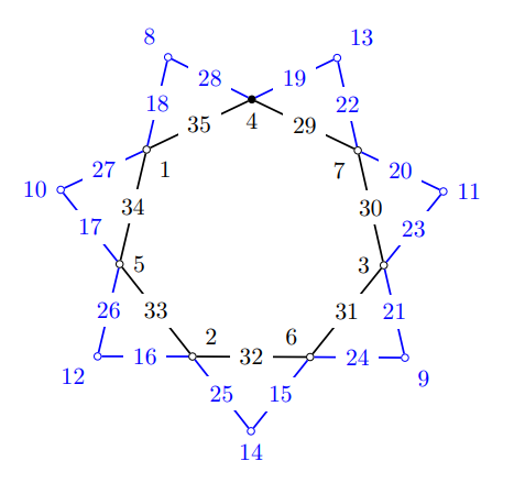
Example 4.2. We provide an example for \(m=7,n=3\). In Figure 1 the vertex \(x_1\) is solid and the subscripts increase going clockwise. The same convention will be used in all other examples. We always first present the relevant array with the column sums in the last row and then the labeled graph.
\[\begin{array}{|c|c|c|c|c|c|c|} \hline 13&11&9 &14&12&10&8 \\ \hline 19&20&21&15&16&17&18 \\ \hline 22&23&24&25&26&27&28 \\ \hline \hline 54&54&54&54&54&54&54\\ \hline \end{array}\] \[LKA(3,7;7)\]
Construction 4.1 proves the following theorem.
Theorem 4.3. Let \(m\) be odd, \(m,n\geq3\), and \(m\neq n\). Then the calendula graph \(Cal_{m,n}\) is \(C_n\)-supermagic.
In this case, we have to slightly modify our approach. There is no \(K_2\)-supermagic labeling of \(C_n\). Hence, we label the central cycle so that all \(K_2\) but one have the same weight \(w(K^i)=w(K^1)\) while the last one has the weight \(w(K^{m})=w(K^1) + m/2\). We again use the first \(m\) labels for vertices and the last \(m\) labels for edges. Then we use a dented \(m\)-lifted Kotzig array \({\mathrm{DLKA}}(2n-3,m;m)\) in which the sum of the last column is by \(m/2\) smaller than the other \(m-1\) column sums. This compensates the higher weight of the graph \(K^m\).
Construction 4.4. We set \(m=2t\) and label the cycle \(C_m\) as follows: \[f(x_i) = \begin{cases} t-(i-1)/2 & \text{for $i$ odd},\\ 2t+1 – i/2 & \text{for $i$ even}, \end{cases}\] and \(f(e_i) =2m(n-1)+i.\) Then for \(i=1,3,\dots,m-1\) \[\begin{aligned} w(K^{i}) &= f(x_{i}) + f(x_{i+1}) + f(e_{i}) \\ &= t-(i-1)/2 + 2t+1 – (i+1)/2 + 2m(n-1)+i \\ &= 3t +2m(n-1) + 1, \end{aligned}\] ad for \(i=2,4,\dots,m-2\) \[\begin{aligned} w(K^{i}) &= f(x_{i}) + f(x_{i+1}) + f(e_{i}) \\ &= 2t+1-i/2 + t – (i+1-1)/2 + 2m(n-1)+i \\ &= 3t + 2m(n-1) + 1. \end{aligned}\]
The only \(K^i\) with different weight is \(K^{m}\) where \[\begin{aligned} w(K^{m}) &= f(x_{m}) + f(x_{1}) + f(e_{m}) \\ &= 2t+1- m/2 + t – (1-1)/2 + 2m(n-1)+m \\ &= 2t+1- t + t + 2m(n-1)+2t \\ &= 4t +2m(n-1) + 1. \end{aligned}\]
It follows that \[w(K^{m}) = w(K^{1}) + t = w(K^{1}) +m/2.\]
To label the petal cycles \(C^{i}_n\), we will use the dented lifted Kotzig array \({\mathrm{DLKA}}(2n-3,m;m)\) constructed in Construction 3.11. We label the elements of \({\tilde{P}}^{i}_n\) with the entries in column \(i\). The vertices are labeled by entries in the first \(n-2\) rows while edges are labeled by the remaining \(n-1\) rows.
As in the previous construction, \(x^{i}_1=x_i\) and \(x^{i}_n=x_{i+1}\) were already labeled in \(C_m\). Therefore, for \(j=2,3,\dots,n-1\) we have \(f(x^{i}_j) = l_{j-1,i},\) and for \(j=1,2,\dots,n-1\) \(f(e^{i}_j) = l_{n-2+j,i}.\)
We have shown in Construction 3.11 that \[\begin{aligned} {5} {\delta}(a,b;c) &= ac + (s(a-2) + 3a – 5)b + s + t + 2, \end{aligned}\] and \[\begin{aligned} {5} {\delta^*}(a,b;c) &= ac + (s(a-2) + 3a – 5)b + s + 2. \end{aligned}\]
Therefore, \({\delta^*}(a,b;c) = {\delta}(a,b;c) – t,\) which for \(a=2n-3, b=m, c=m\) yields \[\begin{aligned} {5} {\delta^*}(2n-3,m;m) &= {\delta}(2n-3,m;m) – m/2. \end{aligned}\]
In terms of graph weights we have \(w({\tilde{P}}^{m}_n) = w({\tilde{P}}^{1}_n) – m/2.\) Now for every \(i\in[1,m-1]\) \(w(C^{i}_n) = w(K^i) + w({\tilde{P}}^{i}_n),\) and for \(i=m\) \[\begin{aligned} w(C^{m}_n) &= w(K^m) + w({\tilde{P}}^{m}_n) = w(K^1) + m/2 \ \ + w({\tilde{P}}^{1}_n) – m/2 = w(K^1) + w({\tilde{P}}^{1}_n). \end{aligned}\]
Therefore, the weight of every cycle \(C^i_n\), \(i\in[1,m]\) is the same and \(f\) is a \(C_n\)-supermagic labeling.
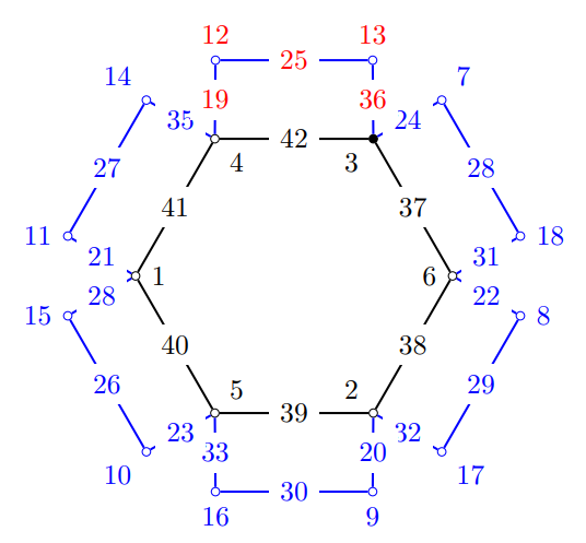
Example 4.5. In this example for \(m=6,n=4\) the last column with the smaller sum and the corresponding labels in Figure 2 are in red.
| 7 | 8 | 9 | 10 | 11 | 12 |
| 18 | 17 | 16 | 15 | 14 | 13 |
| 24 | 22 | 20 | 23 | 21 | 19 |
| 28 | 29 | 30 | 26 | 27 | 25 |
| 31 | 32 | 33 | 34 | 35 | 36 |
| 108 | 108 | 108 | 108 | 108 | 105 |
\[DLKA(5,6;6)\]
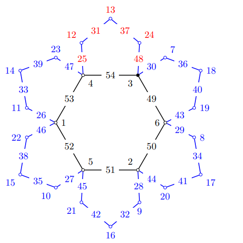
Example 4.6. As in the previous example, here for \(m=6,n=5\) the last column with the smaller sum and the corresponding labels in Figure 3 are in red.
| 7 | 8 | 9 | 10 | 11 | 12 |
| 18 | 17 | 16 | 15 | 14 | 13 |
| 19 | 20 | 21 | 22 | 23 | 24 |
| 30 | 29 | 28 | 27 | 26 | 25 |
| 36 | 34 | 32 | 35 | 33 | 31 |
| 40 | 41 | 42 | 38 | 39 | 37 |
| 43 | 44 | 45 | 46 | 47 | 48 |
| 193 | 193 | 193 | 193 | 193 | 190 |
\[DLKA(7,6;6)\]
Construction 4.4 proves the following.
Theorem 4.7. Let \(m\) be even, \(m\geq4,n\geq3\), and \(m\neq n\). Then the calendula graph \(Cal_{m,n}\) is \(C_n\)-supermagic.
For \(m=n\) we have one extra cycle \(C_n\) that needs to have the same weight as the remaining cycles. We denote the central cycle \(C^0_n\).
In Constructions 4.1 and 4.4 we have \[w(C^i_n) = 2n^3 – 2n^2 + 2n,\] and \[w(C^0_n) = 2n^3 – n^2 + n.\]
Therefore, \[w(C^0_n) – w(C^i_n) = (2n^3 – n^2 + n) – (2n^3 – 2n^2 + 2n) = n^2 – n.\]
To obtain a \(C_n\)-supermagic labeling, we need to decrease the weight of \(C^0_n\) by \(n^2-n\) without changing the weight of the petal cycles. This can be done by mutually swapping the labels between \(e_i\) and \(e^i_j\) for \(i\in[1,n-1]\) such that \[f(e_i) – f(e^i_j) = n.\]
Because \(e_i\) (which is actually equal to \(e^i_n\) using the notation within \(C^i_n\)) and \(e^i_j\) belong to the same petal cycle \(C^i_n\), the weight of \(C^i_n\) does not change, while the weight of \(C^0_n\) will decrease by \((n-1)n\).
We formalize the new labeling as follows.
Construction 4.8. Let \(f\) be the labeling function used in Constructions 4.1 and 4.4 for \(m\) odd and even, respectively.
We first recall that the edge \(e_i\) on the central \(C^0_n\) is denoted as \(e^i_n\) when considered on the petal cycle \(C^i_n\). Then \(f(e^i_{n-1}) = (2n-3)n + i,\) and \(f(e_i) = f(e^i_{n}) = (2n-2)n + i.\) Hence, \[f(e_i) – f(e^i_{n-1}) = (2n-2)n + i -((2n-3)n + i) = n.\]
Then we define a new labeling \(g\) as follows: \[\begin{aligned} &g(x_i) = f(x_i) \\ &g(x^i_j) = f(x^i_j) \\ &g(e_i) = f(e^i_{n-1}) & \text{for} \ i\in[1,n-1] \\ &g(e^i_{n-1}) = f(e_i) & \text{for} \ i\in[1,n-1] \\ &g(e_n) = f(e_n) \\ &g(e^i_{j}) = f(e^i_j) & \text{otherwise.} \end{aligned}\]
We now denote the weight functions for labelings \(f\) and \(g\) as \(w_f\) and \(w_g\), respectively. It should be obvious that for every \(i\in[1,n]\), \[w_g(C^i_n) = w_f(C^i_n),\] because the label swap between edges \(e_i\) and \(e^i_{n-1}\) was performed within the particular cycle \(C^i_n\). For the central cycle, we have \[\begin{aligned} {5} w_g(C^0_n) &= w_f(C^0_n) – \sum_{i=1}^{n-1} f(e_i) + \sum_{i=1}^{n-1} f(e^i_{n-1}) = w_f(C^0_n) – \sum_{i=1}^{n-1} \Big(f(e_i)- f(e^i_{n-1})\Big)\\ &= w_f(C^0_n) – \sum_{i=1}^{n-1} n = w_f(C^0_n) – (n-1)n = w_f(C^i_n), \end{aligned}\] for any \(i\neq0\), which implies that \(w_g(C^0_n) = w_g(C^i_n),\) for every \(i\in[1,n]\) and \(g\) is a \(C_n\)-supermagic labeling.
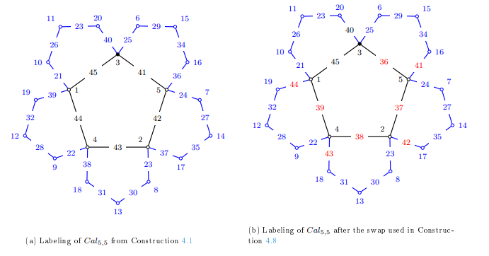
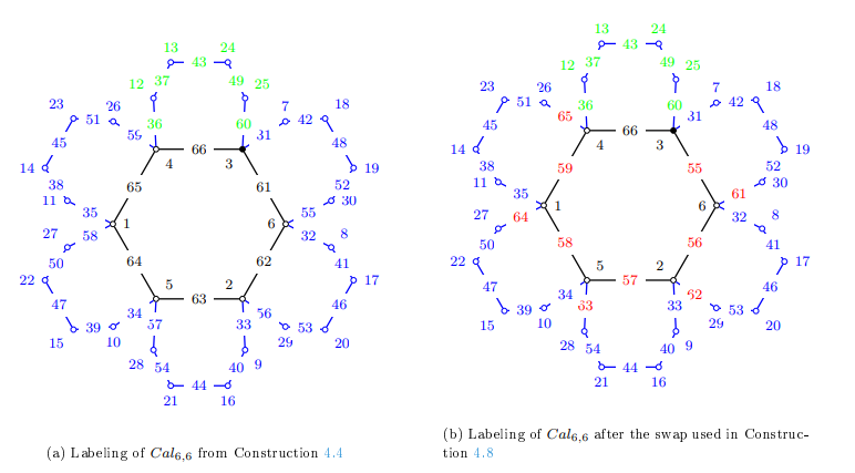
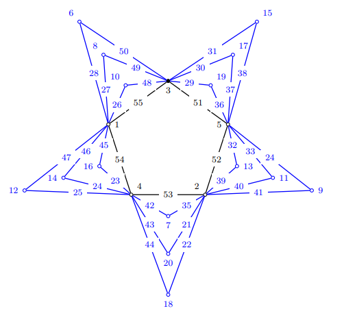
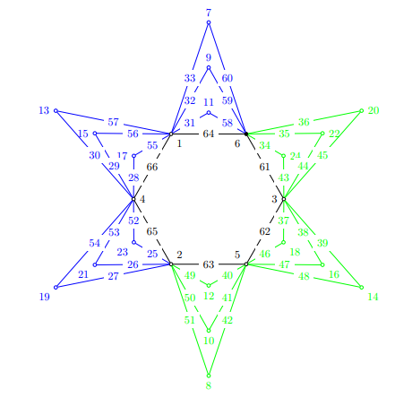
Example 4.9. In this example for \(n=5\) we first present in Figure 4 the labeling obtained by Construction 4.1 in which the central cycle has the weight \(w(C^0_n) = 2n^3 – n^2 + n=230\) and the petal cycles have \(w(C^i_n) = 2n^3 – 2n^2 + 2n=210\). Hence, their weights differ by \(n^2-n=20\). To eliminate the difference, we swap labels in cycles \(C^i_5\) for \(i\in[1,4]\) as shown in part (b) of Figure 4.
| 6 | 7 | 8 | 9 | 10 |
| 15 | 14 | 13 | 2 | 11 |
| 16 | 17 | 18 | 19 | 20 |
| 25 | 24 | 23 | 22 | 21 |
| 29 | 27 | 30 | 28 | 26 |
| 34 | 35 | 31 | 32 | 33 |
| 36 | 37 | 38 | 39 | 40 |
| 161 | 161 | 161 | 161 | 161 |
\[LKA(7,5;5)\]
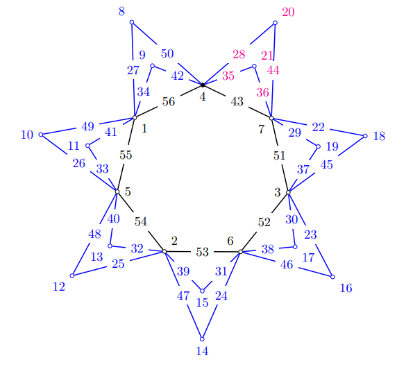
Example 4.10. In this example for \(n=6\) we first present in Figure 5 part (a) the labeling obtained by Construction 4.4 and highlight in green the labels corresponding to the last column of the dented array \(DLKA(9,6;6)\) with the smaller sum.
The edge label swap is done in part (b) as in the previous example and highlighted in red.
| 7 | 8 | 9 | 10 | 11 | 12 |
| 18 | 17 | 16 | 15 | 14 | 13 |
| 19 | 20 | 21 | 22 | 23 | 24 |
| 30 | 29 | 28 | 27 | 26 | 25 |
| 31 | 32 | 33 | 34 | 35 | 36 |
| 37 | 38 | 37 | 40 | 41 | 42 |
| 48 | 46 | 44 | 47 | 45 | 43 |
| 52 | 53 | 54 | 50 | 51 | 49 |
| 55 | 56 | 57 | 58 | 59 | 60 |
| 155 | 155 | 155 | 155 | 155 | 152 |
\[DLKA(9,6;6)\]
Construction 4.8 proves the following.
Theorem 4.11. Let \(n\geq3\). Then the calendula graph \(Cal_{n,n}\) is \(C_n\)-supermagic.
When the first draft of this paper was written, the author was unaware of the previous results by Pradipta and Salman [10] and, similarly to them, was only focusing on the simple case for \(p=1\). This resulted in what is now presented in Section 4. After finding out that the case was already completely solved, the author was hesitant to waste his previous effort by abandoning the topic. Instead, he decided to generalize the results by introducing \(p\)-calendula graphs. It turned out that the methods used in Section 4 would resist generalization for \(mp\) even. Therefore, another modification of lifted Kotzig arrays was used and not too surprisingly, it worked for all positive values of \(p\), including \(p=1\). This might have made the previous constructions pointless.
The author nevertheless decided to keep the constructions in the paper with the hope that they may become useful in finding \(H\)-supermagic labelings of other graphs.
It is worth remarking here that we were unable to find a construction for the case when \(p>1\) and \(m=n\). Therefore, we leave it as an open problem that we will formally state at the end of this paper.
For \(mp\) odd and \(m\neq n\), the construction is very similar to Construction 4.1 because we again have an odd number of cycles \(C_n\).
Construction 5.1. We again set \(m=2t+1\) and label the cycle \(C_m\) similarly as in Construction 4.1, that is, \[f(x_i) = (t(i+2)+2)\pmod{m} ,\] and \[f(e_i) = m(2np – 3p + 1) + i.\]
We again find the weight of \(K^i\) using the recursive definition of the labeling. We can see that \[\begin{aligned} {7} f(x_{i+2}) &= t(i+4) +2 \pmod{m} \\ &= t(i+2) +2 + 2t \pmod{m} \\ &= f(x_i) +2t \pmod{m} \\ &= f(x_i) + m-1 \pmod{m} \\ &= f(x_i) -1 \pmod{m}. \end{aligned}\]
Also, \[\begin{aligned} f(e_{i+1}) &= m(2np – 3p + 1) + (i+1) \\ &= \big(m(2np – 3p + 1) + i \big)+1 \\ &= f(e_i) +1. \end{aligned}\]
Then, denoting \(\kappa= w(K_1)\), \[\begin{aligned} {6} w(K^{i+1}) &= f(x_{i+1}) + f(x_{i+2}) + f(e_{i+1}) \\ &= f(x_{i+1}) + (f(x_{i})-1)+ (f(e_{i})+1)\\ &= f(x_{i}) + f(x_{i+1}) + f(e_{i}) +(-1+1) \\ &= w(K^i) = \kappa, \end{aligned}\] for every \(i\in[1,m]\).
Next, we construct a \((2n-3)\times mp\) lifted Kotzig array \({\mathrm{LKA}}(2n-3,mp;m)\), which exists by Theorem 3.2 because \(mp\) odd implies \(m\) odd. Then we use the labels in column \(j=pq+r, \ 0\leq q\leq m-1, \ 1<r\leq p\) to label the quasi-path \({\tilde{P}}^{q+1,r}_n\) so that the first \(n-2\) rows label the vertices and the remaining \(n-1\) rows label the edges. Because the sum of entries in every column is equal to the same constant \(\lambda(2n-3,mp;m)\), we have \[w(C^{i,k}_n) = \lambda(2n-3,mp;m) + w(K^i) = \lambda(2n-3,mp;m) + \kappa,\] and the graph \(Cal_{m,p[n]}\) is \(C_n\)-supermagic.
Example 5.2. In this and following examples, the cycles \(C^{i,k}_n\) for \(k\in[1,p]\) are drawn from inner to outer as \(k\) increases. We show an example for \(m=5,n=3,p=3\).
| 19 | 17 | 15 | 13 | 11 | 9 | 7 | 20 | 18 | 16 | 14 | 12 | 10 | 8 | 6 |
| 29 | 30 | 31 | 32 | 33 | 34 | 35 | 21 | 22 | 23 | 24 | 25 | 26 | 27 | 28 |
| 36 | 37 | 38 | 39 | 40 | 41 | 42 | 43 | 44 | 45 | 46 | 47 | 48 | 49 | 50 |
| 84 | 84 | 84 | 84 | 84 | 84 | 84 | 84 | 84 | 84 | 84 | 84 | 84 | 84 | 84 |
\[LKA(3,15;5)\]
The theorem follows from Construction 5.1 immediately.
Theorem 5.3. Let \(m,p\) be odd, \(m,n\geq3\), \(p\geq 1\) and \(m\neq n\). Then the rich calendula graph \(Cal_{m,p[n]}\) is \(C_n\)-supermagic.
This is the most complicated case of this section. Although for \(m\) odd there exists a \(K_2\)-supermagic labeling of \(C_m\), we were unable to find a construction that would label the central cycle that way. Instead, we used a labeling similar to that in Construction 4.4 in which one \(K_2\) received a different weight. This is achieved by using for the edges on the central \(C_m\) non-consecutive labels, more specifically, we use labels in \(\{m(2pn-3p)+1\}\cup [m(2pn-3p+1)+2,m(2pn-3p+2)]\). This gives the graph \(K^1\) a weight that is by \(mp/2\) smaller than the weights of the remaining graphs \(K^i\).
Then we construct an \((2n-3)\times mp\) array \(Q\) based on a lifted nearly Kotzig array \({\mathrm{LNKA}}(2n-3,mp;m)\) in which we have \(p\) columns with a weight that differs from the other column weights by \(mp/2\). This array \(Q\) consists of non-consecutive numbers, with \(m(2pn-3p)+1\) (that is used for \(C_m\)) skipped.
Construcion 5.4. We first set \(m=2t+1, \ p=2s\) and label the cycle \(C_m\) as follows: \[f(x_i) = (ti+1)\pmod{m}\] and \[f(e_i) = \begin{cases} mp(2n-3)+i \hskip33pt \text{for $i=1$}\\ mp(2n-3)+i+ms \hskip8pt \text{for $2\leq i\leq m$.}\\ \end{cases}\]
The vertex labels are calculated modulo \(m\), hence finding the weight of \(K^i\) will be easier using recursive definition of the labeling. We can see that \[\begin{aligned} f(x_{i+2}) &= t(i+2) +1 \pmod{m} \\ &= ti +1 + 2t \pmod{m} \\ &= f(x_i) + 2t \pmod{m} \\ &= f(x_i) + m-1 \pmod{m} \\ &= f(x_i) -1 \pmod{m}. \end{aligned}\]
Also, for \(i\in[2,m-1]\) \[\begin{aligned} f(e_{i+1}) &= mp(2n-3)+(i+1)+ms \\ &= \big(mp(2n-3)+ i+ms \big)+1 \\ &= f(e_i) +1. \end{aligned}\]
Then we have \[\begin{aligned} w(K^{1}) &= f(x_{1}) + f(x_{1}) + f(e_{1}) \\ &= t\cdot1+1 + t\cdot2+1 + mp(2n-3)+1 \\ &= 3t +mp(2n-3)+ 3\\ &= mp(2n-3) + (2t+1) +(t+2)\\ &= mp(2n-3) + m +(t+2)\\ &= m(2np-3p+1) +(t+2), \end{aligned}\] and for \(i\in[2,m-1]\), \[\begin{aligned} w(K^{i+1}) &= f(x_{i+1}) + f(x_{i+2}) + f(e_{i+1}) \\ &= f(x_{i+1}) + (f(x_{i})-1)+ (f(e_{i})+1)\\ &= f(x_{i}) + f(x_{i+1}) + f(e_{i}) +(-1+1) \\ &= w(K^i). \end{aligned}\]
Now we recall that the vertex labels are calculated modulo \(m\) with 0 replaced by \(m\), hence \[f(x_2) = (t\cdot2+1)\pmod{m} = (2t+1)\pmod{m} = m\pmod{m} = m,\] and \[f(x_3) = (t\cdot3+1)\pmod{m} = (2t+1 +t)\pmod{m} = (m+t)\pmod{m} = t.\]
Then for every \(i\in[2,m]\) we have \[\begin{aligned} w(K^{i})=w(K^{2}) &= f(x_{2}) + f(x_{3}) + f(e_{2}) \\ &= m + t + mp(2n-3)+ms+2 \\ &= m + t + m(2np-3p)+ms+2 \\ &= m(2np-3p+1) +(t+2) +ms\\ &= w(K^1) +ms. \end{aligned}\]
This means that we now need to label the quasi-paths so that \[w({\tilde{P}}^{1,k}_{n}) = w({\tilde{P}}^{i,l}_{n}) – ms,\] for every \(i\in[2,m], \ k,l\in[1,p]\). It can be achieved by modifying the lifted nearly-Kotzig array \({\mathrm{LNKA}}(2n-3,mp;m)\).
Table 14\[LNKA(3,14;7)\]
We shift the entries in the second half of the last row by one to the left, that is, increasing each entry by one. Then we cyclically shift each half of the row \(2n-4\) by \(s\) positions to the right. For the reader’s convenience, we highlighted some of the affected entries.
| 21 | 19 | 17 | 15 | 13 | 11 | 9 | 20 | 18 | 16 | 14 | 12 | 10 | 8 |
|---|---|---|---|---|---|---|---|---|---|---|---|---|---|
| 35 | 29 | 30 | 31 | 32 | 33 | 34 | 28 | 22 | 23 | 24 | 25 | 26 | 27 |
| 36 | 37 | 38 | 39 | 40 | 41 | 42 | 44 | 45 | 46 | 47 | 48 | 49 | 50 |
| 92 | 85 | 85 | 85 | 85 | 85 | 85 | 92 | 85 | 85 | 85 | 85 | 85 | 85 |
\[\text{Modified\ } LNKA(3,14;7)\]
We now describe the process more formally. Let \(D=\{d_{i,j}\}, \ i\in[1,2n-3], \ j\in[1,mp]\) be an \({\mathrm{LNKA}}(2n-3,mp;m)\) with column sums \(\lambda_{F}(2n-3,mp;m)\) for the first \(ms\) columns and \(\lambda_{L}(2n-3,mp;m)=\lambda_{F}(2n-3,mp;m)-1\) for the last \(ms\) columns. We will call them just \(\lambda_{F}\) and \(\lambda_{L}\), respectively. Define an \((2n-3)\times mp\) array \(Q=\{q_{i,j}\}\) as \[\begin{aligned} q_{i,j} =& d_{i,j} \hskip120pt \text{for $i\in[1,2n-5],j\in[1,2ms]$,}\\ q_{2n-4,j} =& \begin{cases} d_{2n-4,j} + (m-1)s\qquad \hskip2pt \text{for $j\in[1,s]\cup[ms+1,(m+1)s]$}\\ d_{2n-4,j} – s\qquad \hskip42pt \text{for $j\in[s+1,ms]\cup[ms+s+1,2ms]$,} \end{cases}\\ q_{2n-3,j} =& \begin{cases} d_{2n-3,j} \qquad \hskip63pt \text{for $j\in[1,ms]$}\\ d_{2n-3,j} + 1\qquad \hskip44pt \text{for $j\in[ms+1,2ms]$}. \end{cases} \end{aligned}\]
Denote the column sum in column \(j\) by \(\sigma_j\). Then for \(j\in[1,s]\) \[\begin{aligned} {3} \sigma_j &= \lambda_{F} +(m-1)s= \lambda_{F} -s +ms, \end{aligned}\] for \(j\in[ms+1,(m+1)s]\) \[\begin{aligned} {3} \sigma_j &= \lambda_{L} + (m-1)s +1\\ &= \lambda_{F} -1 + (m-1)s +1\\ &= \lambda_{F} + (m-1)s \\ &= \lambda_{F} -s +ms, \end{aligned}\] for \(j\in[s+1,ms]\) \[\begin{aligned} {3} \sigma_j &= \lambda_{F} -s,\\ \end{aligned}\] and for \(j\in[ms+s+1,2ms]\) \[\begin{aligned} {3} \sigma_j &= \lambda_{L} -s +1= \lambda_{F} -1 -s +1= \lambda_{F} -s. \end{aligned}\]
We have \(2s=p\) columns with sum \(\lambda_{F}-s+ms\) and remaining \((m-1)p\) columns with sum \(\lambda_{F}-s\). We use the columns with the higher sum to label the quasi-paths \({\tilde{P}}^{1,k}_n\) for all \(k\in[1,p]\) and the remaining columns for the quasi-paths \({\tilde{P}}^{i,l}_{n}, \ i\in[2,m], \ l\in[1,p]\).
Then the cycle weights for \(i=1, \ k\in[1,p]\) are \[\begin{aligned} {3} w(C^{1,k}_n) &= w(K^1) +w({\tilde{P}}^{1,k}_{n})= w(K^1) +\lambda_{F} – s + ms, \end{aligned}\] and for \(i\in[2,m], \ l\in[1,p]\) they are \[\begin{aligned} {3} w(C^{i,l}_n) &= w(K^i) +w({\tilde{P}}^{1,l}_{n})\\ &= w(K^1)+ms +\lambda_{F} – s\\ &= w(K^1) +\lambda_{F} – s+ms\\ &=w(C^{1,k}_n). \end{aligned}\]
Therefore, all cycles \(C_n\) have the same weight and \(f\) is an \(H\)-supermagic labeling of \(Pl_{m,p[n]}\).
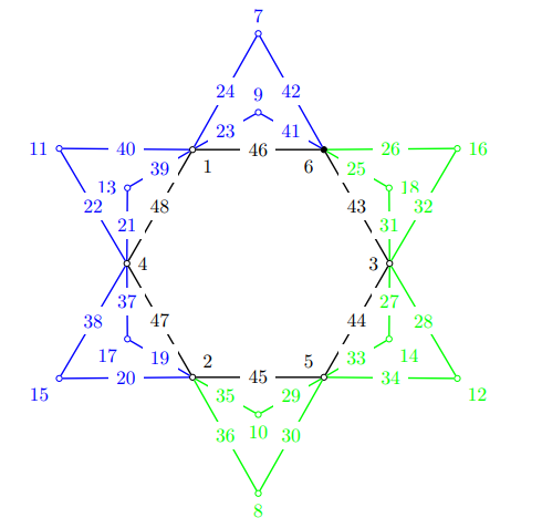
Example 5.5. In this example for \(m=7,n=3,p=2\) we highlight the two columns with different sums and the corresponding labels in Figure 7.
| 21 | 19 | 17 | 15 | 13 | 11 | 9 | 20 | 18 | 16 | 14 | 12 | 10 | 8 |
|---|---|---|---|---|---|---|---|---|---|---|---|---|---|
| 35 | 29 | 30 | 31 | 32 | 33 | 34 | 28 | 22 | 23 | 24 | 25 | 26 | 27 |
| 36 | 37 | 38 | 39 | 40 | 41 | 42 | 44 | 45 | 46 | 47 | 48 | 49 | 50 |
| 92 | 85 | 85 | 85 | 85 | 85 | 85 | 92 | 85 | 85 | 85 | 85 | 85 | 85 |
\[\text{Modified\ } LNKA(3,14;7)\]
Construction 5.4 yields our next theorem.
Theorem 5.6. Let \(m\geq3\) be odd, \(p\geq2\) even, \(n\geq3\), and \(m\neq n\). Then the rich calendula graph \(Cal_{m,p[n]}\) is \(C_n\)-supermagic.
As we mentioned before, there is no \(K_2\)-supermagic labeling of \(C_m\) for \(m\) even. However, we can label the vertices by \([1,m]\) and edges by \([m+1,2m]\) so that the there are exactly two different edge weights. More specifically, if \(m=2t\), then the weights of the last \(t\) edges will be bigger by one than the weights of the first \(t\) edges.
Then we label the remaining elements of the cycles \(C_n\) attached to the first \(t\) edges by the first \(tp\) columns of an \({\mathrm{NKA}}(2n-3,mp;p)\) and the cycles attached to the last \(t\) edges of \(C_m\) by the last \(tp\) columns.
Construction 5.7. We set \(m=2t\) and label the cycle \(C_m\) as follows: \[f(x_i) = \begin{cases} 2t – (i-1)/2 \hskip7pt \text{for $i$ odd},\\ t+1 – i/2 \hskip20pt \text{for $i$ even}, \end{cases}\] and \[f(e_i) = \begin{cases} m(2np-3p+1)+ i \hskip24pt \text{for $1\leq i\leq t$},\\ m(2np-3p+1)+i+1 \hskip7pt \text{for $t+1\leq i\leq 2t-1$},\\ m(2np-3p+1)+t+1 \hskip7pt \text{for $i=m$,} \end{cases}\] using the highest \(m\) labels.
Then for \(i\leq t\), \(i\) odd \[\begin{aligned} {5} w(K^{i}) &= f(x_{i}) + f(x_{i+1}) + f(e_{i}) \\ &= 2t-(i-1)/2 + t+1 – (i+1)/2 + m(2np-3p+1)+i \\ &= {3t +m(2np-3p+1) + 1}, \end{aligned}\] and for \(i\leq t\), \(i\) even \[\begin{aligned} {5} w(K^{i}) &= f(x_{i}) + f(x_{i+1}) + f(e_{i}) \\ &= t+1-i/2 + 2t – (i-2)/2 + m(2np-3p+1)+i \\ &={ 3t + m(2np-3p+1) + 1.} \end{aligned}\]
Also for \(t+1\leq i\leq 2t-1\), \(i\) odd \[\begin{aligned} {5} w(K^{i}) &= f(x_{i}) + f(x_{i+1}) + f(e_{i}) \\ &= 2t-(i-1)/2 + t+1 – (i+1)/2 + m(2np-3p+1)+i+1 \\ &= {3t +m(2np-3p+1) + 2}, \end{aligned}\] and for \(t=1\leq i\leq 2t-2\), \(i\) even \[\begin{aligned} {5} w(K^{i}) &= f(x_{i}) + f(x_{i+1}) + f(e_{i}) \\ &= t+1-i/2 + 2t – (i-2)/2 + m(2np-3p+1)+i+1 \\ &={ 3t + m(2np-3p+1) + 2.} \end{aligned}\]
Finally, for \(K^{m}\) we have \[\begin{aligned} {5} w(K^{m}) &= f(x_{m}) + f(x_{1}) + f(e_{m}) \\ &= t+1- m/2 + 2t – (1-1)/2 + m(2np-3p+1)+ t+1 \\ &= t+1- t + 2t + m(2np-3p+1)+ t+1 \\ &= {3t +m(2np-3p+1) + 2.} \end{aligned}\]
Therefore, if we denote \(\kappa_{F}=3t +m(2np-3p+1) + 1\) and \(\kappa_{L}=3t +m(2np-3p+1) + 2\), we have \[w(K^{i}) = \kappa_{F} \ \text{for $i\in[1,t]$ },\] and \[w(K^{i}) = \kappa_{L} = \kappa_{F} + 1 \ \text{for $i\in[t+1,2t]$}.\]
Now we construct a \(m\)-lifted nearly-Kotzig array \({\mathrm{LNKA}}(n-3,mp;m)\) and use the \(i\)-th \(p\)-tuple of columns for the quasi-paths \({\tilde{P}}^{i,k}_{n}, \ k\in[1,p]\), again labeling the vertices with the first \(n-1\) rows and edges with the last \(n-2\) rows. Earlier we denoted \(m=2t\), so we can observe that the first \(tp\) columns have sum \(\lambda_{F}(n-3,mp;m)\) and the last \(tp\) columns \(\lambda_{L}(n-3,mp;m)=\lambda_{F}(n-3,mp;m) -1\).
Then for \(i\in[1,t], \ k\in[1,p]\) we have \[\begin{aligned} w(C^{i,k}_{n}) &= w(K^i) + w({\tilde{P}}^{i,k}_{n})= \kappa_{F} + \lambda_{F}(n-3,mp;m), \end{aligned}\] and for \(i\in[t+1,2t], \ k\in[1,p]\) \[\begin{aligned} w(C^{i,k}_{n}) &= w(K^i) + w({\tilde{P}}^{i,k}_{n})\\ &= \kappa_{L} + \lambda_{L}(n-3,mp;m)\\ &= \kappa_{F} + 1 + \lambda_{F}(n-3,mp;m)-1\\ &= \kappa_{F} + \lambda_{F}(n-3,mp;m), \end{aligned}\] and the labeling is \(C_n\)-supermagic.
Example 5.8. In this and the following example we highlight the first half of the lifted nearly Kotzig array with the same column sums and the corresponding vertex and edge labels in green, and the second half with the lower sums and the corresponding elements in blue. Here \(m=6,n=3,p=2\).
| 18 | 16 | 14 | 12 | 10 | 8 | 17 | 15 | 13 | 11 | 9 | 7 |
| 25 | 26 | 27 | 28 | 29 | 30 | 19 | 20 | 21 | 22 | 23 | 24 |
| 31 | 32 | 33 | 34 | 35 | 36 | 37 | 38 | 39 | 40 | 41 | 42 |
| 74 | 74 | 74 | 74 | 74 | 74 | 73 | 73 | 73 | 73 | 73 | 73 |
\[LNKA(3,12;6)\]
Example 5.9.Finally, we present an example for \(m=6,n=3,p=3\) with the same highlighting as in the previous case.
| 24 | 22 | 20 | 18 | 16 | 14 | 12 | 10 | 8 | 23 | 21 | 19 | 17 | 15 | 13 | 11 | 9 | 7 |
| 34 | 35 | 36 | 37 | 38 | 39 | 40 | 41 | 42 | 25 | 26 | 27 | 28 | 29 | 30 | 31 | 32 | 33 |
| 43 | 44 | 45 | 46 | 47 | 48 | 49 | 50 | 51 | 52 | 53 | 54 | 55 | 56 | 57 | 58 | 59 | 60 |
| 101 | 101 | 101 | 101 | 101 | 101 | 101 | 101 | 101 | 100 | 100 | 100 | 100 | 100 | 100 | 100 | 100 | 100 |
\[LNKA(3,18;6)\]
Construction 5.7 then yields the following.
Theorem 5.10. Let \(m\geq4\) be even, \(p\geq1\), \(n\geq3\), and \(m\neq n\). Then the rich calendula graph \(Cal_{m,p[n]}\) is \(C_n\)-supermagic.
We presented a new \(C_n\)-supermagic labeling for the simple calendula graphs \(Cal_{m,n}\) for every \(m,n\geq3\), including the case when \(m=n\). This labeling complements previously known labelings by Pradipta and Salman [10] and by Öner and Ateş [7].
For \(p>1\), we proved the following.
Theorem 6.1. There exists a \(C_n\)-supermagic labeling for all rich calendula graphs \(Cal_{m,p[n]}\) with \(m,n\geq3, \ p>1\) and \(m\neq n\).
Proof. Follows immediately from Theorems 5.3, 5.6, and 5.10. ◻
We were unable to find such a labeling for \(m\neq n\). Therefore, we pose an open problem.
Open Problem 6.2. Find a \(C_n\)-supermagic labeling of rich calendula graphs \(Cal_{n,p[n]}\) for all \(n\geq3\) and \(p>1\).
The author would like to thank the reviewers for their valuable comments and suggestions that significantly helped to improve the final version of the paper.