
All graphs here are finite and simple. See Abstract for the definition of a \(k\)-edge coloring of a graph \(G\).
A subgraph of an edge colored graph is called monochromatic if all its edges have the same color. A subgraph of an edge colored graph is called rainbow (also referred to as polychromatic or totally multicolored) if no color appears more than once on any of its edges.
In [4], Hoffman et al. define an edge coloring of a graph \(G\) as rainbow-cycle-forbidding if no cycle in \(G\) is rainbow with respect to that coloring. They also define a JL-coloring as a rainbow-cycle-forbidding edge coloring for a given graph \(G\) on \(n\) vertices with \(p\) components in which the maximum possible number of colors, \(n – p\), appear. By the main result in [4], JL-colorings forbid monochromatic odd cycles.
Edge colorings of complete graphs which forbid rainbow \(K_3\)’s are known as Gallai colorings. All Gallai colorings are rainbow-cycle-forbidding. We will use the construction of a JL-coloring in [4] to produce non-JL-colorings (i.e., fewer than \(n – 1\) colors may be used) of \(E (K_n)\) which forbid rainbow cycles; it will be clear from the construction that the subgraph of \(K_n\) induced by each color class of edges is bipartite, and that, therefore, no color class can contain an odd cycle. Hence, no odd cycle in \(K_n\) will be monochromatic.
Suppose \(F\) is a graph with no isolated vertices. Suppose that \(k \geq 1\) is an integer. The Ramsey number \(R_k (F)\) is the minimum positive integer \(n\) such that for every \(k\)-edge coloring of \(K_n\), there is a monochromatic copy of \(F\) in \(K_n\).
In [5], Magnant and Nowbandegani define the Gallai-Ramsey number \(gr_k (G : H)\) to be the minimum integer \(N\) such that for all \(n \geq N\), for every \(k\)-edge coloring of \(K_n\), \(K_n\) contains either a rainbow copy of \(G\) or a monochromatic copy of \(H\). If \(\mathcal{G}, \mathcal{H}\) are non-empty families of graphs, none with isolated vertices, and \(k\) is a positive integer, \(gr_k (\mathcal{G} : \mathcal{H})\) is the minimum integer \(N\) such that for all \(n \geq N\), for every \(k\)-edge coloring of \(K_n\), \(K_n\) contains either a rainbow \(G \in \mathcal{G}\) or a monochromatic \(H \in \mathcal{H}\). Clearly, for all \(G \in \mathcal{G}\) and \(H \in \mathcal{H}\), \[gr_k (\mathcal{G} : \mathcal{H}) \leq \min gr_k (G : H) \leq \min R_k (H).\]
As a corollary of our main result, Corollary 3.10, we shall show that \(gr_k (\{\text{odd cycles}\} : \{\text{cycles}\}) \leq 2^k + 1\) for all \(k \geq 3\). Defined by Axenovich and Iverson [1], the mixed Ramsey spectrum \(\mathop{\mathrm{MRS}}(K_n; F, H)\) is the set of numbers \(k\) such that for some \(k\)-edge coloring of \(K_n\), there is neither a monochromatic copy of \(F \subseteq K_n\) nor a rainbow copy of \(H \subseteq K_n\). More generally, if \(\mathcal{F}, \mathcal{H}\) are families of graphs then \(\mathop{\mathrm{MRS}}(K_n;\mathcal{F},\mathcal{H})\) is the set of numbers \(k\) such that for some \(k\)-edge coloring of \(K_n\), there is no monochromatic copy of any \(F \subseteq \mathcal{F}\) in \(K_n\) nor any rainbow copy of any \(H \subseteq \mathcal{H}\) in \(K_n\). Our main result, mentioned in the abstract, determines \(\mathop{\mathrm{MRS}}(K_n;\{\text{odd cycles}\},\{\text{cycles}\})\) for all \(n \geq 2\).
A binary tree is a rooted tree in which every vertex has at most two children. A vertex of a binary tree with no children is called a leaf, and any other vertex is called an internal vertex. In what follows, we focus on a particular class of binary trees defined below.
A balanced binary tree, \(T\), is an acyclic connected graph with a root vertex, \(v\), and descendants presenting exclusively in pairs known as siblings or children. The vertex \(v\) is the only vertex to be located on level zero. The children of \(v\), \(v_0\) and \(v_1\), are on level one, \(v_0\)’s and \(v_1\)’s children are on level two, and so forth. The vertex \(v_w\) (where \(w\) is a binary word) does not have children unless all the vertices on the previous level have children. The number of levels is known as the height of \(T\). \(T\)’s final children are known as leaves and they are all located on the last two levels; see Figure 1.
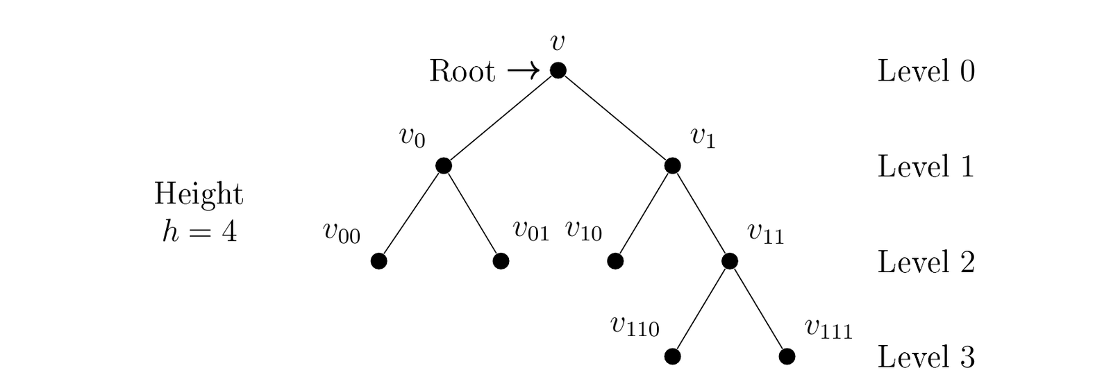
Given two vertices \(X\) and \(Y\) of a binary tree \(T\), we say \(X\) is an ancestor of \(Y\) if \(X\) appears on a level of \(T\) preceding that of \(Y\) and there is a path in \(T\) from \(X\) to \(Y\). (In particular, the root is an ancestor of every other vertex of \(T\).)
Lemma 2.1. The height of a balanced binary tree with \(n \geq 2\) leaves is \(\lceil \log_2 n \rceil + 1\).
Proof. Let \(T\) be a balanced binary tree with \(n \geq 2\) leaves, and let \(\ell \geq 1\) denote the deepest level of \(T\). By the definition of a balanced binary tree, every level from \(0\) to \(\ell – 1\) is full (i.e., every vertex on these levels has two children), while level \(\ell\) contains \(2t\) vertices, arranged in sibling pairs, for some \(t \in \{1, 2, \ldots, 2^{\ell-1}\}\). Among the \(2^{\ell-1}\) vertices on level \(\ell – 1\), exactly \(t\) have children, and the remaining \(2^{\ell-1} – t\) are leaves. Hence the total number of leaves is \[n = \left(2^{\ell-1} – t\right) + 2t = 2^{\ell-1} + t.\]
Since \(1 \leq t \leq 2^{\ell-1}\), this gives \(2^{\ell-1} + 1 \leq n \leq 2^\ell\), and therefore \(\lceil \log_2 n \rceil = \ell\). Because we count levels starting at \(0\), the height of \(T\) (the total number of levels) is \(\ell + 1 = \lceil \log_2 n \rceil + 1\). (For example, in Figure 1 we have \(n = 5\), so \(\ell = \lceil \log_2 5 \rceil = 3\) and the height is \(4\), in agreement with the figure.) \(\square\)
In a balanced binary tree on more than 3 vertices, the root is the unique vertex of degree 2; every other internal vertex has degree 3 (one parent and two children); and every leaf has degree 1.
Lemma 2.2. A balanced binary tree with \(n\) leaves has \(2n – 1\) vertices.
Proof. Let \(q\) be the number of vertices of the tree. Then summing the degrees of those vertices, will give us \(2 (q – 1)\), where \(q – 1\) is the number of edges. We have \(2 (q – 1) = n + 2 + 3 (q – n – 1)\); solving we get \(q = 2n – 1\). \(\square\)
Our main result is Corollary 3.9 and follows from Theorems 3.5 and 3.8.
It is well known (see [4]) that every edge coloring of \(K_n\) in which at least \(n\) colors appear contains a rainbow cycle. On the other hand, rainbow-cycle-forbidding colorings of \(K_n\) using \(n – 1\) colors do exist, and every such coloring forbids monochromatic odd cycles. Hence \(n – 1\) is the largest integer in \(\mathop{\mathrm{MRS}}(K_n;\{\text{odd cycles}\},\{\text{cycles}\})\). We show that every integer between \(\lceil \log_2 n \rceil\) and \(n – 1\) is in \(\mathop{\mathrm{MRS}}(K_n;\{\text{odd cycles}\},\{\text{cycles}\})\). If \(X,Y \subseteq V (K_n)\) are disjoint, then \([X,Y]\) denotes the set of edges in \(K_n\) with one end in \(X\) and one end in \(Y\).
Theorem 3.1 (Gallai’s theorem [3]). Suppose \(n \geq 3\). Let \(k\) be a positive integer. In any \(k\)-edge coloring of \(K_n\) where there is no rainbow \(K_3 \subseteq K_n\), there exists a partition of \(V (K_n)\) into non empty subsets \(V_1, V_2, \ldots, V_t\) (\(t \geq 2\)) such that
(1) for each pair \(i,j\) of integers with \(1 \leq i < j \leq t\), all edges in \([V_i,V_j]\) are colored the same color;
(2) the number of colors on the edges in the set \(\displaystyle\bigcup_{1\leq i<j\leq t} [V_i,V_j]\) is at most \(2\); and
(3) for each \(l \in \{1,\ldots,t\}\), no edge within the complete graph induced by \(V_l\) is colored with any of the \([V_i,V_j]\) colors.
Lemma 3.2. Suppose that \(G\) is a connected graph on \(n > 1\) vertices. Then \(V (G)\) can be partitioned into sets, \(A\) and \(B\), satisfying the following
(1) \(||A| – |B|| \leq 1\), and
(2) \(G [A]\) and \(G [B]\) are connected,
if and only if \(G\) has a spanning tree \(T\) such that for some edge \(e \in E (T)\) such that, if \(T_1\) and \(T_2\) denote the two components of \(T – e\), then \(||V (T_1)| – |V (T_2)|| \leq 1\).
Proof. Suppose \(A\) and \(B\) partition \(V (G)\), with \(||A| – |B|| \leq 1\), and \(G [A]\) and \(G [B]\) are connected. Note that \(n > 1\) implies that \(A \neq \emptyset \neq B\). Let \(T_1\) and \(T_2\) be spanning trees in \(G [A]\) and \(G [B]\) respectively, so \(A = V (T_1)\) and \(B = V (T_2)\). Because \(G\) is connected, there must exist an edge \(e\) with one end in \(A\) and the other in \(B\). Then \(T = T_1 \cup T_2 \cup e\) is a tree satisfying the requirements given in the Lemma.
Conversely, if \(T\) and \(e\) satisfy those requirements, let \(A = V (T_1)\) and \(B = V (T_2)\). Then \(||A| – |B|| \leq 1\), \(G [A]\) and \(G [B]\) have spanning trees \(T_1, T_2\), respectively, and are therefore connected. \(\square\)
Theorem 3.3 ([4]). If \(G\) is a connected graph on \(n\) vertices, then there is a rainbow cycle forbidding edge coloring of \(G\) with \(n – 1\) colors appearing.
Lemma 3.4. Suppose \(n > 1\). An edge coloring of \(K_n\) is rainbow-cycle-forbidding if and only if it is a Gallai coloring.
Proof. The forward implication is clear, since \(K_3\) is a cycle. Now suppose that we have a coloring of the edges of \(K_n\) which is not rainbow-cycle-forbidding. We aim to show that there is a rainbow \(K_3 = C_3\) in \(K_n\), with respect to this coloring.
Let \(m\) be the smallest integer such that there is a rainbow \(C_m\) in \(K_n\). If \(m = 3\), we are done. Otherwise, consider any chord \(uv\) of this \(C_m\). The two edge-disjoint paths along \(C_m\) with ends \(u\) and \(v\), each combined with the chord \(uv\), form two cycles, each of order less than \(m\). The color of \(uv\) can appear on at most one of those two \(uv\) paths, because the \(C_m\) is rainbow; but then there exists a smaller rainbow cycle in \(K_n\), contradicting the choice of \(m\). \(\square\)
Theorem 3.5. For positive integers \(n > 1\) and \(k\), if \(2^{k-1} < n \leq 2^k\) then \([k,\ldots,n – 1] \subseteq\) \(\mathop{\mathrm{MRS}}(K_n;\{\text{odd cycles}\},\{\text{cycles}\})\).
Proof. We will construct a balanced binary tree \(T\) representing a Gallai coloring \(c\). The vertices of \(T\) will be subsets of \(V (K_n) = V\). The root will be the entire vertex set \(V\). For each vertex \(X \subseteq V\) of \(T\), if \(|X| = 1\) then \(X\) is a leaf of \(T\). Otherwise, if \(|X| > 1\), the two “children” of \(X\) at the next “level” of \(T\) will be sets \(Y, Z\) partitioning \(X\), such that \(||Y| – |Z|| \leq 1\). We will refer to \(Y\) and \(Z\) as “siblings.”
The edges of \(K_n\) will be colored as follows: for every pair of sibling vertices \(Y\) and \(Z\) of \(T\), the edges \([Y,Z]\) will be colored with a single color that does not appear on any previously colored edge incident to a vertex in an ancestor of \(Y\) and \(Z\). Such a color always exists: at each step of the construction only finitely many colors have been used so far, so we may always introduce a fresh color (one not previously used) for the pair \((Y,Z)\).
We will enforce this restriction by the requirement that the sets of colors appearing on edges between siblings at different levels be disjoint. Thus, a color may appear on edges between different pairs of siblings, but it may not appear on edges between different pairs of siblings on different levels.
This requirement is stronger than necessary, but it is sufficient for our purposes. We shall see that every such coloring forbids rainbow cycles and monochromatic odd cycles, and the total number of colors appearing can range from \(\lceil \log_2 n \rceil\) to \(n – 1\).
To see this last claim, first note that the binary tree constructed will have \(n\) leaves, one for each vertex of \(K_n\). Therefore, by Lemma 2.2, it will have \(n – 1\) non-leaves, and each of these will have two sibling children, the edges between the sets of vertices corresponding to which will bear one of our colors. Thus we can arrange to have \(n – 1\) colors appear in the coloring by making the colors assigned to the \(n – 1\) sibling pairs distinct.
Now we can reduce the number of colors, one at a time, while honoring the requirement that the sets of colors assigned to the sets of sibling pairs at different levels be disjoint, by merging pairs of colors on the same level. For instance, if, at some stage, blue and burgundy both appear on (edges between sibling pairs on) the same level (and therefore on no other level), we can recolor all burgundy edges blue, thus reducing the total number of colors appearing by one while preserving the disjointness of color sets on different levels.
We can continue counting down in this way until on each level after Level 0 only one color is assigned to sibling pairs on that level. At that point the number of different colors deployed is one less than the number of levels. By Lemma 2.1 the number of levels is \(\lceil \log_2 n \rceil + 1\), so the number of colors is \((\lceil \log_2 n \rceil + 1) – 1 = \lceil \log_2 n \rceil\) (Recall that \(n > 1\).) (Note that this number has not yet been shown to equal min \(\mathop{\mathrm{MRS}}(K_n;\{\text{odd cycles}\},\{\text{cycles}\})\); that will be established in Theorem 3.8.)
Observe that for any color appearing in any colorings obtained above, the subgraph of \(K_n\) induced by the set of edges bearing that color is union of vertex-disjoint complete bipartite graphs. Therefore, there are no monochromatic odd cycles in \(K_n\) with any of these colorings.
It remains to be seen that none of the colorings described allow a rainbow cycle in \(K_n\). Let \(C\) be a cycle in \(K_n\). Let \(X\) be a vertex of \(T\) (therefore, a subset of \(V (K_n)\)) such that \(V (C) \subseteq X\) and, if \(Y\) and \(Z\) are the children of \(X\), then \(V (C) \cap Y \neq \emptyset \neq V (C) \cap Z\). In other words, \(X\) is the vertex of \(T\) on the lowest level of \(T\), among vertices of \(T\) containing \(V (C)\). Since \(C\) is a cycle, \(E (C) \cap [Y,Z]\) must contain at least two edges. Therefore \(C\) is not rainbow. \(\square\)
Theorem 3.6. \(R_2 (K_3) = 6\) [2].
Lemma 3.7. \(\min \mathop{\mathrm{MRS}}(K_4;\{\text{odd cycles}\},\{\text{cycles}\}) = 2\) and \[\min \mathop{\mathrm{MRS}}(K_5;\{\text{odd cycles}\},\{\text{cycles}\}) = 3.\]
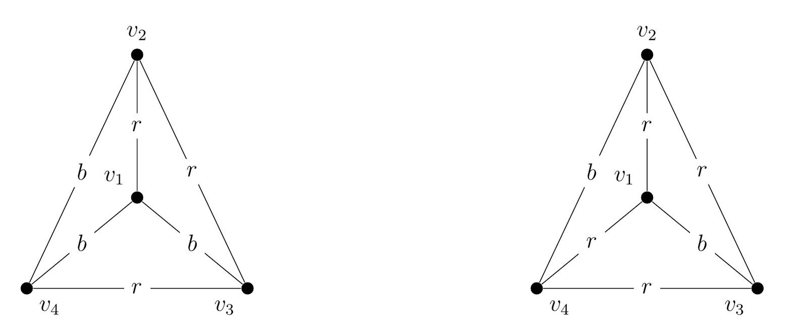
Proof. Clearly \(\min \mathop{\mathrm{MRS}}(K_4;\{\text{odd cycles}\},\{\text{cycles}\}) > 1\), and Figure 2 gives two different edge colorings of \(K_4\) with two colors that admit no monochromatic \(K_3\)’s and no rainbow cycles.
Now suppose that the edges of \(K_5\) are colored with red and blue so that no odd cycle in \(K_5\) is monochromatic. Suppose that \(K_5\) contains a monochromatic \(K_{1,3}\) – suppose edges \(vx,vy,vz\) are colored red. If any of \(xy,xz,yz\) were red then there would be a red \(C_3\) in the edge colored \(K_5\). Therefore all three of those edges are blue, so we have a monochromatic \(C_3\) anyway. So no monochromatic \(K_3\) exists.
It follows that every vertex of \(K_5\) is incident to two red and to two blue edges. The subgraph induced by the blue edges is therefore regular of degree two, so there must be a blue cycle in \(K_5\). It must be a \(C_4\), say on vertices \(v,w,x,y\). Let \(z\) be the vertex of \(K_5\) not in this \(C_4\). Of the four edges incident to \(z\), two are blue, so there must be vertices of \(K_5\) incident to three blue edges, a possibility that has already been ruled out. Thus no such coloring exists.
Since \(3 = \lceil \log_2 5 \rceil\) there is an edge coloring of \(K_5\) with \(3\) colors which forbids monochromatic odd cycles and rainbow cycles by Theorem 3.5. \(\square\)
Theorem 3.8. \(\min \mathop{\mathrm{MRS}}(K_n;\{\text{odd cycles}\},\{\text{cycles}\}) = \lceil \log_2 n \rceil\).
Proof. The proof will be by induction on \(n\). Assume that \(n \geq 6\) and \(K_n\) is edge colored with \(k\) colors appearing so that rainbow cycles and monochromatic odd cycles are forbidden. Since there are no rainbow \(K_3\)’s in \(K_n\), the coloring must be a Gallai coloring as described in Gallai’s Theorem. The number of parts \(t\) in the partition of \(V (K_n)\) in that description must be less than 6 as we know \(R (K_3,K_3) = 6\) from Theorem 3.6. By Lemma 3.7 we know \(t \neq 5\). So \(t \in \{2,3,4\}\).
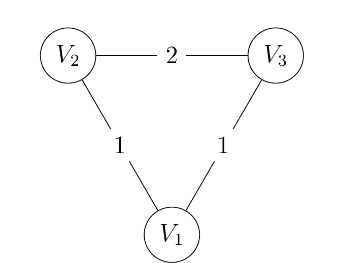
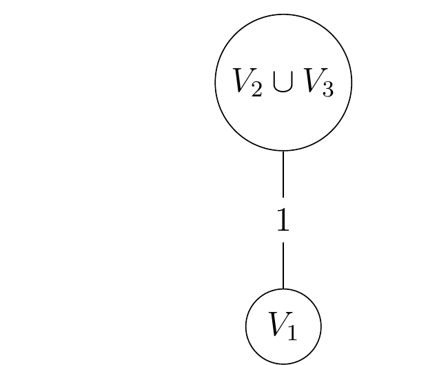
We lifted the following argument from Magnant and Salehi Nowbandegani [5]. Let \(t = 3\). Since we are forbidding monochromatic odd cycles, we must use two colors among the three partitions \(V_1,V_2\), and \(V_3\) as depicted in Figure 3. This puts us in the \(t = 2\) case; see Figure 4.
We are left with cases \(t \in \{2,4\}\). Suppose \(t = 2\) with \(V\) partitioned by \(V_1\) and \(V_2\). Let \(n_1 = |V_1|\), \(n_2 = |V_2|\), and \(n_1 \leq n_2\). Let \(c_1\) and \(c_2\) be the number of colors in \(V_1\) and \(V_2\) respectively with \(c_1 \geq \lceil \log_2 n_1 \rceil\) and \(c_2 \geq \lceil \log_2 n_2 \rceil\). Now \(n_2 \geq \frac{n}{2}\), so we have \[k \geq c_2 + 1 \geq \lceil \log_2 n_2 \rceil + 1 \geq \left\lceil \log_2 \frac{n}{2} \right\rceil + 1 = \lceil \log_2 n \rceil – \lceil \log_2 2 \rceil + 1 = \lceil \log_2 n \rceil.\]
Now suppose \(t = 4\) with a partition by vertex sets \(V_1,V_2,V_3\), and \(V_4\). Let \(n_1 = |V_1|\), \(n_2 = |V_2|\), \(n_3 = |V_3|\), \(n_4 = |V_4|\), and \(n_1 \leq n_2 \leq n_3 \leq n_4\). Let \(c_1, c_2, c_3\), and \(c_4\) be the number of colors in \(V_1,V_2,V_3\), and \(V_4\) respectively with \(c_1 \geq \lceil \log_2 n_1 \rceil\), \(c_2 \geq \lceil \log_2 n_2 \rceil\), \(c_3 \geq \lceil \log_2 n_3 \rceil\), and \(c_4 \geq \lceil \log_2 n_4 \rceil\). Now \(n_4 \geq \frac{n}{4}\), and \[k \geq c_4 + 2 \geq \lceil \log_2 n_4 \rceil + 2 \geq \left\lceil \log_2 \frac{n}{4} \right\rceil + 2 = \lceil \log_2 n \rceil – \lceil \log_2 4 \rceil + 2 = \lceil \log_2 n \rceil.\] \(\square\)
Corollary 3.9. \(\mathop{\mathrm{MRS}}(K_n;\{\text{odd cycles}\},\{\text{cycles}\}) = \{\lceil \log_2 n \rceil,\ldots,n – 1\}\).
Corollary 3.10. If \(k \geq 3\), \(gr_k (\{\text{odd cycles}\} : \{\text{cycles}\}) \leq 2^k + 1\).
Proof. If \(n \geq 2^k + 1\) then \(\lceil \log_2 n \rceil \geq \log_2 n > k\) so, by Corollary 3.9, every \(k\)-edge coloring of \(K_n\) must either contain a rainbow cycle or a monochromatic odd cycle.
By previous arguments (see Lemma 3.7 it can be seen that Corollary 3.10 holds with equality when \(k = 2\). \(\square\)