
Let \(G(V,E)\) be a finite simple graph. Denote by \(|V|\) and \(|E|\) the cardinality of the set \(V\) and \(E\), respectively. Graceful labeling is an injective function \({f}\) from vertex set \({V}\) into the set \(\{0,1,2,…, |E|\}\) which induces a bijective function \(f’\) from edge set \({E}\) onto the set \(\{1,2,…,|E|\}\) such that for every edge \(uv\in E(G)\) we have \({f'(uv)}=|{f(u)- f(v)}|\). A graph that has graceful labeling is called graceful graph. The quantity \(|f(u)-f(v)|\) is frequently called induced label or induced label of the edge \(uv\in G\) or shortly label of the edge \(uv\in G\). Graceful labeling and its variations for classes of graphs are celebrated research topics, see [1, 2, 6, 7, 8, 9, 10, 12, 13]. For more review on this topic we refer to [5].
Let \(G\) be a graceful graph with graceful labeling \(f\). If we find a constant \(\lambda\) for every edge \(uv\in E(G)\) such that \(f(u)\le \lambda<f(v)\), then the function \(f\) is called an \(\alpha\)-\(labeling\), and the graph \(G\) is called an \(\alpha\)-\(graph\). Barrientos and Minion in [4] generalize the concept of \(\alpha\)-labeling as bipartite labeling. A bipartite labeling of \(G\) is an injective function \(f\) from the vertex set \(V(G)\) into the non-negative integer set \(\{0,1,\ldots, s\}\) for which there is an integer \(\lambda\), such that \(f(u)\le \lambda < f(v)\) for every \((u, v)\in A\times B\), that induces \(n\) different labels. Here, \(\{A,B\}\) is a usual bipartition of \(V(G)\), and \(n=|E(G)|\). The integer \(\lambda\) is called the boundary value of \(f\).
All graph classes discussed in this paper do not yet explicitly include classes of chain graphs. In this paper, we will observe some classes of chain graphs with blocks of complete bipartite graphs and derive their \(\alpha-\)labelings. An open chain graph is a graph with blocks \({B_1,B_2,…,B_n}\) such that for every \(i\), \(B_i\) and \(B_{i+1}\) have a common vertex, in such a way that the block-cut-vertex graph is a path. A chain graph having \({n}\) blocks \({B_1,B_2,…,B_n}\) is denoted by \([B_{1},B_{2},…,B_{n}]\). Let \({c_i}\) be the common vertex of \({B_i}\) and \({B_{i+1}}\), in \([{B_1,B_2,…,B_n}]\), \(1\le i \le n-1\). Assume a vertex \(c_0\) in \({B_1}\), \({c_0 \ne c_1}\), and a vertex \(c_n\) in \({B_n}\), \({c_n \ne c_{n-1}}\), \(n\ge 2\), and two vertices \(u\neq v\) in a new connected bipartite block graph \(B\). If we identify the vertex \(c_0\) with \(u\) and the vertex \(c_n\) with \(v\), then the resulting graph is called closed chain graph, and is denoted with \([B_1,B_2,\ldots,B_n,B]_c\). In a closed chain graph, any cut vertex of related open chain graph is no longer cut vertex. Here, we introduce \(\alpha\)-labeling for some chain graphs whose blocks are complete bipartite graphs.
In [3, 11] it is shown that any complete bipartite graphs are \(\alpha\)-graph. We will restate this fact in Theorem 1.2 and give a more detailed proof. Some part of the proof is a tool we refer to in the next discussion.
We start with the following lemma.
Lemma 1.1. Let \(a\) and \(b\) be two integers such that \(b-a=r\ge 1\). Let \(x_1,x_2,\ldots,x_r\) be integers satisfying \(x_{i+1}=x_i+1\) for all \(i=1,2,\ldots,r-1\). Then, the sequence \(x_1-b,x_2-b,\ldots,x_r-b,x_1-a,x_2-a,\ldots,x_r-a\) forms an arithmetic sequence of difference one.
Proof. Since \(x_{i+1}=x_i+1\), it is obvious that for a constant \(c\) we have \(x_{i+1}-c-(x_i-c)=1\). Now we will see that \((x_1-a)-(x_{r}-b)\) is also \(1\) as shown bellow:
\(\square\)
Theorem 1.2 (Barrientos [3], Rosa [11]). The complete bipartite graph
is an \(\alpha\)-graph.
Proof. Let the vertices of \(K_{m,n}\) be \(x_i,y_j:i=1,2,\ldots, m;j=1,2\ldots,n\). Here, the edge set of \(K_{m,n}\) is \(\{x_iy_j:1,2,\ldots,m;j=1,2,\ldots,n\}\). It is clear that the size of \(K_{m,n}\) is \(|E|=mn\). Now, we introduce a labeling \(f:V(K_{m,n})\rightarrow \{0,1,\ldots,mn\}\) as follows:
We can see easily that \(f\) is injective. Moreover, we have that the set \(\{f(x_i):i=1,2,\ldots,n\}=\{0,1,2,\ldots,m-1\}\), and satisfies \(f(x_{i+1})=f(x_{i}+1),\) \(i=1,2,\ldots, m-1\). On the other hand, \(f(y_{j+1})=f(y_j)+m,\) \(j=1,2,\ldots,n-1\). For every \(j=1,2,\ldots,n-1,\) if we take \(a=f(y_j)\) and \(b=f(y_{j+1}),\) then based on Lemma 1.1, we have the sequence
forms an arithmetic sequence of difference one. The smallest edge label is \(|f(y_{1})-f(x_m)|=1\) and the greatest one is \(|f(y_{n})-f(x_1)|=mn\). So, the whole sequence of edge labels is \((1,2,\ldots,mn)\). Therefore, the complete bipartite graph \(K_{m,n},m,n\ge 1\) is graceful. That \(f\) is \(\alpha\)-labeling, we show as follows.
Let the partition sets of \(V\) be \(A=\{x_i:i=1,2,\ldots,m\}\) and \(B=\{y_j:j=1,2,\ldots,n\}\). It is clear, based on Eq. (1), that the greatest label of vertices in \(A\) is \(m-1\) and the smallest label of vertices in \(B\) is \(m\). Therefore, if we take \(\lambda=m-1,\) then we can see that for every \(u\in A\) and \(v\in B\), we have \(f(u)\le \lambda <f(v)\). Thus, \(f\) is an \(\alpha\)-labeling for \(K_{m,n}\), or \(K_{m,n}\) is an \(\alpha\)-graph. \(\square\)
Now, we will observe open chain graphs with blocks of complete bipartite graphs.
Consider the family \(\mathbb{K}(p,r_i)\) of \(n\) complete bipartite graphs \(K_{p,r_i}\), with \(p,r_i\ge 1,\) for every \(1\le i\le n\). Let the vertex set of \(K_{p,r_i}\) be named as the following. For every \(1\le i\le n,\)
and the edge set be
We see that the family \(\mathbb{K}(p,r_i)\) has total size of \(|E|=p\sum\limits^n_{i=1}r_i\). Our open chain graphs will be built from the family \(\mathbb{K}(p,r_i)\), by identifying \(x^i_{r_i}\) with \(x^{i+1}_{1}\), \(1\le i\le n-1.\) If \(r_i=1\) for all \(1\le i\le n\), then this open chain graph is a star graph, and constitutes a caterpillar if \(p=1\). These two graph classes are well known \(\alpha\)-graphs. For a fix positive integer \(p\), for the sake of efficiency, let us denote the resulting open chain graph \([K_{p,r_1},K_{p,r_2},\ldots,K_{p,r_n}]\) as \([\mathcal{K}_{p:r_1,r_2,\ldots,r_n}]\).
The following theorem is formulated in [3].
Theorem 1.3 (Barrientos [3]). Let \(B_1, B_2, \ldots, B_m\) be blocks such that all of them have an \(\alpha\)-labeling. Then, there exists a chain graph \(G\), with blocks \(B_1, B_2, \ldots, B_m\) that accepts an \(\alpha\)-labeling.
From Theorem 1.2 we know that \(K_{p,r}\) is \(\alpha\)-graph, for all \(p,r\geq 1\). Therefore, we have the following consequence of Theorem 1.3.
Corollary 1.4. For \(r_i\ge 1,\) \(1\le i\le n\), the open chain graph \([\mathcal{K}_{p:r_1,r_2,\ldots,r_n}]\) is \(\alpha\)-graph.
Proof. Now, we define a function \(f\) for the family \(\mathbb{K}(p,r_i)\), \(i=1,2\ldots,n\), as follows.
with \(r_0=1\).
Observe that \(f(x^i_{r_i})=f(x^{i+1}_1)\) for all \(1\le i\le n-1.\) This can be seen as the following.
Now we will observe that the above function \(f\) defines a graceful labeling for the open chain graph \([\mathcal{K}_{p:r_1,r_2,\ldots,r_n}]\).
First we see that \(f\) is injective. We can see from Eq. (2) that \(f(c^i_j)=f(c^{i}_{j+1})+1\) for every \(1\le i\le n\) and \(0\le j\le p-1.\) In particular, we have that \(0=f(c^1_0)\le f(c^i_j)\le f(c^n_{p-1})=pn-1\). Whereas from the labels of vertices \(x^i_j\), we also have that \(f(x^i_j)\neq f(x^s_t)\) for every \(i\neq s\) or \(j\neq t\), except \(f(x^i_n)=f(x^{i+1}_0)\). Moreover, we have \(pn=f(x^n_{r_n})\le f(x^i_j)\le f(x^1_0)=|E|\). Thus, \(f\) is injective from \(V([\mathcal{K}_{p:r_1,r_2,\ldots,r_n}])\) into the set \(\{0,1,2,\ldots,|E|\}\). Secondly, we will derive that
Based on Eq. (2), we have for every \(i=1,2,\ldots,n,\)
with \(j=1,2,\ldots,r_i; t=0,1,\ldots,p-1,\) and \(r_0=1\).
Moreover, we can see that \(f\) is \(\alpha\)-labeling. Let the partition sets of \(V([\mathcal{K}_{p:r_1,r_2,\ldots,r_n}])\) be \(A=\{c^i_k:1\le i\le n; 0\le k\le p-1\}\) and \(B=\{x^i_j:1\le i\le n; 1\le j\le r_i\}\). From Eq. (2), we can see the greatest label of \(u\in A\) is \(pn-1\), whereas the smallest label of \(v\in B\) is \(pn\). Thus, if we take \(\lambda=pn-1\), then it is clear that \(f\) is an \(\alpha\)-labeling. \(\square\)
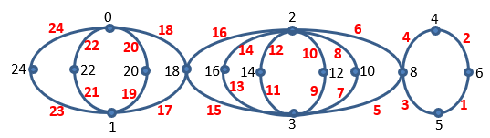
In Figure 1 we show an example of open chain graph \([\mathcal{K}_{2:4,6,2}]\) with its \(\alpha\)-labeling.
Next, we will study closed chain graphs which are built from \([\mathcal{K}_{p:r_1,r_2,\ldots,r_n}]\) and a complete graph \(K_{p,r}\), \(r\ge 2\). Let the vertex set of \(K_{p,r}\), \(r\ge 2\), be
and edge set
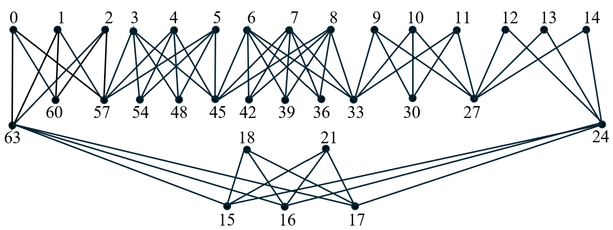
respectively. Then, we identify \(x^1_1\) with \(x_1\) and \(x^n_{r_n}\) with \(x_r\). The resulting graph is a closed chain graph \([\mathcal{K}_{p:r_1,r_2,\ldots,r_n,r}]_c\). In the following part we will show that the closed chain graph \([\mathcal{K}_{p:r_1,r_2,\ldots,r_n,r}]_c\), where \(p,r_i,r,n>1\), is \(\alpha\)-graph. This result is formulated in the following theorem. An \(\alpha\)-graph \([\mathcal{K}_{3:3,4,5,3,2,4}]_c\) is depicted in Figure 2.
Theorem 2.1. For every positive integers \(n,p,r,r_1,r_2,\ldots,r_n\ge 2\), the closed chain graph \([\mathcal{K}_{p:r_1,r_2,\ldots,r_n,r}]_c\) is \(\alpha\)-graph.
Proof. Let \(|E|=p\left(\sum\limits^n_{i=1}r_i+r\right)\), \(\sum\limits^k_{i=1}r_i< n\le\sum\limits^{k+1}_{i=1}r_i\) for some positive integer \(k\), and \(n-\sum\limits^{k}_{i=1}r_i=l\). Define a function \(g\) for \([\mathcal{K}_{p:r_1,r_2,\ldots,r_n,r}]_c\) as follows:
For \([\mathcal{K}_{p:r_1,r_2,\ldots,r_n}]\) part,
with \(r_0=1,\) and for \(K_{p,r}\) part, we set
By some simple algebraic manipulations, it is easy to see that for two vertices \(x^i_{r_i}\) and \(x^{i+1}_{1}\), we have \(g(x^i_{r_i})=g(x^{i+1}_{1})\). Moreover, we also have \(g(x^n_{r_n})=g(x_{r})\), and \(g(x^1_{1})=g(x_1)\).
Here, we will only show that \(g(x^n_{r_n})=g(x_{r})\) as the following.
If we identify all these vertex pairs, namely \(x^i_{r_i}\) and \(x^{i+1}_{r_1}\), \(x^n_{r_n}\) and \(x_{r}\), and the vertex pair \(x^1_{1}\) and \(x_{1}\), then it is easy to observe that for any two vertices \(u,v\) in the mentioned graph we have \(g(u)\neq g(v)\). From here, we may conclude that \(g\) is injective. The greatest and the smallest labels are \(g(c^1_0)=0\) and \(g(x^1_{1})=g(x_r)=|E|\), respectively.
Now we observe the induced edge labels by \(g\).
For every \(i\in \{1,2,\ldots,k,k+2,\ldots,n\}\), we can see that in each \(K_{p,r_i}\), each vertex label \(g(x^i_j)\) with \(j=1,2,\ldots,r_{i},\) will produce \(p\) consecutive induced edge labels \(|g(x^i_j)-g(c^i_s)|:s=0,1,\ldots,p-1\), since \(g(c^i_s)-g(c^i_{s-1})=1:s=1,2,\ldots,p-1\).
Moreover, denote the sets of edge labels \(A,B,C,\) and \(D\) as follows.
We see that for every \(i=1,2,\ldots,n-1\), we have \(g(c^{i+1}_{1})-g(c^{i}_{p})=1\). Therefore, we obtain the following:
Since \(g(c^{k+1}_{l+1})-g(c^{k+1}_{0})=p-1\) and \(g(x^{k+1}_{l})-g(x^{k+1}_{l+1})=2p\), and that \(g(x^i_j)>g(c^t_s)\) for any positive integers \(i,j,s,t\), we get
This informs us that there are exactly \(p\) consecutive positive labels between \(|g(x^{k+1}_{l})-g(c^{k+1}_{p-1})|\) and \(|g(x^{k+1}_{l+1})-g(c^{k+1}_{0})|\). These \(p\) labels are \(|g(x^{k+1}_{l+1})-g(c^{k+1}_{0})|+s\) with \(s=1,2,\ldots,p\). Using Eq.(3) and assumption that \(n-\sum\limits^{k}_{s=1}r_s=l\), we will have that \(|g(x^{k+1}_{l+1})-g(c^{k+1}_{0})|=g(x^{k+1}_{l+1})-g(c^{k+1}_{0})=|E|-p(n+1)\). Therefore, if we denote \(B’=\{|E|-p(n+1)+s:s=1,2,\ldots,p\}\), then the set \(\mathrm{X}= A\cup B\cup B’\cup C\cup D\) in Eq. (6) will constitute the set of consecutive labels started from \(|g(x^{n}_{r_n})-g(c^{n}_{p-1})|=g(x^{n}_{r_n})-g(c^{n}_{p-1})\). Indeed, by using Eq. (4), we can observe that the set formed by the edge labels \(|g(x_1)-g(c_s)|,\) where \(s=0,1,\ldots,p-1\), corresponds to the set \(B’\).
Note that these \(p\) labels are of \(p\) edges \(x_1c_s, s=0,1,\ldots,p-1,\) in the graph \(K_{p,r}\). So, the number of the remaining edge labels in \(K_{p,r}\) which are not observed yet is equal to \(pr-p=p(r-1)\) edges.
On the other side, there are exactly \(p(r-1)\) labels we need to complete edge labels for the whole graph \([\mathcal{K}_{p:r_1,r_2,\ldots,r_n,r}]_c\) to become a graceful labeling. This is shown by using a simple calculation based on Eq. (3) and the fact that \(|E|=p\left(\sum\limits^{n}_{s=1}r_s + r\right)\). Here, we have that the smallest edge label in \(\mathrm{X}\) is \(g(x^{n}_{r_n})-g(c^{n}_{p-1})\) which is equal to \(p(r-1)+1\). This implies that the first \(p(r-1)\) positive integers: \(1,2,\ldots,p(r-1)\), are needed as the edge labels of the remaining edges in order to complete the graceful labeling. Based on Eq. (4), these labels are exactly the labels of the remaining \(p(r-1)\) edges of \(K_{p,r}\), namely edges \(x_{j}c_s\) where \(j=2,3,\ldots,r;s=0,1,\ldots,p-1\). These labels are
with \(j=2,3,\ldots,r;s=0,1,\ldots,p-1.\) Until here, we have proven that \(g\) is a graceful labeling for \(\mathcal{K}_{p:r_1,\ldots,r_n,r}\). Next, we will show that \(g\) is an \(\alpha\)-labeling. This is clearly seen from Eq. (3) and Eq. (4), that
with \(i=1,2,\ldots,n;s=0,1,\ldots,p-1;j=1,2,\ldots,r_i;t=1,2,\ldots,r.\) So, by taking \(\lambda = g(c_{p-1}),\) then we can conclude that \(g\) is an \(\alpha\)-labeling, and therefore the graph \([\mathcal{K}_{p:r_1,r_2,\ldots,r_n,r}]_c\) is an \(\alpha\)-graph. \(\square\)
Now, we will study another type of chain graph, but with a particular block graphs. Here, we will focus on chain graphs with complete bipartite graph \(K_{p,r}\), \(r\ge 1\), with \(p=2\).
Remark 2.2. In case \(r\) is even, instead of using the labeling in Eq. (1), we may also apply the following function to prove Theorem 1.2:
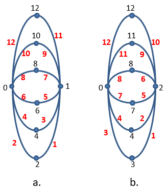
See Figure 3 for the comparison.
To proceed to the main observation here, we introduce the following lemma which constitutes a tool in the next discussion.
Lemma 2.3. Let \(f\) be the graceful labeling of the graph \(K_{2,r}\), with vertices \(c_1,c_2, x_i: i=1,2,\ldots,r\). If \(r\) is odd, then the parity of \(f(c_1)\) and \(f(c_2)\) can not be the same.
Proof. Let \(f\) be any graceful labeling for \(K_{2,r}\). Here, stable sets of \(V(K_{2,r})\) are \(\{c_1, c_2\}\) and \(B=V(K_{2,r})\backslash \{c_1, c_2\}\). It is clear that for every vertex \(x\) in \(V(K_{r,2})\backslash \{c_1,c_2\}\), we have that the parity of \(|f(x)-f(c_1)|\) and \(|f(x)-f(c_2)|\) are the same, whenever \(f(c_1)\) and \(f(c_2)\) have the same parity. Since \(r\) is odd, we obtain that the difference between the number of odd edge labels and of even edge labels is a positive even integer. This implies that those all induced edge labels can not form an arithmetic sequence with difference one. This violates the function \(f\) as a graceful labeling. \(\square\)
Assume that we have a family of \(n\) graphs \(K_{2,r_j}\), \(1\le j\le n\), with \(r_j\ge 1\). For every \(k=1,2,\ldots,n,\) let the vertex set and edge set of \(K_{2,r_k}\) be \(\{c^k_1,c^k_2,x^k_j:j=1,2,\ldots, n,\}\) and \(\{c^k_1x^k_j,c^k_2x^k_j:1\le j\le n\}\). Partition the vertex \(V(K_{2,r_k})\) into the stable sets \(A_k=\{c^k_1,c^k_2\}\) and \(B_k=\{x^k_j:j=1,2,\ldots,n\}\).
The second type of chain graph here is constructed by identifying \(c^{j}_2\) and \(c^{j+1}_1,\) for all \(j,1\le j\le n-1\). For the sake of efficiency, the resulting open chain graph \([K_{2,r_1},K_{2,r_2},\ldots,K_{2,r_n}]\) will be denoted as \([\mathcal{K’}_{2:r_1,r_2,\ldots,r_n}]\). Here, the size of this chain graph is \(|E’|=\sum\limits^n_{i=1}|E_{i}|=2\sum\limits^n_{i=1}r_i\). Note that if \(r_i=1\) for every \(1\le i\le n\), then the open chain graph \([K_{2,r_1},K_{2,r_2},\ldots,K_{2,r_n}]\) forms a path graph. Again, it is well known that any path is \(\alpha\)-graph.
Here, again we have a corollary of Theorem 1.3.
Corollary 2.4. For every positive integers \(r_i:i=1,2,\ldots,n,\) the open chain graph \([\mathcal{K’}_{2:r_1,r_2,\ldots,r_n}]\) is \(\alpha\)-graph.
We will propose a proof for the Corollary to facilitate the proof of Theorem 2.5.
Proof. It is clear from Theorem 1.2 that \(K_{2,r_i},i=1,2,\ldots,n,\) is \(\alpha\)-graph. Assume the \(\alpha\)-labeling for \(K_{2,r_i}\) is \(f_i\) as defined in Eq. (1) for \(m=2\) and \(n=r_i\).
For every \(k,1\le k\le n,\) we have that the smallest (resp. biggest) label in \(K_{2,r_k}\) is \(|f_k(x^k_{1})-f(c^k_{2})|=1\)(resp. \(|f_k(x_{n})-f_k(c^k_1)|=|2r_k-0|=|E_k|\)). First we will proceed to see that \([\mathcal{K’}_{2,r_{n-1},r_{n}}]\) is graceful by using the following procedure.
Define a function \(g_1\) for \([\mathcal{K’}_{2,r_{n-1},r_n}]\) as follows:
Since all vertex labels of \(K_{2,r_n}\) is added up with the same constant \(1\), the set of edge labels of the re-labeled \(K_{2,r_n}\) by \(g_1\) remains the same, that is equal to \(\{1,2,\ldots,|E_{r_n}|\}\).
Now let us see the new edge labels of \(K_{2,r_{n-1}}\) by \(g_1\). Since all old labels except the labels of \(c^{n-1}_i, i=1,2,\) each is augmented by \(|E_{r_n}|\), we get that the set of new edge labels of \(K_{2,r_{n-1}}\) is \(\{1+|E_{r_n}|,2+|E_{r_n}|,\ldots,|E_{r_{n-1}}|+|E_{r_n}|\}.\) Now we identify \(g_1(c^{n-1}_2)=1\) and \(g_1(c^{n}_1)=1\). It is easy to observe that the resulting open chain graph \([\mathcal{K’}_{2,r_{n-1},r_n}]\) is graceful with the biggest edge label \(|E_{r_{n-1}}|+|E_{r_n}|\). Moreover, if we take \(\lambda=2\), then we may conclude that this open chain graph is \(\alpha\)-graph.
Now we will see a similar procedure for labeling open chain graph \([\mathcal{K’}_{2,r_{n-j},r_{n-{(j-1)}},\ldots,r_{n}}]\), \(1\le j\le n-1\). We proceed using the following function \(g_j\) for \(2\le j\le n-1\).
After identifying \(c^{n-j}_2\) and \(c^{n-(j-1)}_1\) with \(g_j(c^{n-j}_2)=1=g_j(c^{n-(j-1)}_1)\), and using the same argument as in case \([\mathcal{K}_{2:r_{n-1},r_{n}}]\), we can conclude that the chain graph \([\mathcal{K’}_{2:r_{n-{(j-1)}},r_{n-{(j-2)}},\ldots, r_n}]\) is graceful. Here, we can conclude that this open chain graphs is \(\alpha\)-graph by taking the boundary constant \(\lambda=j\).
Continuing this process \(n-1\) times, we finally may conclude that \([\mathcal{K’}_{2:r_{1},r_{2},\ldots, r_n}]\) is \(\alpha\)-graph with \(\lambda=n\). \(\square\)
Consider an open chain graph \([\mathcal{K’}_{2:r_1,r_2,\ldots,r_n}]\). Recall that the vertex \(c^j_2\) of the graph \({K}_{2,r_j}\) is identified with the vertex \(c^{j+1}_1\) of the graph \({K}_{2,r_{j+1}}\), for all \(1\le j\le n-1\). We will name these identified vertices \(c^j_{2}=c^{j+1}_1\) shortly as \(c_{j}\), for all \(1\le j\le n-1\), \(c^{1}_1\) as \(c_0\), and \(c^{n}_2\) as \(c_n\). Thus, in the open chain graph \([\mathcal{K’}_{2:r_1,r_2,\ldots,r_n}]\), we have vertex set
and edge set
For \(n\ge 2,\) if \(c_n\) and \(c_0\) are identified, the resulting chain graph is closed, and is denoted by \([\mathcal{K’}_{2:r_1,r_2,\ldots,r_n}]_c\).
In the following, we will show that the closed chain graph \([\mathcal{K’}_{2:r_1,r_2,\ldots,r_n,r}]_c\) is \(\alpha\)-graph for some pairs of positive integers \(r\) and \(n\). This result is formulated in Theorem 2.5.
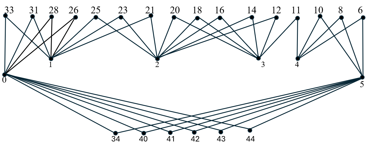
In Figure 4 we show an example of the closed graph \([\mathcal{K’}_{2:4,3,5,1,3,6}]_c\) with its \(\alpha\)-labeling. In this example the values of \(n, r,\) and \(r’\) are \(5, 6\), and \(1\), respectively.
In the sequel, for every \(i=1,2\ldots,n\) we partition every vertex set \(V(K_{2,r_i})\) into stable sets \(A_i=\{c_{i-1},c_{i}\}\) and \(B_i=\{x^i_j:j=1,2,\ldots,n\}\).
Theorem 2.5. Let \(n\) and \(r\) be positive integers, and \(r\equiv r'(\text{mod }n)\). If \(n\) and \(r’\) have the same parity, and \(r_1,r_2,\ldots,r_n\) are any positive integers, then the closed chain graph \([\mathcal{K’}_{2:r_1,r_2,\ldots,r_n,r}]_c\) is \(\alpha\)-graph.
Proof. Based on Corollary 2.4, the chain graph \([\mathcal{K’}_{2:r_1,r_2,\ldots,r_n}]\) is \(\alpha\)-graph. Let \(f\) be the \(\alpha\)-labeling for the open chain graph \([\mathcal{K’}_{2:r_1,r_2,\ldots,r_n}]\) as described in the proof of Corollary 2.4. Here, \(f(c_j)=j\), \(j=0,1,\ldots,n\). The greatest vertex label of \([\mathcal{K’}_{2:r_1,r_2,\ldots,r_n}]\) is \(|E|=2\sum\limits^n_{i=1}r_i.\) which is equal to the size of \([\mathcal{K’}_{2:r_1,r_2,\ldots,r_n}]\).
Note that in the \(\alpha\)-graph \([\mathcal{K’}_{2:r_1,r_2,\ldots,r_n}]\), we have that for every \(j=1,2,\ldots,n,\)
Now consider the complete bipartite graph \({K}_{2,r}\) with stable sets \(A=\{v_0,v_1\}\) and \(B\) which will be set based on two cases: \(r\le n\) and \(r>n\). If \(r\le n\), then \(B=\{y_1,y_2,\ldots,y_r\}\), and if \(r>n\), let us say \(r=kn+r’\) for some integers \(k\ge 0\) and \(1\le r'<n\), then \(B=\{y^{j}_{i}:1\le j\le k,1\le i\le n\}\cup \{y^{k+1}_{i}:1\le i\le r'\}\).
Introduce first a vertex labeling \(g\) for \({K}_{2,r}\) as follows.
Case \(r\le n\). Here \(r=r’\).
We see that \(g(y_{i-1})-g(y_{i})=1\), \(1\leq i\leq r\). These vertex labels will produce \(2\) sequences of edge labels(each sequence is arranged increasingly):
and
The difference between the smallest of the first sequence and the largest of the second sequence is \(|E|+r+1-(|E|+2r-n)=n-r+1\). This means that we need \(n-r\) edge labels to be inserted such that from those above two sequences of edge labels we have an arithmetic sequence of difference one. Note that \(n-r\) is even, since \(n\) and \(r\) have the same parity. Let \(B_0\) be the empty set and \(r_0=0.\) If \(\sum\limits^{j}_{i=0}r_{i}< (n-r)/2\le \sum\limits^{j+1}_{i=0}r_{i}\) for some \(0\le j\le n-1\), then these \(n-r\) edge labels will be produced by relabeling \((n-r)/2\) vertex labels of \(\cup^j_{i=0}B_i\) and of the \(s\) vertex labels of \(B_{j+1}\), with \(s=\frac{n-r}{2}-\sum\limits^j_{i=0}r_i\). These new relabeled vertices will produce all edge labels needed to complete the mentioned gap of edge labels.
For the above value of \(0\le j\le n-1,\) let the set of all vertices in \(\cup^j_{i=0}B_i\) and in the set of the first \(s\) vertices of \(B_{j+1}\) be denoted as \(R\). We will extend the function \(g\) for every \(v\in R\) using the following rule.
Now observe the vertex labels of \(x^1_1\) and \(x^{j+1}_{s}\). We will show that \(g(x^{1}_{1})=g(y_r)-1\) and \(g(x^{j+1}_{s})-(j+1)=g(y_1)-n+1\). If these are proved, the resulting sequence will complete the mentioned gap.
We have
and
Let the vertex \(u\) be the successor of the vertex \(x^{j+1}_{s}\) which is possibly in \({K}_{2,r_{j+1}}\) or in \({K}_{2,r_{j+2}}\) such that it is either \(f(u)-j=f(x^{j+1}_{s})-(j+1) – 1\) if \(u\in {B}_{j+1}\), or \(f(u)-{j+1}=f(x^{j+1}_{s})-(j+1) – 1\) if \(u\in {B}_{j+2}\). In this last case, the vertex \(u\) is actually the vertex \(x^{j+2}_1\). Now we will show that
or
First, assume that \(u\in {B}_{j+1}\). Thus,
Secondly, assume that \(u\in {B}_{j+1}\). Here we have,
Now, we extent the function \(g\) to all \(w\in V([\mathcal{K’}_{2:r_{1},r_{2},\ldots,r_{n}}])\backslash R\), such that \(g(w)=f(w)\). Then, to produce the closed chain graph \([\mathcal{K’}_{2:r_{1},r_{2},\ldots,r_{n},r}]_c\) using the open chain graph \([\mathcal{K’}_{2:r_{1},r_{2},\ldots,r_{n}}]\) and the complete bipartite graph \(K_{2,r}\), we identify vertices \(v_0\) with \(c_0\) and \(v_1\) with \(c_n\). Note that \(g(v_0)=g(c_0)=0\) and \(g(v_1)=g(c_n)=n\). Then, we can immediately see that the extended function \(g\) is a graceful labeling for the closed chain graph \([\mathcal{K’}_{2:r_{1},r_{2},\ldots,r_{n},r}]_c\).
Moreover, we see that the stable set \(\{c_0,c_1,\ldots,c_n\}\) of \(V([\mathcal{K’}_{2:r_{1},r_{2},\ldots,r_{n},r}]_c)\) has labels set \(\{g(c_i):i=0,1,\ldots,n\}=\{0,1,\ldots,n\}\), and all vertex labels of the other stable set are greater than \(n\). Thus, by taking \(\lambda=n\) we can conclude that the function \(g\) is an \(\alpha\)-labeling, and therefore the resulting closed chain graph is \(\alpha\)-graph.
Case \(r>n\), say \(r=kn+r’\), \(0\le k,1\le r'< n\). Here we set a vertex labeling \(g\) for \(K_{2,r}\) as the following
Note that for each \(j\), any \(n\) vertex labels \(\{g(y^j_i):i=1,2,\ldots,n\},\) will form an arithmetic edge labels \(\{g(y^j_1),g(y^j_2),\ldots,g(y^j_n),g(y^j_1)-n,g(y^j_2)-n,\ldots,g(y^j_n)-n\}\), with difference one.
We can see from Eq. (12), that for every \(1\le j\le k,\) we have \(g(y^j_n)-n-g(y^{j+1}_1)=1.\) This implies that the set of edge labels \(\{g(y^j_i),g(y^j_i)-n:j=1,2,\ldots,k;i=1,2,\ldots,n\}\) is equal to the set \(\{g(y^k_n)-n,g(y^k_n)-n+1,\ldots,g(y^1_1)=|E|+2r\}\). Therefore, if we think \(r’\) as \(r\) in the case \(r\le n\), then the case becomes the same with the case \(r\le n\). Thus, again we can conclude here that the closed chain graph \([\mathcal{K’}_{2:r_{1},r_{2},\ldots,r_{n},r}]_c\) is \(\alpha\)-graph.
In any case, we have shown that the closed chain graph \([\mathcal{K’}_{2:r_{1},r_{2},\ldots,r_{n},r}]_c\), is \(\alpha\)-graph for \(r-n\) even. \(\square\)
Observe that the closed chain graph \([\mathcal{K’}_{2:r_{1},r_{2},\ldots,r_{n},r}]_c\) is equivalent to the closed graph \([\mathcal{K’}_{2:r_{i+1},\ldots,r_n,r, r_1,\ldots, r_{i-1},r_i}]_c\). Furthermore, we also see from the proof of Theorem 2.5 that there is no restriction on the values of \(r_i: 1\leq i \leq n\). Therefore, if in case \(n\) and \(r’\) are not with the same parity, but there exists \(r_i\), for some \(1\leq i\leq n\), such that \(n\) and \(r_i’\) have the same parity, with \(r_i\equiv r_i’\pmod n\), then the graph \([\mathcal{K’}_{2:r_{1},r_{2},\ldots,r_{n},r}]_c\) is also \(\alpha\)-graph. In here, the role of \(r\) is replaced by \(r_i\). This observation is formulated as the following corollary.
Corollary 2.6. The graph \([\mathcal{K’}_{2:r_{1},r_{2},\ldots,r_{n},r}]_c\) is an \(\alpha\)-graph if there exists \(r_i\) for some \(1\leq i\leq n\), such that \(n\) and \(r_i’\) have the same parity, with \(r_i\equiv r_i’\pmod n\).
We construct some chain graphs and the closed one with blocks of complete bipartite graphs. Here, a stable set of all complete bipartite graph has the same order. The first chain graphs we observe here are built by identifying vertices of these bipartite graphs which are belong to the other partition. We may call this as chain graph of type I. We can also construct chain graph of type II by identifying vertices from the partitions having the same order. Here, we introduce a labeling for type I chain graphs and proved that the labeling is an \(\alpha\)-labeling. So, these type I chain graphs are \(\alpha\)-graphs. Whereas, observation for type II chain graphs is still limited to a specific complete bipartite graphs with a stable set of cardinality two. Observation of more general chain graphs of type II is an ongoing work.
We closed our paper with the following open problem.
Let \(B_i\) be any complete bipartite graph for every \(i=1,2,\ldots,n\) and \(c^i_1\neq c^i_2\) be any two different vertices in \(B_i\). Identify \(c^i_2\) with \(c^{i+1}_1\) with \(i=1,2,\ldots,n-1\). The resulting chain graph is named as type III chain graph. Now, we have the following open research problem.
Problem 3.1. Do the chain graphs of type III constitute \(\alpha\)-graphs?