
Underground pipe culverts are a vital component of urban infrastructure and are essential to the design and maintenance of urban areas [1, 2]. Nonetheless, finding and locating subterranean pipe culverts has proven to be a significant challenge in urban planning and engineering development because of their lengthy construction times and lack of knowledge. The conventional manual inspection approach is constrained by time and space, and the emerging technology encounters numerous challenges when attempting to detect the contents of pipe culverts, including their lengthy length, water-filled interiors, and exteriors covered in concrete, soil, and water [3, 4].
When it comes to finding and identifying subterranean pipe culverts, researchers in the technical and academic domains have been actively investigating a number of approaches. The combined use of inertial location, video surveillance, and remote-controlled robots has gained a lot of interest as a solution in recent years. In addition to offering new opportunities for the development of smart cities, this integrated technology can precisely identify the internal state and geographical location of subterranean pipe culverts, which is crucial for supporting urban drainage and sewage pulse [5, 6]. A few other elements that significantly add to the subterranean pipe culvert’s complexity and diversity include its depth, laying method, and cross position. The conventional pipeline placement and detection techniques have not been able to keep up with the demands of this complicated environment, and new technical methods are desperately needed to increase the efficiency and accuracy of detection.
With the advancement of technologies such as laser scanning, global positioning systems (GPS), geographic information systems (GIS), and others, a number of innovative techniques and instruments have been developed in the field of underground pipe culvert identification in recent years [7]. Among them, the subterranean pipe culvert’s three-dimensional reconstruction technology based on laser scanning and radar measurement can accomplish precise positioning and high-precision detection. Urban infrastructure management can be greatly aided by the accurate location and three-dimensional visualisation of subterranean pipe culvert networks, which can be accomplished by integrating laser scanning data with GIS [8].
Nevertheless, there are drawbacks to laser scanning technology as well, namely the need for costly hardware and intricate data processing, which restricts its use and promotion in real-world settings [9]. Consequently, one of the research hotspots for the demands of underground pipe culvert detection is the pipe collision detection method based on the projection in the direction of the common perpendicular. By computing the relative position relations between pipes, the approach effectively identifies and localises the collision scenario of an underground pipe culvert by utilising the geometric features and projection relations of the pipe. The method may precisely determine the collision scenario between pipelines by taking into account the expected position of the underground pipe culvert in a vertical direction. This provides crucial technical support for the management and development of urban infrastructure.
One of the most important factors in subterranean pipe culvert identification, in addition to the pipe collision detection technique, is the minimum distance calculation technique from the point to the ellipse. To maintain the stability and safety of pipeline operation, it is frequently required to locate and monitor the surrounding environment in the subterranean pipe culvert network [10]. By carefully examining the ellipse’s shape and the point’s location, the minimal distance calculation method from the point to the ellipse enables efficient environmental monitoring and positioning around the subterranean pipe culvert. The minimal distance between the point and the ellipse can be precisely determined by computing the geometric relationship between the elliptical form and the point, offering a crucial technological tool for the location and identification of subterranean pipe culverts.
The current techniques for detecting collisions and subterranean pipe culverts still have certain drawbacks and difficulties, albeit [11]. For instance, the algorithms’ efficiency and accuracy still need to be increased, and they are not yet perfect in handling scenarios including numerous pipeline crossings and complicated terrain. Furthermore, the practical application of underground pipe culvert detection and positioning technology also faces issues related to data sharing and privacy protection. These issues must be thoroughly examined from the perspectives of technology, law, economy, and other relevant factors in order to foster technological innovation and the advancement of applications [12].
In order to increase the detection precision and positioning accuracy of subterranean pipe culverts, this study intends to investigate the pipeline collision detection method based on the projection of the direction of the common perpendicular and the minimum distance calculation technique from the point to the ellipse. This work attempts to provide helpful reference and guidance for future research in the field of underground pipe culvert identification and collision detection through theoretical analysis and experimental verification. Concurrently, this research will investigate the trajectory of advancement and potential uses of subterranean pipe culvert detection technologies, offering fresh concepts and approaches for managing and building urban infrastructure.
The cylinder is first reduced to a central axis (centre line) for analytical purposes. Two cases coplanar and anisotropic define the spatial relationship between two lines, \({g_1}\) and \({g_2}\), in three dimensions.
When the two are coplanar, their spatial relationship can be classified as intersecting, parallel, co-linear, intersecting extension lines, parallel extension lines, co-linear extension lines, and so forth. Figure 1(left) through 1(right) illustrates these relationships. The projected length of the two segments won’t be shortened, it should be noted, because the plane that houses \({g_1}\) and \({g_2}\) is a space plane that was jointly chosen by the two rather than a horizontal projection plane.
The spatial relationship between \({g_1}\) and \({g_2}\) on the projection plane is only intersected by two cases when anisotropic projection is chosen-intersecting and intersecting the extension line. This is due to the choice to project along the common perpendiculars of \({g_1}\) and \({g_2}\).
Given that the perpendicular distance between the central axes is \(d\) and the radii of the two cylinders are \({r_1}\) and \({r_2}\), respectively, the two cylinders collide as follows, accounting for the cylinders’ respective radii:
Since \(d\) is 0,\({r_1}>0 and {r_2}>0\), the cylinders will collide when the medial axes are coplanar and intersect or co-linear.
When the extension lines are parallel or coplanar and the centre axis is coplanar, there is no collision for all values of \(d\), \({r_1}\) and \({r_2}\).
If \(d=<{r_1}+{r_2}\), the cylinders collide if the centre axes are coplanar and parallel.
Let \({L_{\min }}\)be the shortest distance between the two central axis segments and be the angle between the line segments where the extension lines intersect the coplanar central axis. The precise requirement for the two lines to collide is \({L_{\min }}{r_1} + {r_2}\cos \theta\) if the shortest distance is the scenario depicted in Figure 1(left) and \({L_{\min }}\) is equal to the length of the vertical line AB; The specific circumstances for the two pipes to collide are \({L_{\min }}\sqrt {B{F^2} + D{F^2}}\), where \(DF = {r_1}\sin \theta ,BF = {r_1}\cos \theta + {r_2}\), if the shortest distance is represented by the scenario in Figure 1(right) and \({L_{\min }}\) is equal to the length of the line BD connecting the two closest endpoints.
Apart from the two scenarios illustrated in Figure 1, there exist more scenarios in which the co-axial segments and their extensions cross. These scenarios result in disparate approaches to computing \({L_{\min }}\) and incoherent collision assessment criteria. The collision condition in literature [13, 14] is \({L_{\min }}{r_1} + {r_2}\), which only offers an approximative technique of judging. The projection of two cylinders in the common plane can be thought of as two rectangles, \({r_1}\) and \({r_2}\), and if \({r_1}\) and \({r_2}\) intersect, it indicates that the cylinders are intersecting, which changes the collision of the cylinders into the intersection of two rectangles in any direction. This allows one to accurately calculate whether a collision occurs or not [13].
The axis separation method can be used to ascertain whether or not the two rectangles ABCD and PQTS meet[14], as depicted in Figure 2(left). The coordinates of each of the two rectangles’ four vertices are known. The X’ and Y’ axes are used as the projection axes to judge the overlap of the two rectangles in the projection axis; similarly, rotate the coordinate system so that the X-axis is parallel to another rectangle’s any side, and make the same judgement. This is demonstrated in Figure 2(right). Initially, rotate the coordinate system so that the X-axis is parallel to any side (assumed to be AD) of any rectangle (assumed to be ABCD). As a result of projection along the four projection axes, it is determined that there is no collision between the two rectangles if there is no overlap between them in one direction of the projection axis (referred to as the separate projection axis); if not, it is determined that there is a collision. The two rectangles clearly do not overlap in the Y’ axis, as seen in Figure 2(right), indicating that they do not collide.
There won’t be a collision if the common perpendicular’s length \(L\) is more than the total of the two radii; if not, the positional relationship between the two axis segments must be examined, which can be broadly classified into the next two scenarios:
The two perpendiculars of the common perpendicular, or the intersection of the centre axes’ projections, are in the centre axis segment if the centre axes are opposite to one another and the projections intersect in the common perpendicular’s direction. The two cylinders’ collision condition is \(L \le{r_1}+{r_2}\), if the length of the common perpendicular is \(L\).
At least one of the two pendant feet of the common perpendicular does not reside in the line segment of the axis when the axes are opposed to one another and the projected extensions intersect in the common perpendicular’s direction. To analyse the spatial relationship between the two cylindrical projections, the axes are first split into two cases based on their angle: vertical and inclined. In each case, potential cases of changing the distance in the vertical direction are examined, and in the case where the vertical directions intersect, potential cases of changing the distance in the horizontal direction are also considered (see Figure 3).
When two cylinders collide, it is evident that at least one of the cylinders’ end faces must be involved in the collision and the projected extensions must intersect. If not, the centre axes projected along the perpendiculars must intersect even if no end face is involved in the collision. In this instance, the cylinders’ intersection can be reinterpreted as a determination of whether all of the two cylinders’ end faces intersect with a different cylinder that does not contain the end face. Subsequently, the cylinders can be intercepted using the plane of their end faces, producing rectangles with two cross-sectional forms and ellipsoids (occasionally a partial ellipse due to the cylinders’ limited length) [15]. Different cross-sections are the result of the cylinders \({g_1}\) and \({g_2}\)’s differing sizes and locations. The cutting plane positions are indicated by the red dotted lines in Figure 3, which depicts five representative cases. Cutting \({g_1}\) with one face of \({g_2}\) produces a rectangular cut when the centre axes of \({g_1}\) and \({g_2}\) are perpendicular; cutting \({g_1}\) with one face of \({g_2}\) produces an elliptical (or partially elliptical) cross-section when the centre axes of \({g_1}\) and \({g_2}\) are inclined.
As can be seen from Figure 4, the problem of determining the intersection of two cylinders is actually converted to the problem of the minimum distance between a circle and an ellipse or a circle and a line segment in a restricted domain. Assuming that the minimum distance from a circle to a segment or from a circle to an ellipse is \(|PQ|\), the minimum distance from the centre of a circle to a segment or from the centre of a circle to an ellipse is \(|OP|\), and the radius of the end face of a circle is , then there exists a problem of \(|PQ|= |OP|- r_2\) when the two circles are separated, and the minimum distance from a circle to a segment becomes a problem of the minimum distance from a point (circle centre \(O\)) to a segment, and the minimum distance from a circle to an ellipse becomes a problem of the minimum distance from a point to an ellipse. The minimum distance from the circle to the ellipse becomes the minimum distance from the point to the ellipse. At this point, the condition for determining the collision of \({g_1}\) and \({g_2}\) becomes \(|OP|\le r_2\) [16, 17].

The relative positions and diameters of the cylinders \({g_1}\) and \({g_2}\) are related to their collision, but the coordinate reference system is not. It is necessary to build a new coordinate system in order to perform calculations. Let us assume that \({g_1}\) has radius \({r_1}\), \({g_2}\) has radius \({r_2}\), and \(\theta\) is the angle between \({g_1}\) and \({g_2}\). The relationship depicted in Figure 5 is obtained by truncating the cylinder \({g_1}\) with the cylindrical end of \({g_2}\), generating a circle \({c_3}\), and the cross section of \({g_1}\) forming an ellipse. It is evident that the radius of circle \({c_3}\) is \({r_2}\), the long semiaxis of the ellipse is \(r_1/\cos\theta\), and the short semiaxis is \({r_1}\) [18].

A customised two-dimensional coordinate system for the plane in which the ellipse and the circle lie together (the section) is called the section coordinate system. The coordinate system takes the geometric centre \(O\) of the ellipse as the origin, the long axis as the x-axis, and the short axis as the y-axis, as shown in Figure 5(b). In the new coordinate system, the longitudinal coordinate of \({c_3}\) is the length of the common perpendicular of the two columns, and its transverse coordinate is \(|c_{3}f|/\cos\theta\); the corresponding transverse coordinates of the b-points are \(|c_{3}f|/cos\theta-r_2\), and the corresponding transverse coordinates of the e-points are \(|c_{3}f|/\cos\theta+r_2\). At this point, the standard equations of the ellipse can be easily determined and the coordinates of the centre of the circle, \(|c_{3}\), can be determined. \({g_1}\) and \({g_2}\) collision problem becomes a collision if the minimum distance from a moving point p on the ellipse to the fixed point \(c_{3}\) is less than \(r_{2}\). The equation of the ellipse is as follows:
\[{{{x^2}} \over {{{\left( {{r_1}/\cos \theta } \right)}^2}}} + {{{y^2}} \over {{r_1}^2}} = 1.\tag{1}\]
When the cylinder is sliced with a cross-section, the resulting cross-section might not be a full ellipse because of the influence of the circle and ellipse’s size and relative positions. With the exception of two situations, 1 and 4, as illustrated in Figure 6(a), the cross-section results in a partial ellipse when \({g_1}\) is cut at positions 2, 3, 5, 6, and 7. In this instance, one must compute the distance between a point p on the ellipse and the fixed point \(c_{3}\) such that p lies inside a defined domain, or the partial ellipse’s x-axis projection.
In the cross-sectional coordinate system, in order to judge the boundaries of some ellipsoids, we can first judge whether the intersection point o is in the interior or exterior of \({g_1}\), and then judge the lengths of the projections of \(c_{1}\) and \(c_{2}\) on the projection line ag of the cutting plane (i.e., \(|oc|, |og|\)). Take Figure 6(b) as an example, the specific calculation process is as follows: first calculate the lengths of \(|oc_{1}|, |oc_{2}|, |c_{1}c_{2}|\), and then calculate the lengths of the projections of \(oc_{1}\) and \(oc_{2}\), on the projected line ag as \(|oc| and |og|\). The length of \(|od|\)(ellipse long half-axis) is \(r_{1}/\cos\theta\) [19].
Given an ellipse with equation \({{{x^2}} \over {{a^2}}} + {{{y^2}} \over {{b^2}} = 1}\), a moving point on it \(M({x_m},{y_m})\), and a point \((P (m, n))\) outside of it, the square of the distance between the point and the ellipse is:
\[f\left( {{x_m},{y_m}} \right) = |PM{|^2} = {\left( {m – {x_m}} \right)^2} + {\left( {n – {y_m}} \right)^2} = {m^2} + {n^2} – 2m{x_m} – 2n{y_m} + {x_m}^2 + {y_m}^2,\tag{2}\] and since \(M({x_m},{y_m})\) satisfies the elliptic equation \({{{x_m}^2} \over {{a^2}}} + {{{y_m}^2} \over {{b^2}}} = 1\), we have: \[{y_m} = \pm \sqrt {{b^2} – {{{b^2}} \over {{a^2}}}{x_m}^2} .\tag{3}\] Eliminate \({y_m}\) to obtain:
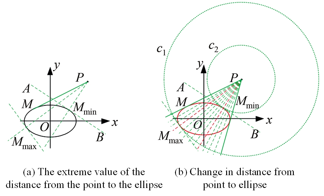
\[f\left( {{x_m}} \right) = |PM{|^2} = {m^2} + {n^2} – 2m{x_m} \pm 2n\sqrt {{b^2} – {{{b^2}} \over {{a^2}}}{x_m}^2} + {x_m}^2 + {b^2} – {{{b^2}} \over {{a^2}}}{x_m}^2.\tag{4}\] Let \(P\) be a point outside the ellipse, and let \(c_{1} and c_{2}\) be the tangent points to the ellipse, \(M_{\max}\) and \(M_{\min}\), respectively, as illustrated in Figure 7. The distance between the point and the ellipse is obviously increasing from \(P{M_{\min}}\), which is the minimum value, to \(P{M_{\max}}\), which is the maximum value, along the ellipse. This transition occurs both clockwise and anticlockwise, starting from the point \(M_{\min}\) and ending at \(M_{\max}\) [20].
The points \(M_{\max}\) and \(M_{\min}\) will be on both sides of the x-axis unless \(P\) is on the x-axis (that is, the co-planarity of the centre axes of the two cylinders, \(g_{1}\) and \(g_{2}\) ), and the distance of the points to the upper half-ellipse (on the x-axis) will be known to have at most one extreme point [21].
Based on the above reasoning, when calculating the shortest distance from a point to a partial ellipse, the following calculation can be used: assuming that the defining domain of the partial ellipse is \([s,t]\), the minimum value of the distance from the point to the complete ellipse is calculated as the corresponding \({x_{\min }}\), and the minimum value of the distance from the point to the complete ellipse is the lesser value of \(f({x_{\min }})\) if \(s\le x_{\min }\le t\), or the minimum value of the distance from the point to the complete ellipse if \(x_{\min } <s\). Otherwise, the minimum value of the distance from the point to the complete ellipse is the lesser value of \(f(s)\);Otherwise, the minimum is the smaller value of \(f(t)\). Note that \(f({x_{\min }})\) is a two-valued function [22].
The function derivation method or the geometrical relation \((AB \bot PM)\) can be used to determine the extreme value of \(f({x_{\min }})\), provided that PM takes the extreme value in order to solve the problem. In addition, if we take the extreme value and assume that AB is the ellipse’s tangent line, we find the following relationship:
\[\label{eq5} {k_{AB}} \cdot {k_{PM}} = {{{b^2}{x_m}} \over {{a^2}{y_m}}} \cdot {{n – {y_m}} \over {m – {x_m}}} = 1.\tag{5}\]
Also \(M({x_m},{y_m})\) is a point on the ellipse and from Eq. (5): \[\label{eq6} y_m^2 = {b^2} – {{{b^2}} \over {{a^2}}}x_m^2.\tag{6}\] Substituting Eq. (6) into Eq. (5) gives the quadratic equation for \({x_m}\): \[\label{eq7}\tag{7} {{c^4}{x_m}^4 – 2m{a^2}{c^2}{x_m}^3 + \left( {{n^2}{a^2}{b^2} + {m^2}{a^4} – \left. {{a^2}{c^4}} \right){x_m}^2 + 2m{a^4}{c^2}{x_m} – {a^6}{m^2} = 0} \right.},\] where \({c^2} = {a^2} – {b^2}\), and \(a>b\).
We simulated the debugged underground pipe culvert detection and positioning system in a straight, large-diameter PVC pipe section in order to verify the equipment’s detection accuracy and other functions. Table 1 displays the error calculation for each trajectory point.
| Track Type | Deflection angle | Trajectory error (10m) | 30m | 50m | 70m | 90m | 100m | Integral error(100m) |
| Straight path | 30 degrees northeast | 0.6m | 1.5m | 2.2m | 3.8m | 4.0m | 5.2m | 6.6m |
| 36 degrees northwest | 0.5m | 1.2m | 2.3m | 3.9m | 4.2m | 5.8m | 7.0m | |
| 48 degrees south by east | 0.2m | 1.2m | 3.4m | 4.2m | 5.1m | 6.8m | 7.3m | |
| 37 degrees south by west | 0.6m | 1.4m | 3.5m | 4.4m | 5.2m | 6.7m | 7.6m |
We choose the bending angles of the bellows for the test-30, 60, and 90 degrees-in order to better understand the accuracy of the plane position detection of the large-diameter bendable bellows. The trajectory point error calculation is displayed in Table 2.
Tests have confirmed that, in the situation of varied bending angles, the bending type path increases the angular error with an increase in bending angle.
| Track Type | Deflection angle | Actual measurement angle | Notes |
| Curve trajectory | 30° | 28°-31.5° | Statistical results of 5 actual measurements |
| 60° | 58.6°-62.5° | Statistical results of 5 actual measurements | |
| 90° | 90.3°-95.7° | Statistical results of 5 actual measurements |
Based on the measured data of three sets of underground pipe culverts of different scales in a certain city (the number of pipe segments included in data 1, 2 and 3 are 70, 153 and 531, respectively), the algorithm of this paper is compared with the results of collision detection using the three-dimensional intersection function of AutoCAD, ArcGIS and other softwares. When AutoCAD is used for collision detection, the cylinders are firstly generated according to the 3D coordinates of the measured pipe segments, radius and other geometric parameters, and then the 3D intersection (solid interference) function of the software is used to intersect the cylinders formed by all the pipe segments, and the collision is considered to be a collision if there is an intersecting part. In order to accomplish collision detection with ArcGIS, we must first use the pipe section’s radius as the buffer radius, create a cylindrical 3D buffer using the 3D buffer function, transform the buffer object into a 3D spatial cylindrical object, and then use the 3D intersection function to accomplish collision detection. The pipeline data corresponding to test data 2 and the outcomes of the collision detection are displayed in Figure 8.

Table 3, which displays the total number of collisions (including end-point and non-end-point collisions) and the number of non-end-point collisions detected by various algorithms, presents the collision detection statistics of the three sets of measured data of underground pipe culverts. Table 3 illustrates that while there is a minor discrepancy with the detection results of ArcGIS, the methodologies used in this paper are completely consistent with the results computed by AutoCAD. The output of the 2D collision method is displayed in the final column of Table 3. The algorithm projects the pipe axes horizontally first, and when they collide, the depth and radius of the colliding pipe points are utilised to determine whether or not a collision occurs. Currently, it is discovered that many real-world collisions in three dimensions cannot be identified, including the most evident scenario involving two pipe segments that are parallel to one another horizontally. The technique in this study is able to detect 285 collisions, indicating that the detection effect is extremely significant. Data 3 is the corrected data after the 2D collision check, therefore the number of collisions in 2D collision detection is 0.
| Test data | Total number of collisions/pair | Non endpoint collision count/pair | |||||
|---|---|---|---|---|---|---|---|
| Autoacd | ArcGIS | Our algorithm | Autoacd | ArcGIS | Our algorithm | 2D collision | |
| Data 1 | 90 | 90 | 90 | 45 | 45 | 45 | 12 |
| Data 2 | 290 | 290 | 290 | 176 | 176 | 176 | 25 |
| Data 3 | 630 | 632 | 628 | 286 | 2885 | 285 | 0 |
From the hardware side, we can see that the hardware facilities of the institutions are some basic hardware such as athletic fields and ball games, and not all schools have some hardware facilities such as swimming pools, which will limit the development of teaching contents to a certain extent. From the faculty side, it is found that there are few special teachers that students like, which will also limit the development of teaching contents [21].
Combined with Data 3, the 12 pairs of results not detected by ArcGIS are analysed, and there are three cases: 1) the two pipe segments are coincident at one end and the angle between the central axes is close to 180°, as shown in Figure 8(a); 2) the minimum spatial clear distance between the two pipe segments corresponding to the columns is close to 0, as shown in Figure 8(b); and 3) the overlap of the projected rectangles of the two pipe segments when the axes are separated is close to 0, as shown in Figure 8(c). as shown in Figure 8(d). The reason for not detecting the collision is that when the overlap of the two 3D pipe segments is very small, ArcGIS considers that the two segments do not intersect with each other.
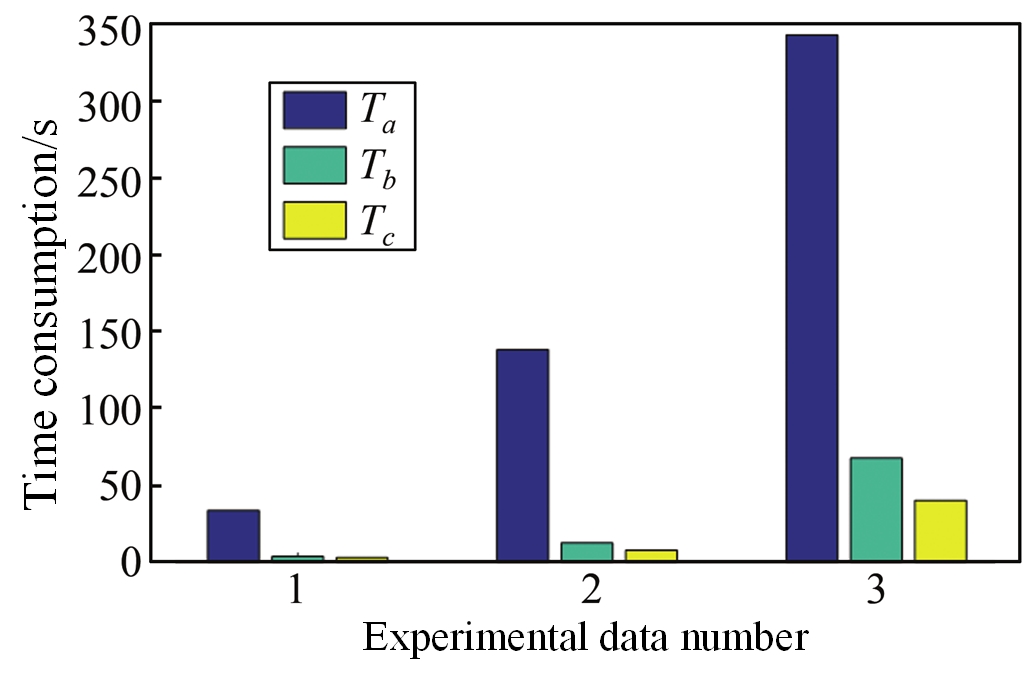
ArcGIS and AutoCAD are used to compare the effectiveness of the methodology in this study with other collision detection techniques. The techniques in this paper are based on Visual Studio 2010 C; the ArcGIS collision detection tool uses ArcMap’s 3D analysis tool; the AutoCAD collision detection algorithm is written in Visual Lisp and depends on the AutoCAD platform. The comparison test’s hardware configuration includes a 1.80 GHz CPU, 4 GB of RAM, 128 GB of SSD, and the Windows 10 operating system. The same three sets of underground pipe culvert data as in 3.1 are used for testing, and the efficiency statistics are shown in Table 4. \({T_a},{T_b},{T_c}\) represent the time consumption of ArcGIS, AutoCAD and this paper’s algorithms respectively, and \({T_a/T_c}\) and \({T_b/T_c}\) represent their corresponding efficiency ratios. Figure 9 shows the efficiency comparison of the three algorithms in the form of bar chart. From Table 4 and Figure 10, it can be seen that the efficiency of this algorithm is obviously higher than that of ArcGIS, which is several to ten times higher than that of ArcGIS, and the specific efficiency multiplier is closely related to the spatial relationship between the pipelines to be processed, and the algorithm of this paper has an obvious advantage over that of AutoCAD. The algorithm in this paper only requires the coordinates of the corresponding endpoints of the pipe segments and their diameter, and the spatial geometrical relationship between the pipe segments is directly used in the calculation. This simplifies the process of collision detection because it eliminates the need to build a 3D model in advance. The reason for this is that the algorithm in this paper contains many judgement statements, pipe segments with different spatial relationships will go through different processing procedures, and pipelines with simple spatial relationships will not be complicated [18].
| Test data | \({T_a/s}\) | \({T_b/s}\) | \({T_c/s}\) | \(T_a /T_c\) | \({T_b/T_c}\) |
|---|---|---|---|---|---|
| Data 1 | 32.584 | 3.365 | 2.586 | 12.985 | 1.232 |
| Data 2 | 138.264 | 13.254 | 7.658 | 19.257 | 1.658 |
| Data 3 | 342.458 | 65.325 | 38.564 | 8.565 | 1.655 |

The purpose of this study is to improve the positioning and detection precision of subterranean pipe culverts by proposing a pipeline collision detection method based on the projection of the common plumb line’s direction and the minimum distance calculation technique from a point to an ellipse. The pipeline collision detection method that utilises the projection of the common plumb line direction is a useful tool for efficiently identifying and locating underground pipe culverts in collision situations. By taking into account the projection position of subterranean pipe culverts in a vertical direction, the approach precisely calculates the collision scenario between pipelines, offering crucial technical support for the management and building of urban infrastructure. Secondly, the minimum distance calculation technology from the point to the ellipse has important application value in the detection and positioning of underground pipe culvert. Through the precise analysis of the ellipse shape and the position of the point, the minimum distance between the point and the ellipse can be accurately judged, which achieves the effective monitoring and positioning of the environment around the underground pipe culvert. Finally, this study also discusses the development trend and application prospect of underground pipe culvert detection technology.
Future underground pipe culvert detection and collision detection techniques will be increasingly sophisticated and accurate due to ongoing technological advancements, offering more dependable assistance for the maintenance and development of urban infrastructure.
This article does not have funding support.
The author declares no conflict of interests.