This paper analyzes the prediction model of enterprise human resource demand based on Internet of Things (IoT) technology and data mining technology. It also analyzes the impact of the company’s growth scale and other key factors on the demand for human resources, tries to establish a coupling factor model of enterprise development and economic benefits, and then analyzes and forecasts the enterprise’s personnel structure and quality structure. The experimental results show that the optimized human resource demand forecasting model integrates the advantages of the grey system model in data processing, can mine the inherent laws of unorganized data information, and provides a certain convenience for forecasting. Through the linear mapping and processing of sample data, the input and output reflect a kind of correlation, thus changing the fault tolerance of information, making the prediction in the calculation process more accurate, and its comprehensive accuracy can exceed 92.5%.
Since the 1980s, with the increasingly fierce market competition, enterprises have increasingly emphasized their ability to respond to the external environment and organizational change. During this period, human resources management regarded human resources as an important part of the whole system. During this period, a large number of scholars put forward new management theories [1]. Enterprises began to formulate corresponding human resource management strategies according to the development strategy. At this stage, “people-oriented and strategic incentive” is a popular human resource management method. In today’s uncertain society, full of challenges and opportunities, change is the premise for enterprises to survive and develop [2, 3].
According to statistics, the US human resources market currently has 160 million employees, and the expenditure amount of most enterprise personnel accounts for more than 40% of the company’s expenditure [4], which reflects the efforts and contributions of human resources employees to the enterprise and the importance of human resources management [5, 6, 7]. Human resources are concerned with the financial situation, turnover rate, personnel position matching and other conditions of the enterprise [8, 9, 10]. More and more companies use data to drive human resources management, including sales, return on investment, payback, turnover rate, employee satisfaction, assessment and evaluation results, etc. These various data stored in the enterprise can be used for analysis and research to obtain the human resources prediction results required by the enterprise. Enterprises store a lot of raw data, such as personnel structure, age, education, etc; Ability data, such as training, assessment, rewards and punishments, as well as potential data, work efficiency, income improvement level, etc; There are also some financial data, which belong to the data stored by the enterprise itself [11, 12]. Data is everywhere, and how to integrate and analyze, make decisions in the middle, and propose some optimization measures for the development of enterprises is the focus of human resources prediction [13, 14].
Therefore, this paper constructs a prediction method of enterprise human resource demand based on IoT technology and data mining technology, which provides a model hypothesis and reference basis for the prediction of human resources of related enterprises in China.
Human resource data is a huge and tedious dataset, which contains rich potential knowledge. More and more scientific and technological personnel try to use data mining methods to predict the future direction of human resources of enterprises. Human resource demand forecasting can not only integrate enterprise human resource data [14], but also improve the quality of analysis, and solve the problem of massive data mining. This chapter studies the main path of realizing human resource demand forecasting model by multiple linear regression analysis and data mining.
For specific prediction objects, if there is not a certain amount of data that conforms to the statistical law, it is not suitable to use multiple linear regression method for demand forecasting. On the basis of determining the statistical laws of independent variables and dependent variables, this chapter conducts multiple linear regression analysis to ensure the accuracy of human resource demand forecast. The standard equation of multiple regression is shown in Eq. 1.
\[\label{e1}\tag{1} \hat y = {b_0} + {b_1}{x_1} + {b_2}{x_2} + \cdots + {b_p}{x_p} + \varepsilon ,\] where, \(\hat y\) is predicted value of dependent variable; \({b_0}\) is regression constant; \(P\) is number of independent variables; \({b_i}(i = 1,2,…p)\) is regression coefficient, which represents variable change when other independent variables remain unchanged; \({x_i}(i = 1,2,…p)\) is regression factor, representing each independent variable [15]; \(\varepsilon\) is random error.
The human resource model uses the unbiased estimation of regression analysis to obtain the correct regression coefficient and regression constant by measuring \(n\) groups of independent observations ,\({y_k};{x_{k1}},{x_{k2}}, \cdots ,{x_{kp}},(k = 1,2, \cdots ,n)\) and finally obtains the fitted regression equation.
In the multiple regression model of enterprise human resources, the proportion of the variation of independent variables affected by the variation of dependent variables is determined by using the determination coefficient \({R^2}\), which is is shown in Eq. 2, and the closer \(R\) is to 0, the worse the model fitting degree is.
\[\label{e2}\tag{2} {R^2} = {{\sum\limits_{i = 1}^n {{{\left( {{{\hat y}_i} – \bar y} \right)}^2}} } \over {\sum\limits_{i = 1}^n {{{\left( {{y_i} – \bar y} \right)}^2}} }},\quad 0 \le R \le 1.\]
In the multiple regression model of enterprise human resources, with the increase of the number of samples, the determination coefficient \(R\) will increase, which is prone to the illusion that the more independent variables, the better the fitting effect, the correction \({R^2}\) is introduced as shown in Eq. 3.
\[\label{e3}\tag{3} {\rm Adjusted}{:} \quad{R^2} = 1 – {{\sum\limits_{i = 1}^n {{{\left( {{y_i} – {{\hat y}_i}} \right)}^2}} /(n – p – 1)} \over {\sum\limits_{i = 1}^n {{{\left( {{{\hat y}_i} – \bar y} \right)}^2}} /(n – 1)}}.\] Therefore, it is necessary to detect the linear relationship between variables by using the combination of \(F-test\) and \(t-test\) of linear hypothesis. The two inspection calculation methods are shown in Eqs 4 and [e5].
\[\label{e4}\tag{4} F = {{\sum\limits_{i = 1}^n {{{\left( {{{\hat y}_i} – \bar y} \right)}^2}} /p} \over {\sum\limits_{i = 1}^n {{{\left( {{y_i} – {{\hat y}_i}} \right)}^2}} /(n – p – 1)}}\ \sim F(p,n – p – 1).\]
\[\label{e5}\tag{5} {t_j} = {{{{\hat b}_{\rm{j}}}} \over {\sqrt {\sum\limits_{i = 1}^n {{{\left( {{y_i} – {{\hat y}_i}} \right)}^2}} /(n – p)\sqrt {\sum\limits_{i = 1}^n {{{\left( {{y_i} – {{\hat y}_i}} \right)}^2}} /(n – p – 1)} } }}\ \sim t(n – p – 1).\]
Based on the analysis of key factors, quantitative analysis mainly based on regression prediction method, supplemented by qualitative analysis such as expert discussion method, is used to build demand prediction models from three aspects of the total amount, structure and quality of human resources of the pilot company, so that the pilot company can formulate human resources planning more scientifically [16].
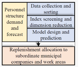
First, for the control of total employment, through the analysis of business growth on employment demand, use mathematical statistics to determine the impact of many major factors on the total employment, combine the enterprise’s business management strategy, consider the impact of production efficiency improvement on employment demand, and build a total demand forecasting model that takes into account business development and efficiency improvement; On this basis, the predicted number of supplementary personnel in each year and each discipline will be allocated to the subordinate prefecture companies and relevant work areas, as shown in Figure 1.
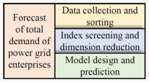
First, distinguish the core level of the business, further divide the corresponding employment types, and analyze the number of long-term employees in each subordinate company and work area. The quality requirements of new long-term employees include many aspects, such as education background, graduation colleges and disciplines. Through the analysis of these aspects, the quality demand forecast of new long-term employees is formed; Then analyze the staffing rate of each discipline in subordinate units. Since the pilot company belongs to this enterprise, it is necessary to distinguish the importance of each discipline for the safety production association, and consider setting the elasticity coefficient of each discipline. At the same time, according to the development requirements of the pilot company, the status of each subordinate unit is divided, so as to analyze the priority of recruitment, further clarify the priority of recruitment of new long-term employees in each subordinate unit, and finally complete the model construction of recruitment quality requirements, as shown in Figure 2.
Then, the calculated error ratios \(C\) and \(P\) are described by Eq. (6):
\[\label{e6}\tag{6} C = {{{S_2}} \over {{S_1}}},P = P\left\{ {|{q^{(0)}}(k) – {{\bar q}^{(0)}}\mid < 0.674{S_1}} \right\},\] when \(p>{p_0}\), the minimum error rate of the prediction model indicates that it is a qualified model, and vice versa. To sum up, the grey model of enterprise human resource demand prediction does not require a large number of samples in the prediction process, nor does it need to consider whether the data obey certain probability distributions [17]. Because the grey prediction model can mine the potential laws of data, the essence of things can be reflected through the establishment of some dynamic differential equations, as shown in Table 1.
| Grade index | Relative error $$\varepsilon (k)$$ | Accuracy $$P^\rm{a}$$ | Posterior error ratio $$C$$ | Error probability $$P$$ | Correlation degree $$r$$ |
| Good | 5%95% | 0.35 | 0.95 | 0.95 | |
| Qualified | 10% | 90% | 0.65 | 0.85 | 0.85 |
| Reluctantly | 15% | 85% | 0.75 | 0.75 | 0.75 |
| Unqualified | 25% | 75% | 0.85 | 0.65 | 0.65 |
Based on the above prediction models for the total amount, structure and quality demand of human resources, a prediction model for the demand of human resources is established to control the total amount of labor, gradually balance the allocation of labor, and constantly optimize the staff.
In order to carry out the research on human resource demand prediction of scale enterprises, we choose the typical scale enterprise as the research object. Company A was founded in 2000 and Company B was founded in 2010. It is a leading enterprise in related industries in China and the first design and research center for related products in China.
In the research, we mainly interview and understand the business managers in different departments of the enterprise, as well as the human resources department and the senior management of the enterprise, and analyze some human resources related data according. In the process of specific research and data collection, the main arrangements are as follows: First, conduct overall research on enterprises A and B. In the research activities, we mainly communicate with the senior managers of the enterprise, and let the HR department cooperate to carry out the actual research activities after obtaining their permission. Then a special research lady coordinated with the human resources department of the enterprise and proposed specific research requirements, so that the enterprise could be the human resources department to make some research arrangements. Second, in the process of enterprise research, we selected ten main functional parts of the enterprise, as well as regional sales branches and business departments under the enterprise [18].
In the process of investigation, a systematic data collection table was prepared for the cooperation of the human resources department. Third, in the process of research, collect and sort out the literature related to human resource demand forecasting, so as to lay a good experimental foundation for the whole forecasting process. During data preprocessing, use scattered regression of business volume, production level, human resource flow rate, production volume, employee growth rate, R\(\&\)D capital investment rate, employee satisfaction and other indicators for selection, such as Eqs (7) and (8):
\[\begin{aligned} \label{e7} {e_c} &= {w_1}{e_1} + {w_2}{e_2}. \end{aligned}\tag{7}\] \[\begin{aligned} var\left( {{e_c}} \right) &= E\left( {e_c^2} \right) – {\left[ {E\left( {{e_c}} \right)} \right]^2}\notag\\& = E\left( {e_c^2} \right)\notag\\& = var\left( {{w_1}{e_1} + {w_2}{e_2}} \right) \end{aligned}\] \[\begin{aligned} \label{e8} &= w_1^2var\left( {{e_1}} \right) + w_2^2var\left( {{e_2}} \right) + 2{w_1}{w_2}cov\left( {{e_1},{e_2}} \right). \end{aligned}\tag{8}\]
In our data set, we consider many internal factors of enterprise HR forecast, such as production demand, performance indicators or other liquidity data. The data set indicator system is shown in Table 2.
| Secondary indicators | Third level indicators |
|---|---|
| Enterprise scale | Total assets |
| Net assets | |
| Production demand Total | enterprise output value |
| Outcome indicators | Profit |
| Sales revenue | |
| Labor cost trend | Comparison between enterprise wages and regional industry wages |
| Average wage level | |
| Technical elements | Labour productivity |
| Training needs | Training input |
| Mobility of employees in each type of work | Promotion ratio |
| Miner trends | Attendance |
| Degree of brain drain | Resignation rate |
| Retirement ratio |
Key indicators refer to the indicators with large weight in the prediction of enterprise human resource demand. Different enterprises or enterprises in different stages of development have different key indicators for human resource prediction. Grey relational analysis can objectively delete and select key indicators. Grey relational analysis specifies the quantitative comparison and description of the relative changes over time between systems or among various factors in the system during the development process. According to the information disclosed by listed companies and enterprise research information, the relevant data of enterprises A and B since 2000 are analyzed by grey correlation analysis [3]. \({X_i} = \left\{ {{x_i}(1),{x_i}(2), \ldots ,{x_i}(8)} \right\},i = 1,2,3 \ldots ,15\), representing the series of the third level indicators from 2000 to 2020. The sequence (9) obtained by averaging is used as the final output sequence. As Table 3 for data extraction.
\[\label{e10}\tag{9} {x_i} = {{{x_i}} \over {\overline {{X_i}} }}{x_i}(1),{x_i}(2), \cdots ,{x_i}(8)\} ,\quad\text{where}\quad{\rm{ }}\overline {{X_i}} = {1 \over 8}\mathop \sum \limits^8 {x_i}.\]
| Data extraction indicators | Specific gravity extracted |
|---|---|
| Highly educated personnel | \({Y_1}({Y_1} = {Y_{11}})\) |
| Labour productivity | \({Y_2}({Y_2} = {Y_8})\) |
| Enterprise net asset value | \({Y_3}({Y_3} = {Y_2})\) |
| Managers in the enterprise | \({Y_4}({Y_4} = {Y_9})\) |
| Scientific and technological personnel in enterprises | \({Y_5}({Y_5} = {Y_{10}})\) |
After the model is established, we need to conduct systematic experiments and accuracy analysis on the prediction model. System dynamics is a relatively mature model with more general validation rules. First, the model should be able to truly reflect the situation of the research object in real life, which is generally an intuitive test. Secondly, structural inspection, accuracy test and sensitivity test are also required to determine the feasibility of the model.
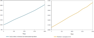
The first part is the structural test, which is mainly to test whether the model establishment is obviously sensitive to the changes in the initial settings. Generally, the asynchronous length is used for testing. The internal logic of the structure inspection is that if the change trend of the simulated results of the model remains roughly consistent under the conditions of different value settings for the simulation step size (DT, in this model, refers to time), the model can be considered stable, that is, it has passed this inspection [12]. In this paper, some indicators (such as family culture, education and entertainment expenditure, residents’ consumption level, added value of industry or other related industries, and total employment of the company) are selected as observation objects for verification, and four simulation step sizes are set. The four simulation step size modes are: Current step size is 1, DT1 step size is 0.5, DT2 step size is 0.25, and DT3 step size is 0.125. The model operation simulation is carried out in these four modes. The operation results show that under different simulation step sizes, the change trend of the operation results of the selected factors is basically unchanged, with good consistency, as shown in Figure 3. It can be seen that the model established in this paper is not sensitive to changes in initial settings, and this model has strong stability. Therefore, this model is considered to have passed the structural test.
The second part is precision inspection. The measurement accuracy is the amount of error between the prediction result and the real value after the model is established. This paper selects 2010 as the initial time for model simulation, and compares it with the real original data to verify whether they are consistent. Of course, there are differences between the model simulation results and the actual values. In view of the objective existence of factors such as the omission of information inside the system caused by the white box modeling method of the system dynamics model itself and the fitting of variable equations cannot reach 100%, we generally believe that the simulation error is within the acceptable range if it does not exceed 10%. Two variables, total population in 2010-2018 and total labor volume in China, are selected for precision test, as shown in Table 4:
| Particular year | Electricity sales (100 million Kw*h) | Wage growth rate (%) | R$$\&$$D investment rate (%) | Number of personnel (person) | Predicted value (person) | Error |
| 1 | 49.3 | 10 | 1 | 3040 | 3055 | -0.54% |
| 2 | 53.7 | 6.2 | 1.43 | 3005 | 3000 | 0.84% |
| 3 | 58.2 | 11.4 | 0.9 | 3015 | 3010 | -0.08% |
| 4 | 63.2 | 0.4 | 1.54 | 2905 | 2910 | -0.22% |
| 5 | 71.6 | 0.5 | 1.11 | 2875 | 2880 | -0.43% |
| 6 | 81.8 | 8 | 1.6 | 2830 | 2840 | 0.16% |
| 7 | 91.7 | 7.7 | 1.4 | 2805 | 2770 | 0.92% |
| 8 | 100.7 | 12 | 1.84 | 2670 | 2680 | -0.84% |
| 9 | 110.9 | 11 | 1.9 | 2645 | 2655 | 0.46% |
| 10 | 118 | 10.8 | 1.33 | 2600 | 2610 | 0.35% |
| 11 | 123.99 | 10.5 | 1.52 | – | 2565 | – |
| 12 | 130 | 10.7 | 1.57 | – | 2525 | – |
| 13 | 134.7 | 12 | 1.8 | – | 2495 | – |
The third part is the empirical test results of the model. The operation results of the enterprise human resource demand forecasting subsystem are shown in Table 5. The error between the operation results of the model and the actual results is small. The forecast results of China’s labor force population show that China’s labor force population is gradually increasing from 784.885 million in 2010 to 812.88 million in 2018, with an error less than 1% from the original data.
| Particular year | Population of working ages | Raw data | Error | Employed population in electric heating industry | Raw data | Error |
| 2010 | 78488.1 | 78388 | -0.00128 | 212.88 | 208.3 | -0.01763 |
| 2011 | 78804.7 | 78579 | -0.00286 | 207.823 | 220.7 | 0.060988 |
| 2012 | 79063.4 | 78894 | -0.00214 | 204.314 | 223.2 | 0.093425 |
| 2013 | 79340.4 | 79300 | -0.00051 | 200.03 | 203.0 | 0.015948 |
| 2014 | 79638.5 | 79690 | 0.000644 | 195.328 | 196.7 | 0.008057 |
| 2015 | 79988.6 | 80091 | 0.001283 | 189.317 | 182.8 | -0.03548 |
| 2016 | 80361.3 | 80694 | 0.004143 | 182.755 | 179.6 | -0.01616 |
| 2017 | 80845.5 | 80686 | -0.00197 | 173.366 | 162.9 | -0.0593 |
| 2018 | 81288.0 | 80686 | -0.0074 | 165.357 | – | – |
Through the model running simulation, the company’s human resource forecast data is obtained. The company’s human resource model simulation results are shown in Tables 6 and 7. The experimental results show that the simulation results of the model are consistent with the actual situation. From the total number of employees of Company A, the error of this prediction model is only 0.96%. The simulation results, like the original data, also have a trend of rising first and then falling, and the overall model is relatively good. The error between the predicted results and the actual results of the graduate students and above is slightly large, mainly because the talents at this level belong to high-level talents, and the change law is not obvious [19]. The model prediction is for the first consideration, resulting in a large error of individual values, but still within the controllable range of the model prediction error.
| Particular year | Total number of employees | Raw data | Error | High school and below | Original | Error |
| 2010 | 26550 | 26805 | 0.96% | 12212.6 | 12314 | 0.85% |
| 2011 | 27773.6 | 28033 | 0.94% | 11968.9 | 12215 | 2.04% |
| 2012 | 30281 | 30657 | 1.24% | 12233.3 | 12143 | -0.76% |
| 2013 | 30842.2 | 31093 | 0.81% | 11304.4 | 11555 | 2.22% |
| 2014 | 28039.7 | 28333 | 1.05% | 10489.6 | 10147 | -3.25% |
| 2015 | 27723.3 | 27745 | 0.07% | 9440.24 | 9699 | 2.72% |
| 2016 | 27077 | 27089 | 0.03% | 8458.97 | 8585 | 1.48% |
| 2017 | 26422.6 | 26390 | -0.13% | 8045.5 | 7919 | -1.58% |
| 2018 | 25536.6 | 25550 | 0.05% | 7263.17 | 7235 | -0.42% |
| Junior college predicted value | Original value | Error | Undergraduate forecast value | Undergraduate | Error | Postgraduate or above | Estimate | Error |
| 7890.44 | 7973 | 1.04% | 6155 | 6476.25 | 5.22% | 368 | 414.116 | 12.61% |
| 8418.13 | 8484 | 0.78% | 6919 | 7373.33 | 6.57% | 422 | 490.077 | 16.13% |
| 9491.66 | 9606 | 1.20% | 8366 | 8285.56 | -0.96% | 537 | 541.671 | 0.09% |
| 9742.95 | 9786 | 0.44% | 9128 | 9086.55 | -0.45% | 620 | 620.25 | 0.04% |
| 8550.26 | 8885 | 3.91% | 8676 | 9651.08 | 11.24% | 624 | 740.42 | 18.66% |
| 8427.1 | 8546 | 1.41% | 8866 | 8508.44 | -4.03% | 636 | 618.555 | -2.74% |
| 8164.43 | 8120 | -0.54% | 9575 | 8617.6 | -9.99% | 805 | 643.855 | -20.0% |
| 7886.24 | 7831 | -0.70% | 9828 | 9669.23 | -1.62% | 814 | 775.233 | -4.76% |
| 7515.77 | 7472 | -0.58% | 10078 | 10266.6 | 1.87% | 809 | 860.244 | 6.33% |
It can be seen that Table 8 and Figure 4 are obtained through model simulation. According to the table below, the model predicts that the number of employees in other companies will gradually decrease from 2129300 in 2010 to 1557000 in 2018. The error with the actual situation is less than 4%, and the running results of the model are reliable and reproducible [6].
| Particular year | Employed population in electric heating industry | Total number of employees | Number of employees in other companies | Error ratio |
| 2010 | 212.88 | 2.6552 | 212.934 | -0.01288 |
| 2011 | 207.822 | 2.7777 | 213.471 | -0.04056 |
| 2012 | 204.315 | 3.0281 | 214.242 | -0.06343 |
| 2013 | 200.04 | 3.0844 | 214.375 | -0.08724 |
| 2014 | 195.322 | 2.8036 | 186.826 | 0.029144 |
| 2015 | 189.316 | 2.7725 | 182.116 | 0.023395 |
| 2016 | 182.755 | 2.7075 | 175.468 | 0.025055 |
| 2017 | 173.367 | 2.6425 | 162.955 | 0.044786 |
| 2018 | 165.356 | 2.5539 | 155.696 | 0.042977 |
Factor analysis is carried out for the human resource demand subsystem of the company, taking the total number of employees of the company as the observation variable, changing other influencing factors, and obtaining the data of influence degree, as shown in Figure 5. It can be seen from the table below that there are 13 positive factors and 11 negative factors affecting the total number of employees. From the perspective of impact degree, the company’s human resource capacity ranked first, with the impact degree of 13%; The second place was the enthusiasm of employees, with an impact of 9.66%; The third is the total human resource capacity of the company, with an impact of 9.43%; The fourth is employee compensation payable, with an impact of 9.41%; The fifth is the company’s labor volume, with an impact of 8.92%.
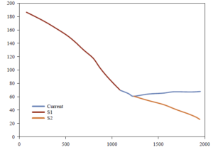
Then, through the fitting and forecasting analysis of the model, the influencing factors of the supply and demand difference of enterprises A and B are obtained. As Figure 6 for details.
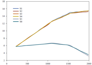
According to the Figures 5 and 6, there is a difference between the total supply and demand of China’s industry or other related industries in the future according to the prediction results of the model. There is a large difference between scenarios S1, S2, S5 and S6, and the difference is gradually increasing, indicating that the supply of talent in the future market is greater than the demand. Through specific scenario settings, the natural population growth rate of S2, S3, S5 and S6 in these four scenarios is at a low growth rate, while the human resource capacity is at a high growth level. In scenarios S1, S2 and S5, the difference between total supply and total demand will rise to a small extent and then decline in 2021. There will be a further downward trend in the future. At this time, the total demand may be greater than the total supply. In these four scenarios, the natural population growth rate and the company’s human resource capacity are at a high development rate. In other words, the calculation results of this model show that due to the uncertainty of future development, the company should formulate talent support strategies for different development trends.
Data mining technology can make full use of the enterprise’s own data, greatly improve the development and operation level of the enterprise, and use it to expand business, so that enterprises can better improve themselves, serve the society, and serve users. Based on the theory of association between things in data mining, and in this paper, data mining and human resources are coupled to build a demand forecasting system. Finally, through linear mapping and sample data processing, the input and output reflect a kind of correlation, thus changing the fault tolerance of information, making the prediction in the calculation process more accurate. Its comprehensive accuracy can exceed 92.5%. The relevant influence factors of the model include the total number of employees, human resource capacity, salary expectations, etc.
No funding is available for this research.
The author declares no conflict of interests.