
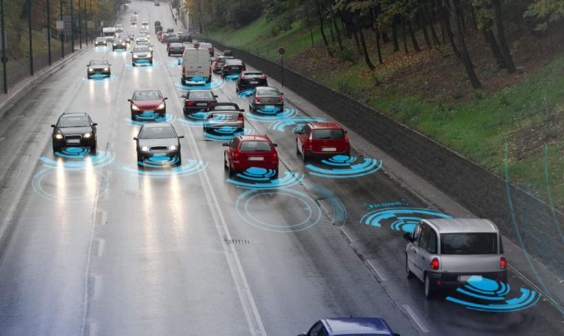
As people’s spending power increases, more and more people choose cars as a means of transportation for travel. However, because of the irregular operating habits of drivers of traditional cars, car accidents can occur and the personal safety of passengers is not guaranteed. Due to the development of artificial intelligence, 5G communication and other technologies, driverless vehicle technology has been developed and applied to the ground [1].
As early as the 1950s, foreign researchers geared toward driverless vehicle technology research, while major traditional car companies and technology well-known companies have invested a lot of research and development funds into the driverless field. After a long period of technical exploration and accumulation, they were all able to self-research their own driverless cars successfully. In terms of unmanned vehicle development policy, DARPA, a research and planning agency under the U.S. Department of Defense, held three driverless car competitions from 2004 to 2007 in order to develop unmanned vehicle technology, and the success of the competitions has given a good impetus to driverless technology [2].
In 2010, Google in the United States invested a lot of research and development funds to carry out the research and development of unmanned vehicle technology, and due to Google’s long-term unmanned vehicle technology accumulation, it is able to produce high-performance driverless cars. Until now, companies such as Tesla, Uber, Apple, and General Motors have also been developing their technologies in the competition of driverless cars, and these companies have invested heavily in research and development and achieved good results [3].
In the 1990s, China’s National University of Defense Technology developed the unmanned vehicle CITAVT-I, which is the real meaning of unmanned vehicle in China. In 2003, China’s Tsinghua University independently developed the unmanned vehicle THMR-V, and later in 2006, Tsinghua University, the development of the unmanned vehicle Red Flag HQ3 was successful. China has experienced more than a decade of catching up, and has actively carried out research on driverless technology in various universities, high-tech enterprises, and various research institutions, making domestic driverless technology from nothing to something to a leading position [4]. In 2015, Baidu’s unmanned car completed tests in an industrial park in Beijing, realizing complex driving actions, being able to switch freely between different road scenarios, and being able to travel at a 100km/h maximum speed. In 2018, Baidu’s unmanned vehicle division, together with the Golden Dragon Bus Group, launched an unmanned bus called “Apolong” for mass production and sales.
Since then, domestic driverless technology has developed unprecedentedly, and major companies have produced and developed numerous driverless cars, such as Drip Hail, Meituan, Beijing Baidu and other companies to the public, providing unmanned cab services, and in 2021, BAIC Group adopted Huawei’s driverless system solution and jointly launched the commercial Polar Fox Alpha unmanned vehicle, and domestic companies such as Xiaomi, Jingdong Group, Alibaba Group, etc., which have strong technological strength, have increased their commitment to the development of driverless cars, Alibaba Group, etc., have increased their R&D efforts on commercial unmanned vehicles, and unmanned vehicle products of various functions have been launched, such as unmanned express transport logistics vehicles, Jingdong express delivery vehicles, road sweepers, etc. In addition, emerging unmanned vehicle manufacturers such as Azure, Xiaopeng, Jidu, Ideal and Pony Smart have risen and their product quality has been recognized both at home and abroad. More and more unmanned vehicles are getting commercialized into the life of the general public, and it is certain that the driverless technology system is becoming more and more mature [5].
Even so, there are still many problems in path planning and trajectory tracking of driverless vehicles, and many crashes have occurred in commercial unmanned vehicles so far in 2018. in March 2018, the U.S. company Uber unmanned vehicle knocked down and killed a woman riding a bicycle across the road, resulting in the first case of “unmanned vehicle crash that killed a person” worldwide [6]. In 2021, in Zhengzhou, Henan Province, a Tesla Model 3 car lost its brakes [7, 8] and rear-ended the car in front of it, resulting in a serious crash that nearly killed it. These traffic accidents are equipped with advanced sensing devices and do not have hardware functional defects, which are attributed to the immaturity of unmanned vehicle local path planning obstacle avoidance and control system technology.
In addition, the current major car manufacturers to the unmanned technology to invest huge research and development funds, unmanned car vehicle equipment LIDAR, camera, industrial control machine prices account for a large proportion of the total car cost. However, as the production process of chips and radar is improved, the price of hardware equipment is getting lower and lower, and the low-cost embedded computing platform is getting more and more favored, but its computing resources still have a gap compared with the arithmetic power of traditional industrial control machines, directly transplanting the existing path planning and trajectory tracking to the embedded platform, the real-time planning and trajectory accuracy of its unmanned system is difficult to meet the requirements. Therefore, with the limited computing resources, it is an urgent problem to ensure the real-time performance of UAS planning and the accuracy of trajectory tracking.
With the rapid development of AI technology, the embedded computing platform GPU algorithm power is gradually becoming higher, and the driverless complete system is getting smaller and smaller, occupying the space of the vehicle. Driverless technology is a combination of AI technology, laser technology, 5G communication, multi-sensor information fusion and other technologies that enable rapid commercial mass production of driverless cars [9, 10]. Path planning is an important part of the driverless car system, enabling the planning of a path that ensures the driverless car reaches its target mission based on the current perceived obstacles [11]. Local path planning collects and processes information in constantly changing road conditions and corrects the path based on actual environmental information, and that path is able to avoid all obstacles [12, 13].
Domestic automakers and technology companies are late to enter the unmanned vehicle field, but have worked tirelessly to conquer new technologies [14]. One of the first companies to develop unmanned vehicle technology within China, Baidu has accumulated considerable experience and core technologies, and in 2017, Baidu’s unmanned vehicle division announced Apollo, an open-source autonomous driving platform that helps researchers and developers, as a huge contribution to the industry’s unmanned vehicle research [15, 16].
In 2020, Baidu launched Apollo Go cab service in Beijing, where users can make reservations to experience Robotaxi on Baidu Maps. 2021, Huawei and BAIC jointly developed and launched the Extreme Fox car [17, 18], which can not only sense sudden cars and stop in time in self-driving mode, but also drive and stop in many narrow and complex road conditions where pedestrians and cars mix freely. Huawei is able to self-research in-vehicle chips, in-vehicle communication devices, and various sensors, which can further reduce the cost of the whole vehicle [19]. In addition, Azure Automotive, Drip, Pony Smart, and Xiaopeng Automotive have all produced corresponding driverless cars.
Foreign research on driverless technology is relatively early, and as early as 2012, the Google Unmanned Car developed by Google Technologies in the United States was successfully tested on real traffic roads, and the U.S. Department of Motor Vehicles issued legal motor vehicle licenses for the unmanned cars developed and produced by Google Technologies. In this regard, Tesla’s driverless Autopilot assistance system, which mainly uses a front industrial monocular camera to sense road information in front of the car, identify lane lines, ultrasonic radar ranging, GPS positioning, etc., the system achieves lightweight deployment in Model series cars and uses pure vision for obstacle avoidance and path planning [20]. In addition, in 2015, the University of Tokyo, Japan, together with Tier IV, launched the Autoware project [21], which, with the release of the open source Autoware AI, is the world’s first open source software for unmanned vehicle driving technology, providing a platform for researchers and unmanned vehicle enthusiasts, to learn unmanned vehicle technology [22, 23].
In general, scholars at home and abroad have studied more path planning methods for vehicles in urban road network environment, and their research results are quite abundant, especially the estimation model of road section travel time, the construction of dynamic road resistance function based on road section travel time prediction, and the dynamic path planning algorithm for driverless vehicles in the existing urban road network environment have achieved more substantial results. On the contrary, relatively little research has been conducted by domestic and foreign scholars on the screening of alternative driving sections for driverless vehicles, the path planning of driverless vehicles in the road network environment with driverless lanes, and the reservation and allocation mechanism of right-of-way. The existing research results on traditional vehicle path planning are richer and can well provide better ideas and theoretical support for the topic selection, methods, framework conception and algorithm improvement of the thesis.
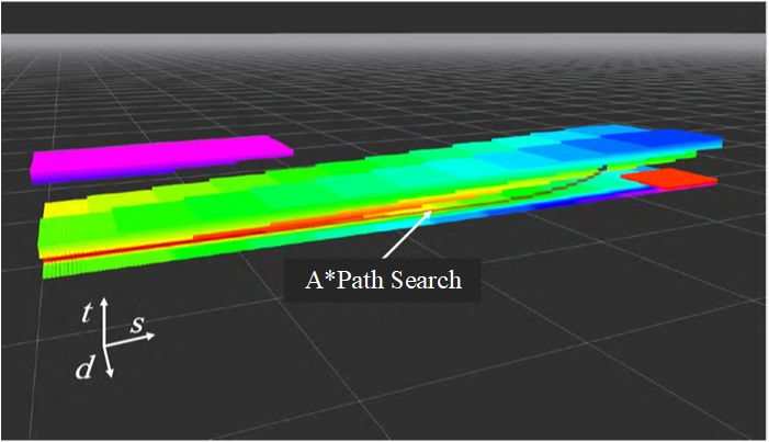
The algorithm system described in this paper is shown in Figure 1, which mainly contains three modules: spatiotemporal navigation map construction, front-end path search and trajectory optimization based on B-sample curve. Firstly, based on the main vehicle state information (which includes position, speed, direction, etc.) from the perception module, the motion information of the surrounding dynamic vehicles and the road structure information, the local 3D spatiotemporal occupation raster map of \(\left( {s,d,t} \right)\) in the fence net coordinate system is constructed by trajectory prediction of the surrounding dynamic vehicles, and the Euclidean Signed Distance Fields (ESDF) [24]. Based on our team’s completed spatiotemporal lane gap decision (a comprehensive analysis of road traffic conditions, a lane gap decision topology is constructed, and the optimal decision topology path is selected as the real-time decision result for the driverless car, which is mainly used to guide whether and how to change lanes (which gaps to pass in turn). The raster path is obtained by local target point selection and A* path search for the decision gaps. The raster path points are sampled as the initial control points of the B-sample curve, and a uniform B-sample curve is constructed, and the control points are optimized non-linearly based on the Euclidean signed distance field to obtain a vehicle kinematic constrained trajectory.

In the high-speed road environment, the vehicle does not perform any reversing operation, therefore the local map used in this paper method only considers the 50 m range area in front of the driverless car under the Frene coordinate system, and the included time dimension range is 0 5 s. As shown in Figure 2, the vehicle perception results are mapped to the local coordinate system, and the main vehicle position is always kept fixed (marked in black in Figure 2).

Since the focus of this paper does not include vehicle trajectory prediction, for the surrounding dynamic vehicles, we investigate the use of linear prediction method to estimate the motion state of the surrounding vehicles, so as to obtain a 3D spatial occupation raster map as shown in Figure 3, with a map resolution of 0.02m. The time dimension is from the current moment to the next 5 s, in order to infer the motion distribution of the surrounding vehicles within 5s. The difference in vehicle speed is presented as the occupation The difference in velocity of the vehicles is presented as a difference in the slope of the raster points in the positive direction of the time axis. As shown in Figure 3, vehicle 1 has a higher speed compared to vehicle 4, and the sequence of raster points for vehicle 1 has a greater slope along the time axis in Figure 3.
The role of 3D occupancy raster is to provide feasible search space for the front-end path search module, while for the back-end trajectory optimization module, to ensure the safety and feasibility of the trajectory, it is necessary to constrain the position of the control points of the trajectory, which includes the distance from the obstacles. As the 3D occupied raster map cannot provide distance information directly, this paper describes the distance information of any point in the 3D space from an obstacle by constructing a Euclidean symbolic distance field in the 3D space and querying the distance and gradient information of the obstacle. The application of the Euclidean symbolic distance field is important for online motion planning of robots. The FIESTA map system was proposed in[25] in 2019 to incrementally build ESDF maps. The FIESTA system achieves updating as few map nodes as possible within the framework of a breadth-first search algorithm by introducing two separate update queues for inserting and deleting obstacles, using indexed data structures and bidirectional chaining tables for ESDF map maintenance. As shown in Figure 4, the ESDF map in 3D space at t = 0, 1, 2, 3, 4 s is shown on the right. Where the main vehicle is located in the third lane, the distance information from the obstacle at any point can be quickly obtained according to the constructed ESDF map for back-end trajectory optimization.

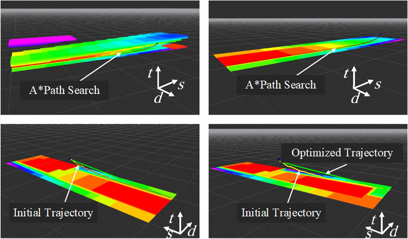
Based on the 3D spatiotemporal map construction and the spatiotemporal gap decision algorithm already completed by our team, local target points \(g\left( {s,d,t} \right)\) in 3D space and 3D occupied raster maps can be obtained. Then, the A* search algorithm is used to search the path from the main vehicle node to the target point: where the heuristic function used is the Euclidean distance function, described as the Euclidean distance of the current node from the target point \(d\). As shown in Figure 5, in the process of driving on high-speed roads, the vehicle driving cannot turn around or reverse, so in conducting the path search, the search direction is restricted to the positive direction of the \(s\) and \(t\) dimensions to reduce the number of visits during the search number of nodes and shorten the A* search time.
A B-sample curve is a linear combination of B-sample basis functions (all the spline functions on a given interval forming a linear space), as shown in Figure 6.
Let \(\left\{ {{Q_0},{Q_2},…,{Q_N}} \right\}\) have a total of\(N + 1\) control points and a node vector \(U = \left\{ {{u_0},{u_2},…,{u_m}} \right\}\), which is used to define a \(K\) order (\(N + 1\) times) spline curve, where \(k \geqslant 1,m = N + k\) must be satisfied, then the order spline curve is defined as Eq. (1):
\[\label{e1}\tag{1} p(u)=\left[Q_0, Q_2, \ldots, Q_N\right]\left[\begin{array}{c} B_{0, k}(u) \\ B_{1, k}(u) \\ \vdots \\ B_{n, k}(u) \end{array}\right]=\sum_{i=0}^N Q_i B_{i, k}(u) ,\] where \({B_{i,k}}\left( u \right)\) is the \(i\)-th order \(B\) sample basis function corresponding to control point \({Q_i}\), defined as Eq. (2):
\[\label{e2}\tag{2} \begin{aligned} & \mathbf{B}_{i, 1}(u)=\left\{\begin{array}{l} 1, \quad u_i \leqslant u \leqslant u_{i+1}, \\ 0, \quad \text { other }. \end{array}\right. \\ & \mathbf{B}_{i, k}(u)=\frac{\left(u-u_i\right)}{u_{i+k-1}-u_i} \mathbf{B}_{i, k-1}(u)+\frac{\left(u_{i+k}-u\right)}{u_{i+k}-u_{i+1}} \mathbf{B}_{i+1, k-1}(u), u_{k-1} \leqslant u \leqslant u_{N+1}. \end{aligned}\]
The \({\bf{B}}\)sample trajectory can be parametrized by time \(t\), where \(t \in \left[ {{t_k},{t_{m – k}}} \right]\). For a uniform \({\bf{B}}\) sample curve, the value \(\Delta t\) is the same for each node span \(\Delta {t_j} = {t_{j + 1}} – {t_j}\). Therefore, for the local start point \(\left( {{s_0},{d_0},{t_0}} \right)\)and the local target point\(\left( {{s_g},{d_g},{t_g}} \right)\), the nodal span is defined as \(\Delta t = \left( {{t_g} – {t_0}} \right)/\left( {m + 1} \right)\).
To constrain the velocity and acceleration within the specified limits and to penalize velocities and accelerations that exceed the maximum allowed value \({v_{\max }},{a_{\max }}\), the overspeed evaluation function is designed as follows:
\[\label{e3}\tag{3} F_v\left(v^p\right)= \begin{cases}\left(v^{p 2}-v_{\max ^2}\right)^2 &\qquad v^{p 2}>v_{\max ^2}, \\ 0 & \qquad v^{p 2} \leqslant v_{\max ^2},\end{cases}\] where \(p \in \{ s,d\}\), the super-acceleration evaluation function is of the same form. Based on both, velocity and acceleration cost functions \({f_v}\) and \({f_a}\) are defined to penalize control points where velocity and acceleration are not feasible, in the following form:
\[\label{e4}\tag{4} \left\{\begin{aligned} & f_v=\sum_{\substack{p \in \\ \{s, d\}}} \sum_{i=2}^{N-3} F_v\left(V_i^p\right), \\ & f_a=\sum_{\substack{p \in \\ \{s, d\}}} \sum_{i=1}^{N-3} F_a\left(A_i^p\right). \end{aligned}\right.\]
The curvature cost function is defined as Eq. (5):
\[\label{e5}\tag{5} {f_\kappa } = \sum\limits_{i = 1}^{N – 3} {{{\left( {\kappa {{\left( {{{\bf{Q}}_i}} \right)}^2} – {\kappa _{\max }}^2} \right)}^2}},\] where \(\kappa \left( {{{\bf{Q}}_i}} \right)\) represents the curvature at \({{\bf{Q}}_i}\), which needs to be converted to a Cartesian coordinate system for the trajectory curvature cost calculation.
Figure 7> shows the initial control points obtained by first sampling the path points from the A* search and uniformly distributing the time to obtain the uniform spline curve (yellow trajectory in Figure 7). The optimization problem of Eq. (4) is solved using the NLOPT-LD-TNE WTON algorithm from the nlopt open source nonlinear optimization library to obtain the optimization trajectory (green trajectory in Figure 7).
The results are shown in Figures 8,9,10 and 11 that each travel mode is named with a “structure-sequence number”, such as Figures 8, the horizontal axis represents the moment, the vertical axis represents the number of vehicles in that mode, and the colors indicate the different locations where the vehicles stay. The median value for each mode is higher than the median and vice versa, where the entropy is calculated as Eq. (6):
\[\label{e6}\tag{6} h\left( x \right) = – \sum _{i = 1}^4{\pi _i}\log \left( {{\pi _i}} \right),\] where \(h\left( x \right)\) is the entropy of a vehicle travel activity sequence; \({\pi _i}\) is the proportion of time the vehicle spends at location throughout the day, the more locations and the longer the individual spends, the greater the entropy.
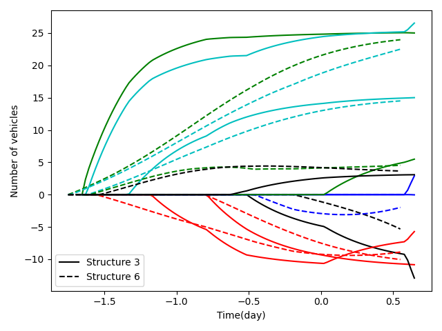

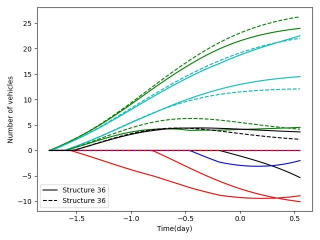
To facilitate later narrative, analysis and summary, travel patterns were grouped into four broad categories based on the combination of high and low indicators, which were identified as regular commuting patterns, special commuting patterns, short-time activity patterns and external errands patterns based on the qualitative nature of the indicators combined with manual judgement, and the qualitative characteristics and values of the indicators for the broad categories are shown in Table 1. Table 2 shows the results of the travel mode classification.
| Category | Difference in percentage of working days and rest days | Ratio of vehicles from other places | Peak travel ratio | Travel days | Entropy |
| Normal commuting mode | High (+19%) | Low (20%) | High (88%) | High (22%) | High (0.82%) |
| Special commuting mode | Medium (1) | Low (24%) | High (77%) | High (22%) | High (0.74%) |
| Short time activity mode | Low (- 9%) | High (29%) | Low (54%) | Low (15%) | Low (0.40%) |
| External service mode | Low (- 6%) | High (31%) | Low (51%) | Low (14%) | High (0.85%) |
| Category | Proportion% | Travel mode | |||
|---|---|---|---|---|---|
| Normal commuting mode | 43.3 | 3-1,3-2,6-4,17-2,36-1,36-2,38-2,38-4,63-2,63-5 | |||
| Special commuting mode | 1.6 | 11-1,11-2,11-3,17-4,38-1 | |||
| Short time activity mode | 29.0 | 3-3,3-4,17-1,36-3,36-4,36-5,38-3,63-1,63-3,63-4 | |||
| External service mode | 26.5 | 6-1,6-2,6-3,17-3,38-5 |
The vehicle behavior of the regular commuting pattern follows a work rhythm, with a high number of travel days and a significantly lower share of rest days than weekdays. This mode stays in one location for long periods of time during the day and participates in the morning and evening peaks, hence the high entropy and peak travel comparisons. The special commuting pattern is the rarest; this pattern has some of the commuting characteristics, with high entropy, days of travel and proportion of local vehicles, but does not follow the normal morning and evening commuting behavior, occasionally travelling during the midday and late night hours, with little difference between rest days and weekdays, and not necessarily returning to the residence at night. The short-time activity pattern is for non-work purposes, with a significantly higher proportion of rest days than weekdays, with trips generally staggered to peak periods, stopping at one or more locations, but with shorter periods of time and lower entropy per activity. The out-of-town errand mode shares similarities with the behavior of the short-time activity mode, also often travelling on rest days and during peak hours, differing in the number of stopping locations, the length of time and the high entropy, with the smallest proportion of local vehicles and the fewest days of travel, and with the first and last positions of \(1 d\) often differing. This is the pattern of people from outside the Xiao Shan District who travel to Xiao Shan on business or to visit friends and relatives and leave on the same day or stay in a hotel; foreign tourists who leave their residence during the day to visit the attractions and change their accommodation or leave Xiao Shan in the evening are also classified in this pattern.
This paper uses the results of the land use characteristics analysis to further analyze the travel behavior, purpose and nature of typical travel patterns by plotting the percentage change of land use characteristic categories at the stopping points based on the 24 h stopping locations of vehicles for each mode.
Typical of the regular commuting pattern is mode 3-1: from location 1 to location 2 at 7:00-8:00 and back at 17:00-18:00, belonging to the “9 to 5” commuters. According to Figure 12, the proportion of land use type C3 increases by more than 40% after Mode 3-1 switches from Location 1 to Location 2. These nodes have prominent business office attributes, in line with the commuting characteristics of corporate employees, while the proportion of C1 and C2 nodes with residential attributes decreases during this period. Pattern 36-1 also has commuting characteristics, but instead of returning directly to location 1 after work at location 2, it heads to location 3 for activities before returning home, possibly corresponding to a pattern of after-work dining and entertainment activities. This hypothesis can be corroborated with the land use distribution. During the Location 3 stay phase from 17:00-21:00, the proportion of nodes in the C3 category with office attributes decreases and the proportion of nodes in the C2 category, which has strong shopping consumption and entertainment characteristics, begins to increase, and the proportion of C1 nodes in the residential category returns to its initial level after the activity ends at 21:00.
The special commuting mode can be subdivided into two scenarios. The first special commuting pattern still travels during the morning peak hours but still works at night and does not return to their residence, as in pattern 11-1. This pattern travels from location 1 to location 2 in the morning peak, returns to location 1 for a short break between midday and early evening, and travels again to location 2 at night. location 1 has a strong residential class attribute, while location 2 has a high proportion of C3 company business and C4 public service nodes staying during its stay, and this segment of traveler work intensity is likely to be higher. The second pattern 17-4, shown in Figure 13, has a brief activity at location 2 at irregular times during the day, after which they return to their residence at location 1 and uniformly travel to location 3 after about 18:00 until day 2, and the proportion of nodes in the C3 and C4 categories both increase significantly, while the proportion of nodes in the C1 residential attribute decreases. This pattern may reflect the commuting patterns of night-time workers in consumer entertainment venues or night shift workers in public units such as hospitals [26].
In this paper, on the basis of reviewing a large amount of literature and information about the path planning and motion control of driverless vehicles, we summarize the current situation of the research on the path planning and motion control of driverless vehicles, focusing on the path planning of driverless vehicles and obstacle avoidance path tracking control to carry out relevant algorithms, mainly for solving the path re-planning of driverless vehicles in the environment with obstacles and the path tracking of driverless vehicles in 2 problems of path planning after obstacle avoidance path planning are proposed, and a driving trajectory planning method based on spatio-temporal analysis is proposed to project the perception results onto the 3D spatio-temporal navigation map. Through simulation verification, the whole process of the proposed trajectory planning method takes 51.27ms on average, and by adjusting the search conditions of the A* algorithm, the search speed is increased by 27.86% compared with the traditional algorithm, which improves the overall planning efficiency. The actual feeling and data results of the real vehicle experiment show its good tracking effect, which verifies the effectiveness and practicality of the algorithm proposed in this paper.
The author reviewed the results, approved the final version of the manuscript and agreed to publish it.
The experimental data used to support the findings of this study are available from the author upon request.
The author declared that they have no conflicts of interest regarding this work.