
With the development of the global economy, more and more tunnels are being built in different regions and the number of problems encountered is bound to increase [1,2]. Scholars have conducted numerous studies on the stability of tunnel envelopes. [3-5] used numerical methods to carry out studies on the influence of envelope stability under different ground stress releases and concluded that the larger the ground stress release, the smaller the load borne by the anchors and the wider the development of the plastic zone of the envelope [6]. The strain measurement technique was also used to measure the strain values at key parts of the tunnel and to analyse the stress variation law of the surrounding rock body [7-10]. The equivalent elastic modulus and equivalent lateral pressure coefficient of this type of surrounding rock after initial support were obtained by using the positive inverse analysis method.
Therefore, using existing research methods to analyse the influence of various factors on tunnel deformation and damage is of positive significance in improving the understanding of the deformation and damage mechanism of tunnel envelope pressure and the support mechanism of anchor rods, anchor cables and grouting. Due to the different degrees of non-homogeneity, anisotropy and development of joints in the surrounding rock, the stability of the tunnel envelope is closely related to the rock structure of the tunnel envelope, in addition to the tectonic and geological environment of the project area, the degree of burial and the mechanical parameters of the rock body [11]. In the process of tunnel rock stability analysis, the surrounding rock is not only the main body of the underground engineering body bearing structure, but also the main source of structural load, and the rock structure has an important influence on the characteristics of the secondary stress field distribution after excavation, the plastic zone of the surrounding rock, the support structure and the surrounding rock pressure, etc. Therefore, in the actual tunnel construction process, it is important to be able to accurately determine the structural characteristics of the surrounding rock and to classify them.
In the actual construction of tunnels, the ability to accurately determine the structural characteristics of the surrounding rock and classify them is a prerequisite and basis for the classification of the rock, the determination of the support structure parameters and the selection of the construction method [12]. In [13], by discussing the significance of rock structure and stability, structural stability and methods for finding ultimate loads, geotechnical material ontological relationships and geotechnical stability, and by combining the redundant force reinforcement method of finite element analysis, the energy criterion of non-linear stability analysis and the principle of structural stability potential energy, the method of finding ultimate loads, which is different from structural instability and material instability, is proposed and is particularly applicable to the field of complex structures, and in [14] took the physical and mechanical properties of rock structure surface and engineering geological rock group as the starting point, studied the special rock structure of tunnel envelope, and pointed out that the rock structure characteristics of tunnel envelope are mainly controlled by the tectonic extrusion fracture zone intersecting the tunnel axis at a small angle and the rock group with alternating hard and soft outputs, and concluded that the deformation and damage of tunnel envelope is mainly controlled by the rock structure. The results of this study are presented as a reference for the classification, design and construction of tunnel rock support structures in areas with complex engineering geological conditions; [15,16] by numerically simulating the structural surface network of the tunnel rock envelope and combining the structural characteristics of the rock mass, the ANSYS finite element analysis software is used to analyse and evaluate the displacement and stress fields in the initial state of the rock envelope, during excavation and after support in three cases, and thus this provides a strong basis for validating the support method for the tunnel rock [17,18].
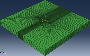
The analysis of tunnelling problems using finite element procedures requires a combination of calculation volume and accuracy. Theoretical and practical evidence shows that the stress distribution after excavation does not exceed 10 times the radius of the tunnel. Taking into account the specific engineering reality, the numerical model chosen for the calculation of the grade 3 surrounding rock is as follows: the lower part is taken to 80m below the bottom of the tunnel, the left and right side boundaries are taken to 60m outside the tunnel, the upper part is taken to 60m according to the actual burial depth of the tunnel, both sides are horizontally constrained, the bottom is vertically constrained, the analytical model is shown in Figure 1.
According to the engineering geomechanical properties of the rock mass, the Mohr-Coulomb strength damage criterion was adopted. The Mohr-Coulomb ideal elastoplastic model is used for the material model of the surrounding rock, solid units are used for the surrounding rock and initial support, and the initial ground stress of the surrounding rock is simulated by considering the self-weight stress to reach equilibrium, and the Mohr-Coulomb equal area circular yielding criterion is used for the calculation, which is expressed in Eq. (1).
\[\label{e1} F = \partial {I_1} + \sqrt {{J_2}} = k,\tag{1}\] where, \({I_1}\) and \({J_2}\) are the first invariant of the stress tensor and the second invariant of the stress deflection tensor, respectively.
\[\label{e2} {I_1} = {\sigma _1} + {\sigma _2} + {\sigma _3}.\tag{2}\]
\[\label{e3} {J_2} = \frac{1}{3}\left[ {\left( {{\sigma _1} – {\sigma _2}} \right) + \left( {{\sigma _2} – {\sigma _3}} \right) + \left( {{\sigma _3} – {\sigma _1}} \right)} \right].\tag{3}\] Here, \(\alpha\) and \(k\) are constants related to the angle of internal friction \(\phi\) and cohesion C of the geotechnical material, \(\alpha\), \(k\) satisfying the following relations, see Eq. (4) and Eq. (5).
\[\label{e4} \alpha = \frac{{2\sqrt 3 \sin \phi }}{{\sqrt {2\sqrt 3 \pi \left( {9 – {{\sin }^2}\phi } \right)} }},\tag{4}\]
\[\label{e5} k = \frac{{6\sqrt 3 C\sin \phi }}{{\sqrt {2\sqrt 3 \pi \left( {9 – {{\sin }^2}\phi } \right)} }}.\tag{5}\]
According to the engineering rock mechanical parameters obtained, the rock physical and mechanical parameters of the surrounding rock at different levels were obtained.
The specific parameters are shown in Table 1.
| Index/ Iithology | Severe(g/ \(c{m^3}\) ) | Compressive strength(Mpa) | Modulus of elasticity (GPa) | Cohesion (MPa) | Internal friction angle(°) | Poisson’s ratio |
|---|---|---|---|---|---|---|
| Granite | 2.6 | 65.1 | 50.2 | 25.3 | 40.5 | 0.22 |
| Granodiorite | 2.6 | 43.5 | 33.2 | 21.5 | 37.7 | 0.19 |
| limestone | 2.6 | 38.8 | 28.2 | 20.3 | 32.9 | 0.18 |
| Dolomite | 2.6 | 35 | 27.6 | 18.4 | 28.7 | 0.18 |
| Tuff | 2.5 | 32.9 | 32.9 | 18.5 | 26.3 | 0.17 |
The common methods of tunnel excavation are full section excavation, step excavation and step-by-step excavation. ABAQUS finite element software is very convenient for simulating the tunneling method of step-by-step construction excavation.
Earth stress balance
The initial stress is the initial stress in the tunnel rock, which largely influences the stability of the tunnel excavation. In tunnel excavation, the influence of the initial stress field needs to be considered first, and a ground stress balance must be established when the tunnel excavation is simulated numerically.
After the ground stress balance has been established, the tunnel excavation needs to be simulated in steps, the following is the excavation process from Grade II to Grade V surrounding rocks.
Class II Rock
The Class II rock is a hard rock with a simple rock cover and a relatively homogeneous rock quality, so the full section blasting method was used. The tunnel excavation sequence is shown in Figure 2.
Grade III Surrounding Rock
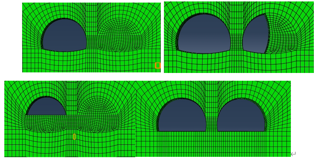
The rocks are slightly weathered, generally influenced by geological formations, with slightly developed joints and fissures and a blocky structure. The structural surface combination is basically stable. It is a basic stable rock, so the up and down step method is used. The specific sequence of tunnel excavation is shown in Figure 3.
Grade IV Surrounding Rocks
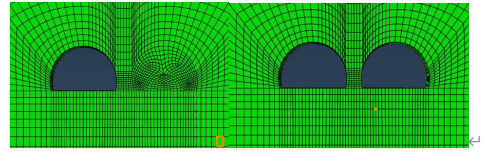
Grade IV surrounding rocks have more distribution of soft and weak structural surfaces, joint fissures are locally extremely developed, and the rocks have a rubble-like mosaic structure and a rubble-like crushed structure locally. This is a poorly stable rock, so a combination of up and down steps and positive sidewall guide pits is used. The tunnel excavation sequence is shown in Figure 4.
Grade V Rock
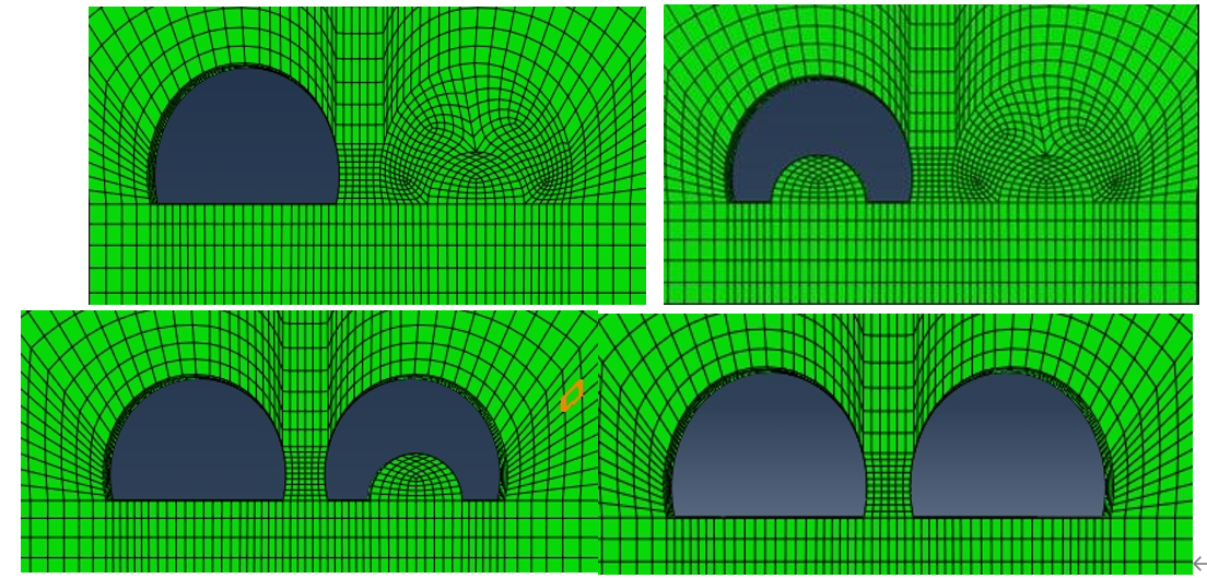
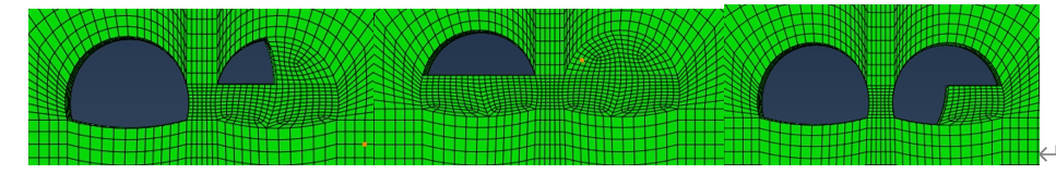
The Grade V surrounding rocks are strongly weathered or fully weathered rocks, severely affected by geological structures, with extremely developed joints and fissures, fault fracture zones greater than 2m in width and fissures filled with mud. The rock is extremely unstable, so a combination of up and down steps and positive sidewall guide pits is used. The tunnel excavation sequence is shown in Figure 5.
Maximum Principal Stresses
Figure 6 to 9 show the maximum principal stresses after excavation of the tunnels for Class II to Class V rock, respectively.
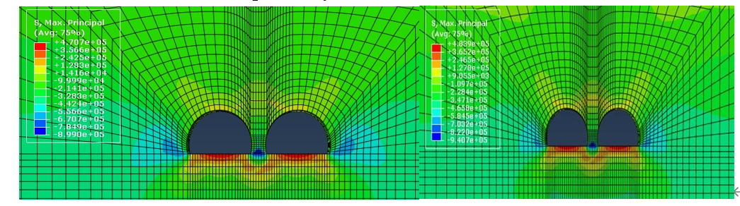
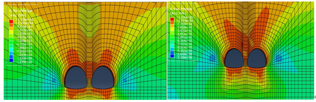
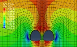
From Figure 6 to 9, the maximum principal stress distribution in the surrounding rock after tunnel excavation shows that the tensile stresses in the Class II surrounding rock are concentrated at the bottom and top of the tunnel, with a maximum tensile stress of 0.48MPa, located at the bottom of the tunnel; the tensile stresses in the Class III surrounding rock are concentrated at the bottom and top of the tunnel, with a maximum tensile stress of 0.45MPa, occurring at the bottom of the tunnel; the tensile stresses in the Class IV surrounding rock are concentrated at the bottom and top of the tunnel, with a maximum tensile stress of is 0.13MPa; tensile stresses are concentrated above the rock column in Class V, with a maximum tensile stress of 0.12MPa.
Minimum Principal Stresses
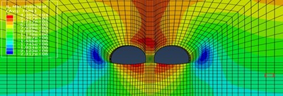
Figure 10 and 11 show the minimum principal stress distribution after excavation for small spaced tunnels from Class II to Class V surrounding rocks respectively.
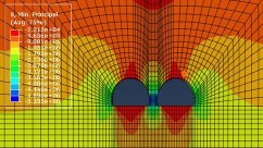
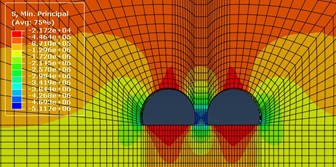
As can be seen from Figure 10 to 11, the minimum principal stresses in the surrounding rocks after tunnel excavation are concentrated in the rock column and on both sides of the tunnel, with a maximum compressive stress of 0.95 MPa at the bottom of the rock column. The maximum compressive stress is 0.52 MPa; the compressive stress concentration occurs near the rock column and the sides of the tunnel in Class V rock, with a maximum compressive stress of 0.33 MPa, occurring near the sides of the tunnel.
The problem of differentiating the quality of a rock mass by means of multiple indicators can be summarised as a comprehensive evaluation problem: let X be the evaluation object space, and its object \({x_i}\) (i= 1,2,… ,n) has m evaluated indicators \({I_j}\) (j= 1,2,… ,m). For each indicator \({I_j}\) measurement \({t_j}\) of \({x_i}\) , there are p evaluation levels \({C_k}\) (k= 1,2,… ,p), so that the level of \({t_j}\) can be determined and the \({x_i}\) can be evaluated together to determine its level.
The attribute identification model for comprehensive evaluation of rock quality classification consists of three aspects: single-indicator attribute measurement; multi-indicator integrated attribute measurement; attribute identification.
The size of the evaluated object \({x_i}\) with level \({C_k}\) is represented by the attribute measure \({\mu _{xk}} = {\mu _{{x_i}}} \in {C_k}\), and the size of the jth indicator value \({t_j}\) of \({x_i}\) with level \({C_k}\) is represented by the attribute measure \({\mu _{xk}} = {\mu _{{t_j}}} \in {C_k}\). \({\mu _{xk}} = {\mu _{{t_j}}} \in {C_k}\) is determined by establishing its attribute measure function to represent the change in the attribute measure \({\mu _{{t_j}}}\) due to a change in \({t_j}\).
Determine the single-indicator attribute measure function \({\mu _{xk}}\left( t \right)\) as follows:
\[\label{e6} \mu_{x k}(t)=\left\{\begin{array}{cc} 1 & t<a_{j 1}-d_j, \\ \frac{a_{j 1}+d_j-t}{2 d_j} & a_{j 1}-d_j \leq t \leq a_{j 1}+d_j, \\ 0 & a_{j 1}+d_j<t, \end{array}\right.\tag{6}\] where, \(j= 1,2,… ,m; k= 2,3,… ,p- 1.\)
Single indicator attribute measures are weighted and summed to obtain a composite attribute measure \({u_{xk}}\):
\[\label{e7} {u_{xk}} = \sum\limits_{j = 1}^m {{\omega _k}} k,\tag{7}\] where \({\omega _j}\) is the weight of the jth indicator \({I_j}\), satisfying:
\[\label{e8} {\omega _j} \geqslant 0,\quad \sum\limits_{j = 1}^m {{\omega _j}} = 1.\tag{8}\]
Confidence criterion: Let the evaluation set ( \(C_1, C_2, \cdots, C_K\)) be an ordered set and satisfy \(C_1>C_2>\cdots>C_K\), \(\lambda\) is the confidence level, which can be 0.5\(<\) \(\lambda\) \(\leqslant\) 1. If
\[\label{e9} {k_0} = {\text{m in\{ }}k:\sum\limits_{1 \ne 1}^{\text{k}} {{\text{ }}{\mu _{{\text{xk}}}}} \geqslant \lambda 1 \leqslant k \leqslant p\} ,\tag{9}\] then \(x\) is considered to belong to class \(C{k_0}\).
There are m evaluation indicators, which may or may not have the same importance. In this paper, we use the similarity number to define the similarity weight to give an objective weight to the evaluation indicators [18], in order to avoid the subjective preference brought by the expert assignment. The method and steps are as follows:
Assume that the weight values of each evaluation index are equal:
\[\label{e10} {\omega _j} = 1/m,\tag{10}\]
\[\label{e11} {\mu _{ck}} = \frac{1}{m}\sum\limits_{j \ne k}^m {{\text{ }}{\mu _{jk}}{\text{ }}} ,\tag{11}\] where, \(i= 1,2,… ,n; j= 1,2,… ,m; k= 1,2,… ,p.\)
In order to verify the validity and feasibility of the property identification model, a comparative analysis was carried out with the evaluation example of reference [19], and the data are shown in Table 2. With reference to the relevant research results, the comprehensive evaluation indexes of rock quality classification were determined as rock quality index RQD (%), uniaxial compressive strength (in MPa), joint spacing (in m), friction coefficient of joint surface f, the amount of groundwater infiltration Q in L (min-10m)] or the unit water absorption rate Q (in Lu). For excavated tunnels, it is convenient to use the measured seepage volume “L min” per 10m section of tunnel as the Q value. However, the size of the hole has a great impact on the amount of groundwater seepage, and there are obvious differences in the amount of groundwater seepage in different seasons, so using this to measure the quality of the rock seems to be somewhat imprecise, and the standard is not uniform. In water conservancy and hydropower projects, the results of borehole exploration are often used to judge the quality of the rock, especially in riverbed dams where drilling is much easier than exploring holes, even in underground plants, water transfer tunnels, diversion caverns and flood relief caverns, etc. In the process of site selection, drilling is often done first and then digging [20]. Therefore, the “water absorption rate per unit Q(Lu)” commonly used in water conservancy and hydropower engineering borehole exploration is more widespread. 1Lu=1L (min-MPa-m) means that under the action of 1MPa water pressure, in 1min, each 1m long borehole is absorbed by the rock body of 1L (litre) of water. It has nothing to do with the diameter of the tunnel and is very little affected by the season, so it is reasonable to use it to measure the quality of the rock, and there is a more uniform standard. It is therefore recommended to promote the use of the unit of water absorption rate Lu; in tunnels that have been excavated, if there are no conditions to do borehole pressure tests, we have to use the approximate unit of groundwater seepage L (min-10m). There is currently no conversion between the two, but they are roughly equivalent in terms of magnitude when used to describe the quality of the rock mass, so it is worth borrowing them for the time being and using the same quantitative scale. With reference to domestic and international experience in evaluating rock quality, rock stability is divided into five categories: Class I is stable, Class II is basically stable, Class III is poorly stable, Class IV is unstable, and Class V is extremely unstable. The relationships between the rock quality classes and the evaluation indicators are shown in Table 3.
| Sample number | RQD/% | \({R_c}\) /Mpa | \({J_1}\) /m | f | Q/Lu |
|---|---|---|---|---|---|
| A | 86 | 96.44 | 2.12 | 0.97 | 12 |
| B | 65 | 76.54 | 0.33 | 0.65 | 11 |
| C | 83 | 112.15 | 1.8 | 0.7 | 10 |
| D | 40 | 57.19 | 0.25 | 0.45 | 12 |
| E | 78 | 108.63 | 1.76 | 0.67 | 5 |
| Sample number | RQD/% | \({R_c}\) /Mpa | \({J_1}\) /m | f | Q/Lu |
|---|---|---|---|---|---|
| Sample number | Stable | Basically stable | Poor stability | Instable | Extremely unstable |
| RQD/% | 100-90 | 90-75 | 75-50 | 50-25 | \(<\)25 |
| \({R_c}\) /Mpa | 300-200 | 200-100 | 100-50 | 50-25 | \(<\)25 |
| \({J_1}\) /m | 5-3 | 3-1 | 1-0.3 | 0.3-0.05 | \(<\)0.05 |
| f | 12-0.8 | 0.8-0.6 | 0.6-0.4 | 0.4-0.2 | \(<\)0.2 |
| Q/Lu | 0-5 | 5-10 | 10-25 | 25-125 | 125-300 |
In step 1, we calculate the single indicator attribute measure. Based on the sample data in Table 2, the single-indicator attribute measures were calculated according to the single-indicator attribute measure function given in Table 4. According to Eq. (11), at this point \({\mu _{ck}} = \frac{1}{5}\sum\limits_{j \ne k}^m {{\text{ }}{\mu _{jk}}{\text{ }}}\), the attribute measure matrix \({\mu _{5 \times 5}}\) was obtained as:
\[\label{e12} \mu_{5 \times 5}=\left[\begin{array}{cccccccc} 0 & 204 & 0 & 488 & 0 & 308 & 0 & 0 \\ 0 & 0 & 243 & 0 & 757 & 0 & 0 & 0 \\ 0 & 073 & 0 & 823 & 0 & 104 & 0 & 0 \\ 0 & 0 & 020 & 0 & 493 & 0 & 487 & 0 \\ 0 & 107 & 0 & 732 & 0 & 161 & 0 & 0 \end{array}\right]\tag{12}\]
In the second step, the weights of each indicator \({I_j}\) were determined \({\omega _j}\) . According to Eq. (11) and Eq. (12), we get: similarity coefficient \({r_j}\) = (0.327,0.373,0.488,0.360,0.326), similarity weight \({\omega _j}\) = (0.174,0.199,0.260,0.192,0.174).
Finally in step 3, we Calculate the composite attribute measure and attribute identification. The composite attribute measure is calculated according to Eq. (11) \({\mu _{xk}}\) and formed into a composite attribute measure matrix \({\mu _{5 \times 5}}\).
\[\label{e13} \mu_{5 \times 5}=\left[\begin{array}{cccccccc} 0 & 185 & 0 & 530 & 0 & 284 & 0 & 0 \\ 0 & 0 & 225 & 0 & 775 & 0 & 0 & \\ 0 & 064 & 0 & 845 & 0 & 091 & 0 & 0 \\ 0 & 0 & 017 & 0 & 463 & 0 & 520 & 0 \\ 0 & 093 & 0 & 717 & 0 & 190 & 0 & 0 \end{array}\right]\tag{13}\]
Taking \(\lambda\)= 0.6, attribute identification was performed according to Eq. (13), and the comprehensive evaluation results of each sample were obtained.
The six factors affecting the amount of horizontal convergence and the amount of horizontal convergence were subjected to ANOVA and the results were calculated as shown in Table 4.
| Factor | Sum of squares of variance | Freedom | Mean square | F value | P |
|---|---|---|---|---|---|
| Correction model | 1832.454 | 12 | 152.704 | 35.348 | 0 |
| Modulus of elasticity | 521.092 | 2 | 260.546 | 60.311 | 0 |
| Poisson’s ratio | 59.043 | 0 | 29.521 | 6.834 | 0.037 |
| Internal friction angle | 480.403 | 2 | 345.720 | 80.027 | 0 |
| Cohesion | 691.144 | 2 | 345.720 | 80.027 | 0 |
| Tensile strength | 74.436 | 2 | 37.218 | 8.615 | 0.024 |
| Density | 60.4 | 2 | 3.02 | 0.699 | 0.54 |
| Error | 21.6 | 5 | 4.32 | – | – |
| Total | 20878.906 | 18 | – | – | – |
As can be seen in Table 4, the F-statistic for the horizontal convergence model is 35.348 with a probability level P-value of 0.000, which shows that this ANOVA is highly significant. The different magnitudes of the F-values for each factor indicate that each factor has a different degree of influence on the level of convergence.
The six factors affecting the amount of sinking in the vault and the amount of sinking were subjected to ANOVA and the results were calculated as shown in Table 5.
| Factor | Sum of squares of variance | Freedom | Mean square | F value | P |
|---|---|---|---|---|---|
| Correction model | 5617.281 | 12 | 468.106 | 39.941 | 0.001 |
| Modulus of elasticity | 703.174 | 2 | 351.589 | 25.497 | 0.002 |
| Poisson’s ratio | 129.007 | 2 | 64.509 | 75.957 | 0.007 |
| Internal friction angle | 2444.642 | 2 | 1222.321 | 88.633 | 0.001 |
| Cohesion | 228.912 | 2 | 114.457 | 8.298 | 0.025 |
| Total | 9191.968 | 25 | – | – | – |
As can be seen from Table 5, the F-statistic for the model for the amount of vault subsidence is 39.941 with a probability level P-value of 0.001, which shows that this ANOVA is very significant. The different magnitudes of the F-values for each factor indicate that each factor has a different degree of influence on the amount of vault subsidence.
The six factors affecting the shaping zone factor and the shaping zone factor were subjected to ANOVA and the results were calculated as shown in Table 6.
| Factor | Sum of squares of variance | Freedom | Mean square | F value | P |
|---|---|---|---|---|---|
| Correction model | 30.457 | 12 | 2.521 | 16.524 | 0.002 |
| Modulus of elasticity | 0.627 | 2 | 0.314 | 2.027 | 0.233 |
| Poisson’s ratio | 14.58 | 2 | 7.286 | 47.821 | 0.001 |
| Internal friction angle | 12.974 | 2 | 6.458 | 42.567 | 0.001 |
| Cohesion | 1.547 | 2 | 0.774 | 5.064 | 0.059 |
| Tensile strength | 0.761 | 5 | 0.151 | – | – |
| Total | 60.946 | 25 | – | – | – |
As can be seen in Table 6, the F-statistic for the plastic zone factor model is 16.524 with a probability level of 0.003, which shows that this ANOVA is highly significant. As the magnitude of the F-value for each factor varies, it indicates that each factor has a different degree of influence on the plastic zone factor. The F-value of each factor was used to determine the magnitude of its influence.
In order to analyse the influence of each factor on the horizontal convergence, vault subsidence and plastic zone factor of the tunnel more intuitively, the statistical results in the ANOVA of the horizontal convergence, vault subsidence and plastic zone factor were used to plot the influence curves of each factor on the horizontal convergence, vault subsidence and plastic zone factor, respectively, using the level of each factor as the horizontal coordinate and the corresponding mean as the vertical coordinate, as shown in Figure 12.
As can be seen from Figure 12 and the above analysis, the modulus of elasticity, Poisson’s ratio, angle of internal friction, cohesion and tensile strength all have an influence on the horizontal convergence, vault subsidence and plastic zone factor of the tunnel, but to different degrees.
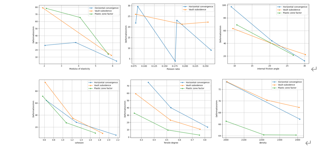
The changes in the horizontal convergence, vault subsidence and plastic zone factors of the tunnel envelope after changing any of the six factors are shown in Figure 13.
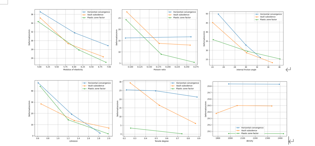
Figure 13 shows that when only the modulus of elasticity, angle of internal friction, cohesion and tensile strength are varied, the horizontal convergence, vault subsidence and plastic zone factor all decrease as the values of these four factors increase. The stability of the surrounding rock is the ability of the surrounding rock not to deform after excavation of an underground chamber such as a tunnel. Consideration of the stability of the tunnel envelope should take into account the amount of horizontal convergence, the amount of vault subsidence and the plastic zone factor after excavation of the tunnel.
The study adopted the Mohr-Coulomb strength damage criterion for assessing rock mass behavior during tunnel excavation. Engineering mechanics parameters were determined based on rock physical and mechanical properties, facilitating numerical simulation of excavation processes. Various excavation methods were employed according to rock stability classification, with stress field characteristics analyzed post-excavation. A property identification model was proposed for rock quality classification, integrating single and multi-indicator measures. An example assessment demonstrated the model’s application in evaluating rock stability.
This study received the following funding support: Suzhou University, Suzhou City, Anhui Province Project Fund Number: 2023BSK071.