
How to effectively combat crime, which affects the quality of life of citizens and the economic development of society, is one of the well-known challenges of social governance. There are two types of crimes that are more common, one is crimes against property security, such as theft, burglary and robbery. The other category is crimes against personal safety, such as homicide, assault and criminal damage [20,13,14].
When there is crime, naturally there is crime fighting. How to effectively combat crime and reduce the crime rate has always been the goal of the police and experts and scholars who have been working tirelessly. Dating back to the beginning of the 20th century, the focus of expert scholars on the study of criminal activities is the evolution of criminal behavior and the interrelationship between criminal activities and the social environment in which they are located [2,12]. The social network, community characteristics, and poverty index of a particular person were regarded as important influencing factors, and with the release of desensitized criminal records in some foreign cities in recent years, scholars have begun to use these data as the basis for macro research on criminal activities, in order to mine potential criminal patterns from a large amount of criminal data, and to make predictions about possible future criminal activities [15,19,5].
Increasingly mature data mining techniques have rapidly promoted the development of data-driven crime prediction research. Graph neural networks are often used to extract spatial features of crime data, and recurrent neural network family models and temporal convolutional networks are often used to extract temporal features of crime data [1,7,4]. These neural network models significantly improve the accuracy of crime prediction compared to traditional crime analysis methods. The process of digitization in modern cities generates a huge amount of data, which can reflect every aspect of citizens in their lives, and also provide data supplements for crime prediction research. Taking data such as bicycle rental and cab traffic as examples, they reflect the connection between different areas and can explain the diffusion pattern of criminal activities in time and space from the aspect of population flow [11,8,23,9].
More and more scholars have begun to introduce these urban data into the study of crime prediction, such as census data, cab flow data, point-of-interest data, and urban anomaly data. In general, criminal activities bring no small threat to the personal safety, property security and social stability of citizens, and the research on crime prediction techniques aiming at combating criminal activities has emerged [22,10]. Increasingly mature data mining technology and the massive urban data spawned by urbanization both promote the rapid development of crime prediction technology. The development of crime prediction technology on the one hand helps public security organs to perceive the changing trend of criminal activities in the coming period of time, and provides a data basis for the formulation of future anti-crime policies. On the other hand, its temporal and spatial prediction results can help police officers optimize patrol routes, enabling more reasonable deployment of limited police forces. The contemporary world’s eagerness for big data crime prediction technology is actually in response to the serious security anxiety and to gain a sense of security through the preemptive strike strategy of big data crime prediction technology [3,16,6].
In this paper, we study the trend of crime occurrence in a specific time and space, determine the research direction about crime prediction, refer to the application examples of crime prediction model in criminal justice, propose the graph embedding model derived from graph neural network, establish the spatial channel attention mechanism, and obtain the important space and channel from the spatial convolution module, so as to improve the performance of the model. Generate the set of crime matrices, use the new loss function as the objective function for model training, combine with GRU algorithm to compose GAERNN model, and propose its predictive performance evaluation index. Through the study of existing literature, the correlation between spatio-temporal environmental elements and crime occurrence is proposed, and the relative spatio-temporal neural network model is added on the basis of the GAERNN model to complete the construction of the spatial prediction model of crime based on spatio-temporal environmental elements.
Research on crime prediction ranges from studies on the prediction of certain types of crime in a given place or period to studies on the development of predictive models.
Research on crime prediction within a specific time period. Based on the trends in crime occurrence in China in 2022, it is predicted that the number of crimes will increase in 2023, and that traditional street burglary and fraud crimes may rebound, while emphasis should be placed on preventing crimes of extreme personal violence and new types of crime triggered by new technological changes on the Internet.The trend of a continuous decrease in the mortality rate of intentional injuries in China from 2008 to 2020 predicts that the mortality rate of intentional injuries among Chinese residents will continue to decrease in the next The mortality rate of intentional injuries among Chinese residents will continue to decline over the next five years.
An important capability of data mining is the prediction of behavior [17]. In contrast to recording and recognizing ongoing criminal activity, an algorithm has been developed at the University of Houston with funding from the National Institute of Justice. It allows for continuous monitoring, assessing behavior and predicting sudden suspicious events and criminal behavior through a network of cameras. This work also works to identify and reacquire persons of interest across multiple cameras and images through clothing, bone structure, movement and orientation prediction.
Graph autoencoder (GAE) is a graph embedding model derived from neural networks, which uses a GCN encoder and inner product decoder to obtain an optimal representation by graph data reconstruction [18]. Due to its concise coding and decoding structure and efficient coding capability, GAE has been widely used in face recognition, biomedicine, and other fields.
The encoder is implemented using a two-layer GCN to aggregate the neighborhood node features to obtain the optimal representation of the nodes, and the process is represented as follows: \[\label{GrindEQ__1_} Z=GCN(X,A) . \tag{1}\]
Given the node feature matrix \(X\in R^{N} \times P\) and the adjacency matrix \(A\in R^{N\times N}\), which are input to the GCN function, the output \(Z\in R^{N\times F}\), where \(z_{i} {\rm }R^{F}\) is the representation vector of the node and \(F\) is the node representation dimension, the GCN is computed as: \[\label{GrindEQ__2_} GCN(X,A)=\tilde{A}ReLU(\tilde{A}XW_{0} )W_{1} , \tag{2}\] where \(\tilde{A}=D^{-\frac{1}{2} } AD^{-\frac{1}{2} }\), \(D\) are the degree matrices of the nodes, \(W_{0}\) and \(W_{1}\) are the parameters to be learned.
The decoder consists of two parts: neighbor matrix decoding and node feature decoding, so the loss function of GAE consists of the loss function corresponding to the reconstructed neighbor matrix and reconstructed node features, respectively. Among them, the adjacency matrix determines the structure of the graph, and the more similar the adjacency matrix reconstructed by the nodes’ low-dimensional representations is to the original matrix, it means that the low-dimensional representations of the nodes are more consistent with the structure of the graph, which in turn uses the cross-entropy function to measure the difference between the original adjacency matrix and the reconstructed adjacency matrix. The node feature matrices determine the properties of the graph, the more similar the node feature matrices reconstructed by the low-dimensional representations of the nodes are to the original matrices, the more the low-dimensional representations of the nodes conform to the properties of the graph, which in turn uses the root-mean-square error to measure the difference between the original node feature matrices and the reconstructed node feature matrices. The smaller the difference between the reconstructed matrix and the original losers, it means that the optimal representation of the node obtained \(z\) is able to retain more spatial information.The formula for the GAE loss function is as follows: \[\label{GrindEQ__3_} L_{1} =-\frac{1}{N} \sum _{i=1}^{N}y_{i} \log \left(1-y_{i} \right)+\hat{y}_{i} \log \left(1-\hat{y}_{i} \right) , \tag{3}\] \[\label{GrindEQ__4_} L_{2} =RMSE(X,\hat{X}) , \tag{4}\] \[\label{GrindEQ__5_} L=L_{1} +L_{2} , \tag{5}\] where \(y\) represents an element (0 or 1) in the adjacency matrix \(A\), \(\hat{y}\) represents the value (between 0 and 1) of the corresponding element in the reconstruction matrix \(\hat{A}\), \(x\) is the original node feature matrix, \(\hat{x}\) is the reconstructed node feature matrix, RMSE represents the calculation of the root mean square error, \(L_{1}\) is the loss function of the reconstructed adjacency matrix, \(L_{2}\) is the loss function of the reconstructed node features, and \(L\) is the total loss function.
The spatial channel attention mechanism enables the model to adaptively focus on important spaces and channels in the features acquired from the spatial convolution module, thus improving the performance of the model.
Channel attention computes the global average pooling and global maximum pooling of the input features by calculating the global average pooling and the global maximum pooling, joining the two and calculating the weights through the fully connected layer. And then these weights are applied to the channel dimensions of the input features. This weighting helps the model to focus on more meaningful feature channels in a particular task. The formula is as follows: \[\label{GrindEQ__6_} M_{c} (F)=\sigma (MLP(Avg\;Pool(F))+MLP(Max\;Pool(F))) , \tag{6}\] where, \(M_{c} (F)\) is the channel attention module, \(\sigma\) is the sigmoid function, MLP is the multilayer perceptron, and Avg Pool \((F)\) and Max Pool \((F)\) denote average and maximum pooling respectively.
The spatial attention calculates the weights by computing the average and maximum values of the input features along the channel dimension, joining the two and calculating the weights through a convolutional layer. And then these weights are applied to the spatial dimensions of the input features. This weighting helps the model to focus on more meaningful spatial regions in a particular task. The formula is given below: \[\label{GrindEQ__7_} M_{s} (F')=\sigma (f([Avg\;Pool(F'),\;Max\;Pool(F')])) , \tag{7}\] where, \(M_{s} (F^{{'} } )\) is the spatial attention module, \(\sigma\) is the sigmoid function, \(f\) is the convolution operation, and Avg Pool \((F^{{'} } )\) and Max Pool \((F^{{'} } )\) denote average and maximum pooling, respectively.
In order to map the time window dimension from \(\alpha \times NF\) to size \(\beta \times NK\), the output \(Y\in R^{a\times NF}\) of the time-aware self-attention module is therefore plugged into a two-dimensional convolutional network, Conv2d, for the purpose of dimension transformation. As a result, a collection of crime matrices \(\widehat{{\rm {\mathcal X}}}\in R^{\beta \times NK}\) (including the time, place and category of the crime) with a future time window of \(\beta\) can be generated: \[\label{GrindEQ__8_} \widehat{{\rm {\mathcal X}}}=\{ \hat{X}_{1} ,\hat{X}_{2} ,\cdots ,\hat{X}_{\beta } \} ={\rm Conv2d}(Y)\in R^{\beta \times NK} . \tag{8}\]
In order to stabilize the model training and accelerate the model convergence speed, the binary cross entropy (BCE) li IDice Loss is fused in the downstream binary classification task by using the auto loss weight-topping equilibrium (AWL) mechanism to form a new loss as an objective function for model training. The output of the model is 0 indicating that the crime does not occur and vice versa. The objective function consists of two parts [21]: \[\label{GrindEQ__9_} {\rm {\mathcal L}}(\widehat{{\rm {\mathcal X}}},\Theta )=AWL({\rm {\mathcal L}}_{BCE} (\widehat{{\rm {\mathcal X}}},\Theta ),{\rm {\mathcal L}}_{DL} (\widehat{{\rm {\mathcal X}}},\Theta )) \tag{9}\]
Where, BCE is a binary cross entropy calculation, formalized as follows: \[\label{GrindEQ__10_} {\rm {\mathcal L}}_{BCE} (\widehat{{\rm {\mathcal X}}},\Theta )=-\sum _{\xi }^{\beta }X_{t+\xi } log(\hat{X}_{t+\xi } )+(1-X_{t+\xi } )(1-log(\hat{X}_{t+\xi } )) . \tag{10}\]
DL is DiceLoss computation, a loss function for image segmentation and semantic segmentation tasks, which mainly calculates the loss by comparing the overlap region between the model output and the real label. The formal expression is as follows: \[\label{GrindEQ__11_} {\rm {\mathcal L}}_{DL} (\widehat{{\rm {\mathcal X}}},\Theta )=\sum _{\xi }^{\beta }\left(1-\frac{2\sum X_{t+\xi } \hat{X}_{t+\xi } }{\sum X_{t+\xi } +\sum \hat{X}_{t+\xi } } \right) . \tag{11}\]
In this paper, we propose a graph self-coding recurrent neural network (GAERNN) model based on GAE and GRU. Since the essence of the crime prediction problem is to learn a function \(f\) that predicts the number of crimes in each neighborhood in the future \(m\) time period based on the given multidimensional feature data \(X=(x_{1} ,x_{2} ,\cdots ,x_{i} )\) and graph data \(G\). \(Y=(\begin{array}{c} {y_{t+1} ,y_{t+2} ,\cdots ,y_{t+m} } \end{array})\) Therefore, the spatio-temporal prediction model of burglary crime in this paper can be represented as follows: \[\label{GrindEQ__12_} \left[\begin{array}{c} {y_{t+1} ,y_{t+2} ,\cdots ,y_{t+m} } \end{array}\right]=f\left(\begin{array}{c} {\left[\begin{array}{c} {x_{1} ,x_{2} ,\cdots ,x_{t} } \end{array}\right],G} \end{array}\right) . \tag{12}\]
The model first uses GAE to obtain the node optimal representation \(Z\in R^{N\times F}\) and inputs it into the downstream GRU to obtain temporal features, and finally the crime spatio-temporal prediction sequence is processed by the fully connected layer.
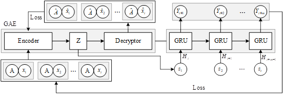
The structure of the GAERNN model is shown in Figure 1. Firstly, the neighbor matrix \(A\) and node feature matrix \(X=(x_{1} ,x_{2} ,\cdots ,x_{i} )\) with topological relations are sequentially input into GAE, the input data are encoded by encoder, and the reconstructed neighbor matrix \(\hat{A}\) and reconstructed node feature matrix \(\hat{X}\) are obtained using the decoder, and at the same time, the parameters of the model are optimized, so that the reconstruction result is as similar as possible to the original inputs, and thus the node optimal representation is obtained \(Z=(z_{1} ,z_{2} ,\cdots ,z_{i} )\) Then, the spatio-temporal information with temporal sequence data with spatial information is input to GRU, and through the information transfer between the units, the temporal dependence of the crime cases is further processed to obtain the spatio-temporal prediction feature sequence \(Y=(\begin{array}{c} {y_{t+1} ,y_{t+2} ,\cdots ,y_{t+m} } \end{array})\) through the fully connected layer at last.
During the training process, the goal is to minimize the error between the actual crime values and the predicted crime values as much as possible. Therefore, the loss function formula of GAERNN model is as follows: \[\label{GrindEQ__13_} Loss=MSE(C_{ture} ,C_{pre} )+L , \tag{13}\] where: \(C_{ture}\) represents the actual crime value and \(C_{pre}\) represents the predicted crime value.
Since the number of crimes in a given region may be zero and rarely extreme, three metrics, Root Mean Square Error (RMSE), Mean Square Error (MSE) and Mean Absolute Percentage Error (MAPE), are selected in this paper to measure the predictive performance of different crime prediction models. Among them, RMSE and MSE are used to assess the overall absolute prediction accuracy, the smaller the values of RMSE and MSE, the closer the predicted value is to the true value, and the better the model’s performance is.MAPE is used to measure the relative error, and a MAPE of 0% indicates a perfect model, while a MAPE of more than 100% indicates a poor quality model. The formulas for the above 3 indicators are as follows: \[\label{GrindEQ__14_} RMSE=\sqrt{\frac{1}{n} \sum _{i=1}^{n}\left(y_{i} -\hat{y}_{i} \right)^{2} } , \tag{14}\] \[\label{GrindEQ__15_} MSE=\frac{1}{n} \sum _{i=1}^{n}\left(y_{i} -\hat{y}_{i} \right)^{2} , \tag{15}\] \[\label{GrindEQ__16_} MAPE=\frac{1}{n} \sum _{i=1}^{n}\left|\frac{y_{i} -\hat{y}_{i} }{y_{i} } \right| \times 100\% , \tag{16}\] where: \(n\) represents the number of samples, \(\hat{y}_{i}\) represents the predicted value, and \(y_{i}\) represents the true value.
It has been shown that there is a correlation between spatio-temporal environmental elements and the occurrence of crime, i.e., there is a correlation between the local spatio-temporal environmental features where the crime is located and the occurrence of criminal activity. This type of model defines the local spatio-temporal environment feature as a raster area (or contains its neighborhood) divided according to certain experience, processes the currently processed local spatio-temporal environment feature (which may also contain case information) into a feature vector as an input in a certain way, and then calculates the correlation between this feature vector and the local spatio-temporal case information.
Risk terrain modeling
Risk terrain modeling is a typical multi-raster layer analysis model (RTM).1) List the variables related to the current crime to be predicted based on the available data and plot these variables on different layers, then project the existing spatio-temporal coordinates of the crime according to the equal-length time slices onto the layers to form multiple sub-risk layers.2) Perform regression analysis on the multiple sub-risk layers, and use the generalized linear model to determine the functional relationship between each factor and criminal activity, as well as the spatial and temporal transfer law of criminal activity. 3) Calculate the value of crime risk through the functional relationship derived from step 2, and use it as the basis for spatio-temporal prediction of crime, i.e., the spatio-temporal distribution of crime can be predicted in the future.
The risk map of the type of criminal activity can be generated by the above 3 steps. Risk terrain modeling quantifies the risk value of each element by analyzing the relationship between historical criminal activities and elements of the surrounding environment (POIs such as bars, hotels, Internet cafes, and also travel elements such as bus stops and subway stations), and the layers formed by using a variety of data sources are superimposed to form the final spatio-temporal prediction effect.
Bayesian prediction modeling
Some researchers believe that the occurrence of criminal activity conforms to a binomial statistical distribution (generally Poisson distribution), i.e.: \[\label{GrindEQ__17_} Y_{it} \sim Binomial(n_{it} ,p_{it} ) , \tag{17}\] where: \(Y_{i}\) represents the number of crimes, \(n_{i}\) represents the potential crime targets, \(p_{ii}\) represents the crime rate, \(i\) is the spatial area number, and \(t\) is the temporal order number. The logical functional form of criminal activity can generally be expressed as follows: \[\label{GrindEQ__18_} \log it(p_{it} )=\alpha +A_{i} +B_{t} +C_{it} , \tag{18}\] where: \(\alpha\) is the logarithm of the average relative risk of criminal activity, \(A_{i}\) is the spatial effect of criminal activity, including spatial non-structural effects \(U(i)\) and structural effects \(S(i)\), the former reflecting spatial heterogeneity, the latter reflecting spatial correlation, and the a priori distribution of the spatial structural effects mostly expressed as conditional autoregression or simultaneous autoregression. The a priori distribution of the spatial structural effect is mostly conditional autoregressive or simultaneous autoregressive. \(B_{i}\) represents the time effect, whose a priori distribution is generally expressed as a first-order autoregressive, and \(C_{ii}\) represents the space-time interaction effect. In order to synthesize data from multiple sources to improve the prediction accuracy of the model, the generic expression for the logistic function of criminal activity is as follows: \[\label{GrindEQ__19_} \log it(p_{it} )=\alpha +\beta X_{it} +A_{i} +B_{t} +C_{it} , \tag{19}\] where: \(\beta X_{n}\) is other spatio-temporal variables with potential impacts, such as site type, POI information, and community information. The model is operated by the MCMC algorithm, and the common comparison indexes are Akaike Information Criterion (AIC), Bayesian Information Criterion (BIC), and Departure Information Criterion (DIC).
The difference between the neural network model with relative time added and the traditional neural network structure is that the input of the input layer contains relative time information, and the neural network model structure with relative time added. Where the input to the model input layer is a spatio-temporal sequence of crimes with a time delay of \(n\), which can be represented as \(Z_{i} (t-1),Z_{i} (t-2),\cdots ,Z_{i} (t-n)\). The predicted value \(\tilde{Z}_{s} (t)\) of the number of crimes for region \(s\) in time period \(t\) can be represented as shown in equation (20): \[\label{GrindEQ__20_} \tilde{Z}_{s} (t)=F\left(\sum _{k=1}^{n}\beta _{sk} f(z_{s} (t-k),t_{k} )+\beta _{k} \right) . \tag{20}\]
In the above equation, \(t_{k}\) denotes the relative time, \(\beta _{sk}\) denotes the weights of the neuron nodes in the input layer and the neuron nodes in the hidden layer, \(\beta _{k}\) denotes the constant bias of the neurons, \(n\) denotes the maximum time delay order of the model, \(f\) denotes the nonlinear activation function of the hidden layer that contains the sigmoid function, and the output function \(F\) denotes the linear function.
After analyzing the relationships in each pattern set, networked modeling was performed using an improved graph self-coding recurrent neural network. In the modeling process, the topology of the community network was represented using a traditional adjacency matrix (i.e., an undirected binary adjacency matrix) with a view to identifying spatial dependencies of community crimes. In order to capture the serial correlation at each sub-frequency, a modified graph self-coding recurrent neural network was used to model the dynamic time-series trends of the modal sets of the community network. Table 1 shows the prediction performance evaluation of 78 communities in each modal set and the average results of the prediction of all community crimes, where M1-M8 are the results of the hierarchical prediction evaluation of each modal set, and the GAERNN algorithm is the average evaluation of the prediction of the actual number of crimes in 78 communities, which is determined based on the summation of all the modal sets of the corresponding nodes. The \(R^{2}\) of the predictions for all modal sets except M8 reached 0.9 or more, and after summing all modalities by corresponding nodes, the \(R^{2}\) value was 0.795484, and the MAE, MSE, and RMSE were 0.035984, 0.001987, and 0.043985, respectively.
From Table 1, it can be seen that the predictive performance of the model gradually decreases as the frequency of the modal set increases, which suggests that the model is able to capture the spatio-temporal dependence of community crime at low and medium frequencies by hierarchically extracting the long-term trend and medium-term seasonality of each community node from the original graph structure data. However, the predictive performance of high-frequency components such as M8, which reflects the short-term stochasticity of community crime, decreases compared to the low- and medium-frequency sequences. Thus, while the graph self-coding recurrent neural network is able to capture the medium- and long-term aggregation and spillover effects of community crime, the serial correlation between high-frequency components is very weak for the community network, which means that short-term inter-community volatility cannot be explained by each other, leading to poor prediction of the high-frequency components.
| \(R^2 \) | \(MAE\) | \(MSE\) | \(RMSE\) | |
| M1 | 0.982563 | 0.001388 | 0.000005 | 0.001955 |
| M2 | 0.994587 | 0.000678 | 0.000002 | 0.000963 |
| M3 | 0.994863 | 0.001489 | 0.000001 | 0.001588 |
| M4 | 0.988745 | 0.001486 | 0.000004 | 0.002369 |
| M5 | 0.976935 | 0.002766 | 0.000009 | 0.002741 |
| M6 | 0.934887 | 0.003485 | 0.000024 | 0.004956 |
| M7 | 0.906447 | 0.004688 | 0.000059 | 0.006485 |
| M8 | 0.678566 | 0.006528 | 0.000096 | 0.009188 |
| GAERNN | 0.795484 | 0.035984 | 0.001987 | 0.043985 |
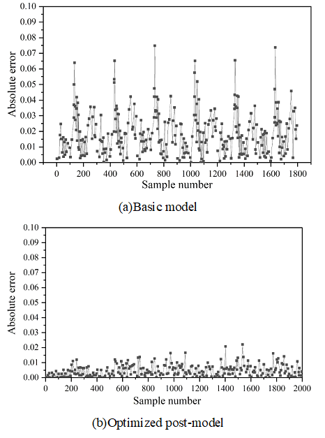
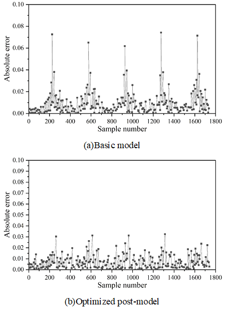
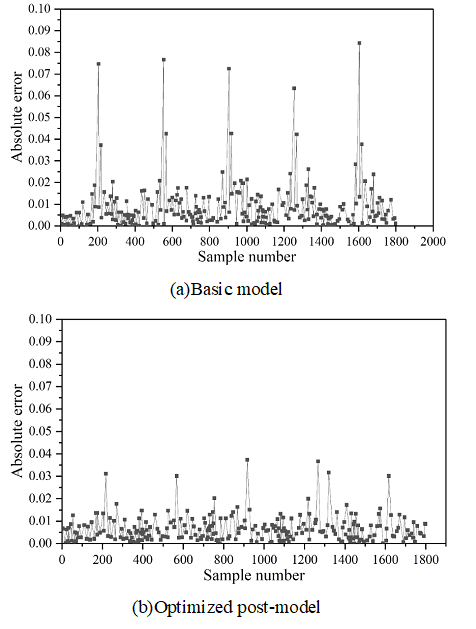
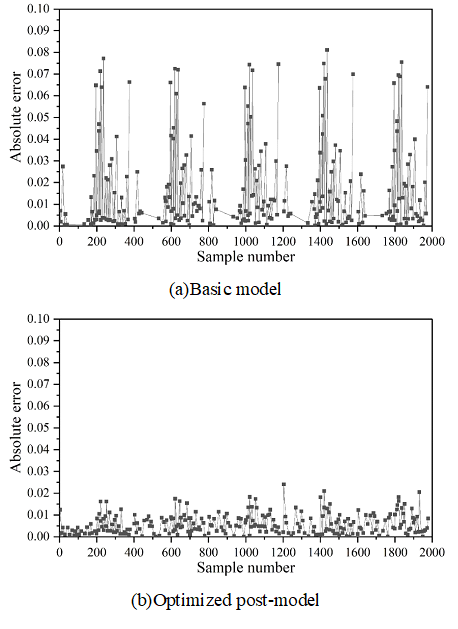
Figures 2- 5 show the comparison of absolute errors of quantity prediction for theft, assault, battery, and criminal damage, respectively, which can be more intuitively compared with the prediction effect of the prediction model after feature optimization and the base model under the same coordinate scale, which are represented by Figures (a) and (b), respectively.
As can be seen from the figure, except for the theft case, the prediction results after feature optimization in the other three types of cases have multiple error peaks, which is due to the special social situation when the case occurs or the abnormal performance of the perpetrator of the crime. The occurrence of crimes is affected by many factors, so the reasons for these peaks are complicated and it is difficult to predict their regularity accurately. However, it is obvious that the overall performance of the model after feature optimization has been improved to a greater extent, and the absolute error of prediction of the optimized model does not exceed 0.05, indicating that the optimization is able to better reflect the trend of the occurrence of crime in time and space.
The following is a comparison of all the experimental results in this section of the PEI index to analyze the two types of quantitative crime prediction algorithms on the prediction of burglary effect, in order to facilitate the expression of the first 0.5% of the crime risk, 1%, 5%, 10% of the crime risk level for the first four types of crime risk, respectively: very high risk, high risk, medium risk, and low risk. In this paper, the number of points of burglary cases in the next month accurately predicted by the geospatial space included in the four different crime risk levels were counted, and the PEI index and hit rate were calculated and counted, and six comparative experiments were conducted, and the results of the experiments are shown in Table 2 below.
The hit rates of the GAERNN algorithm are all higher or equal to the IsotDM algorithm, especially in the two crime risk levels of very high risk and high risk, the hit rates are significantly higher than those of the IsotDM method: for example, the average hit rate of the traditional IsotDM algorithm’s prediction in the very high risk level and the high risk level is only 7.3% and 14.58%, and the average PEI indexes are respectively 13.35 and 12.15, while the GAERNN algorithm achieves an average hit rate of 20.98% and 25.77%, with PEI metrics of 36.96 and 24.22, respectively. The improved predictive efficacy of the GAERNN algorithm relative to the IsotDM algorithm suggests that close to one-fifth of the next month’s burglaries will take place in the study area, which only represents 0.5% or 1% of the study area for this experiment. This means that nearly one-fifth of the burglary cases in the next month occur in the geographic space that only accounts for 0.5% or 1% of the study area, and if we focus on defending this area, we can get better crime prevention results, and also save a lot of human and financial resources for the public security department. In the two crime risk levels of medium-risk and low-risk, the gap in the prediction efficacy of the two types of prediction methods is gradually narrowing, and the hit rates of the IsotDM algorithm have achieved 25.63% and 32.47%, respectively. 32.47%, with PEI indicators of 5.44 and 3.46, respectively, while the GAERNN algorithm is 32.23% and 43.13%, with PEI indicators of 6.41 and 4.39, respectively.As the crime risk level decreases, the predictive efficacy of GAERNN algorithm is gradually approaching that of the IsotDM method, which is attributed to the fact that the theoretical basis of this paper is the same as that of the IsotDM method, and the same are based on the theory of proximity repetition, the difference is that the GAERNN algorithm introduces the environmental similarity of the geographic unit in which the case is located, which increases the dimensions of crime risk assessment.
The traditional IsotDM algorithm performs simple crime risk smoothing and diffusion for the crime risk value of each raster in the geospatial space to simulate the spatio-temporal process of crime risk described by the near-repeat theory, without considering the variability of the socio-environmental factors of the different geographic units in the geospatial space where the case itself is located, and ignoring the environmental attributes of the geospatial space where the burglary case is located itself. The algorithm in this paper makes up for the lack of expression of spatial differences in the traditional diffusion model based on the theory of proximity repetition by utilizing the diffusion coefficient function to describe the variability of environmental factors in different buildings in the study area, which in turn improves the efficacy of crime prediction based on the correlation that exists between the spatial differences of different environmental factors and the crime rate. The method in this paper shows obvious advantages over the traditional IsotDM algorithm in the crime prediction of the two crime risk levels of high risk and very high risk, so the advantage of the GAERNN algorithm over the traditional IsotDM algorithm is that it can utilize the crime risk hotspot area of a smaller area to predict more crime events, and the spatial resolution of the prediction result reaches the building level, which is This provides a strong support for the public security department to carry out targeted crime prevention work.
| / | Extremely high risk(0.5%) | High risk(1%) | |||
| Hit rate | PEI | Hit rate | PEI | ||
| January (45 cases) | IsotDM | 0.054 | 11.486 | 0.186 | 11.795 |
| GAERNN | 0.298 | 57.969 | 0.294 | 29.636 | |
| February (18 cases) | IsotDM | 0 | 0 | 0 | 0 |
| GAERNN | 0.094 | 18.963 | 0.093 | 9.043 | |
| March (68 cases) | IsotDM | 0.155 | 22.548 | 0.248 | 21.163 |
| GAERNN | 0.187 | 36.862 | 0.246 | 21.163 | |
| April (79 cases) | IsotDM | 0.064 | 13.495 | 0.086 | 8.393 |
| GAERNN | 0.246 | 41.841 | 0.262 | 26.634 | |
| May (77 cases) | IsotDM | 0.081 | 16.096 | 0.186 | 14.615 |
| GAERNN | 0.269 | 42.855 | 0.296 | 26.856 | |
| June (78 cases) | IsotDM | 0.086 | 16.486 | 0.169 | 16.933 |
| GAERNN | 0.165 | 23.285 | 0.355 | 32 | |
| / | Medium risk(5%) | Low risk(10%) | |||
| Hit rate | PEI | Hit rate | PEI | ||
| January (45 cases) | IsotDM | 0.255 | 5.842 | 0.248 | 2.948 |
| GAERNN | 0.315 | 7.058 | 0.315 | 3.585 | |
| February (18 cases) | IsotDM | 0.093 | 1.825 | 0.146 | 1.648 |
| GAERNN | 0.187 | 3.625 | 0.385 | 3.158 | |
| March (68 cases) | IsotDM | 0.382 | 7.315 | 0.418 | 4.918 |
| GAERNN | 0.382 | 7.341 | 0.478 | 4.725 | |
| April (79 cases) | IsotDM | 0.215 | 5.834 | 0.436 | 4.469 |
| GAERNN | 0.393 | 7.712 | 0.523 | 5.631 | |
| May (77 cases) | IsotDM | 0.248 | 5.934 | 0.385 | 3.385 |
| GAERNN | 0.308 | 6.185 | 0.418 | 4.248 | |
| June (78 cases) | IsotDM | 0.345 | 5.863 | 0.315 | 3.385 |
| GAERNN | 0.349 | 6.514 | 0.469 | 5 | |
On the basis of the monthly division, the statistics are further divided into time periods. The four time periods according to the early morning, morning, afternoon and evening are divided by 0-6 hours, 6-12 hours, 12-18 hours and 18-24 hours respectively. The PEI index statistics are calculated for each time period in each month, and the distribution of cases in the corresponding time periods is counted. Figure 6 shows the statistics of the number of cases of property invasion in Suzhou core urban area in 2022 for different time periods, Figure 6(a) shows the number of cases, and Figure 6(b) shows the PEI index.
Through the monthly statistics of cases in each time period and the monthly average PEI index, it can be compared to see that there are fewer cases in the early morning hours, the average number of cases in 10 months is 508, and the corresponding early morning hours its monthly average predicted PEI index is also lower, the average PEI index in 10 months is 0.19. It shows that the prediction accuracy of the cases is poorer, and the difference in the number of three time periods in the morning, the afternoon, and the evening is not particularly large. The fluctuation of the PEI index for each month basically fluctuates little, so it can also show that the number of cases has a certain impact on the accuracy of cases. To summarize, the number of cases has a certain impact on case prediction. For the same region, different case numbers represent different case densities, so the above conclusion can be regarded as different case densities in different months and different time periods, resulting in different accuracy of case prediction, and the higher the case density, the higher the accuracy of the cases.

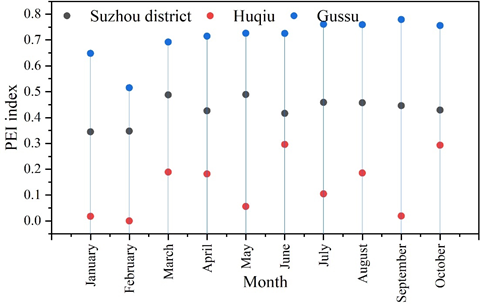
Through the above analysis, it is concluded that the case density has a certain impact on the accuracy of case prediction, so on the basis of the citywide prediction, two areas with different case densities are selected for comparative analysis. In this paper, Gusu District with higher case density and Huqiu District with lower case density are selected to calculate the PEI index of their local prediction and analyze it in comparison with the number of cases.
Figure 7 shows the PEI index of crime prediction in different regions, and it can be visualized from the figure that the PEI index of crime prediction in each month is higher in Gusu district than in Suzhou citywide, and the 10-month PEI mean values of crime prediction for both of them are 0.7076 and 0.4303 respectively, and they are similar in terms of accuracy. The accuracy of both Gusu District and Suzhou citywide is much higher than the prediction accuracy of Huqiu District (0.1343), and this trend is in the same order of magnitude as the density of these three cases.
In this paper, based on the graph self-encoder model, the adaptive graph learning module, self-attention module and objective function are constructed, combined with the GRU model to form a graph self-encoding recurrent neural network, and spatio-temporal environment elements are introduced to complete the establishment of the spatio-temporal prediction model of crime. Subsequently, the prediction results of the model are verified, and the model is applied to realize crime prediction for cases in different months, time periods and regions.
Using the GAERNN algorithm, the prediction performance of each modality is evaluated hierarchically for 78 communities, and the prediction \(R^{2}\) of all mode sets except M8 is above 0.9. After summing all modalities by corresponding nodes, the \(R^{2}\) value is 0.795484, and the MAE, MSE, and RMSE are 0.035984, 0.001987, and 0.043985, respectively. The model is capable of capturing the spatio-temporal dependence of low and medium frequency neighborhood crimes. For the comparison of the absolute errors of prediction of the number of theft, assault, battery, and criminal damage cases, the model optimized with the introduction of spatio-temporal environmental elements has an absolute error of prediction of no more than 0.05.
By comparing the two types of crime prediction algorithms and evaluating the prediction effect on the cases of property invasion in different months, the GAERNN algorithm’s hit rate is higher than or equal to the IsotDM algorithm.In the two crime risk levels of very high risk and high risk, the hit rate of the IsotDM algorithm is only 7.3% and 14.58%, with an average PEI index of 13.35 and 12.15, respectively.The GAERNN algorithm introduces the geographic unit in which the case is located, which is 20.98% and 25.77%. The GAERNN algorithm, on the other hand, had an average hit rate of 20.98% and 25.77%, with PEI metrics of 36.96 and 24.22, respectively.The GAERNN algorithm introduces environmental similarities in the geographic units in which the cases are located, adding dimensions to the assessment of crime risk.
Conflict of interest: The authors declare that they have no conflicts of interest.