
In today’s increasingly prosperous and complex financial markets, financial markets have experienced unprecedented rapid development and numerous product innovations, providing investors with richer and more diversified choices [12,20]. Such rapid development and innovation also bring challenges in pricing and risk assessment, and traditional methods are difficult to adapt to the complex and changing market environment in the face of the fast market environment and massive data, to the extent of failing to meet the demand for high precision and efficiency [16]. Therefore, it is especially important to explore and apply new technical means, especially the introduction and application of artificial intelligence technology. With its powerful data processing capability and pattern recognition ability, AI technology can improve the precision and efficiency of pricing, while enhancing the timeliness and accuracy of risk assessment, thus ensuring the stability of the financial market [1,17].
Zhang,Y. mainly discussed the value of application in financial derivatives pricing to improve the efficiency and accuracy of Monte Carlo simulation through variance reduction technique to achieve the optimization of financial derivatives pricing model [22]. Wu, J et al. proposed a prediction method combining convolutional neural network and long and short-term memory network for investment financial products. The historical data of investment products are used as a sequence group to extract the product feature vectors and improve the prediction performance [19]. Levin, P proposed a pricing model that combines forward and backward stochastic differential equations while considering the dynamic evolution of the asset price and the expected return or boundary conditions at the terminal moment. In finance, idiosyncratic noise usually refers to unsystematic risk factors associated with a particular asset or firm. By incorporating these idiosyncratic factors into the pricing model, using a forward-backward stochastic model and incorporating idiosyncratic noise, the actual value of financial assets can be more accurately reflected between [10]. He,W. and Guan,M. utilized the powerful feature extraction capability of CNNs to automatically learn and identify the key factors affecting the price of options from high-frequency trading data. It not only avoids the limitation of manually setting parameters and assumptions in traditional models, but also captures the hidden information in the market microstructure, thus reflecting the market value of options more accurately [8].
In the process of risk assessment, scholars actively utilize advanced technological tools such as big data analysis, artificial intelligence, and machine learning. These tools can improve the accuracy and efficiency of risk assessment.Pons, A et al. studied the prediction of value-at-risk as a measure of the risk of investment loss in financial products. Using the profitability extrapolation function, a skewed Student-tGARCH(1,1) model was used for assessment at the single product level, and a t-copula model was used to complete the interdependence assessment at the portfolio level [13]. Han, D. proposed a risk assessment framework based on factor analysis, which is capable of systematically assessing the risk in the pricing models of financial products . A firm-level financial risk evaluation model was developed to determine the extent of the model’s impact on solvency, operating ability, profitability, development ability, and the ability to obtain cash flow By analyzing and identifying key risk factors, the framework may help investors and managers better understand financial risks and formulate risk management strategies accordingly [6]. Qu,X on the basis of analyzing intelligent optimization algorithms constructed a set of effective credit risk assessment model for financial data, by introducing intelligent optimization algorithm to intelligently select and assign weights to the features in financial data, so as to construct a more accurate and stable credit risk assessment model. The application of intelligent optimization algorithm not only improves the assessment accuracy of the model, but also adaptively adjusts the model parameters to adapt to the ever-changing market environment [21]. Zhang,H. proposed the theory of the impact of big data on the evaluation of corporate financial risk, which incorporates the big data public opinion indicators into the traditional corporate financial risk evaluation indicators. The empirical results were obtained using fuzzy hierarchical analysis. A framework combining big data technology and FAHP is used to more accurately assess and quantify corporate financial risk, and thus optimize financial product pricing models. It helps financial institutions and investors to better consider risk factors when developing pricing strategies [15].
This study aims to explore how to optimize financial product pricing models and improve risk assessment methods using artificial intelligence technology. Firstly, a financial product customer segmentation model and a product relevance analysis model are established through customer data mining to provide data support for pricing. Next, the depreciation rate and customization degree of data products are introduced into the dynamic utility functions of supply and demand, and the data product pricing models of member firms are constructed for the two market situations of single-attribution and partial-multiple-attribution, respectively, and the pricing strategies of data products are formulated. Finally, a systematic financial risk assessment system is constructed, including the construction of the financial risk indicator system and the division of the principal component analysis and financial risk early warning state.
This paper establishes a customer segmentation model based on the X-means clustering algorithm starting from multiple elements such as gender, age, occupation and annual income. First, customer historical transaction data are collected and screened and analyzed, and the search range of clustering parameter \(R\) is determined based on the experience of domain experts \(\left[R{\rm 1},R{\rm 2}\right]\). After finding the optimal clustering number \(R\), each characteristic data corresponding to each clustering number is analyzed to construct the customer segmentation model [2]. Financial product customer segmentation is shown in Table 1, according to the customer segmentation results corresponding to the cluster number, it can be judged that a certain type of customers tend to buy a certain type of financial products. Therefore, for customers who meet the characteristics of a certain category, corresponding marketing strategies can be adopted. In terms of association strength, the number of all customers who have purchased product \(i\) is counted and set to \(K_{i}\). Then the number of these \(K_{i}\) customers who have purchased product \(j\) is counted and set to \(K_{j}\). \(R_{ij} =K_{j} /K_{i}\) is the association strength between product \(i\) and product \(j\), and \(R_{ij}\) shows how probable it is that a customer who has purchased product \(i\) will purchase product \(j\).
| Cluster Sequence | Weighting | Male to female ratio | Age Span | Occupation | Annual Income | Transaction Span |
| 1 | N1 | B1:G1 | A0,A1 | P1 | I1 | T0,T1 |
| 2 | N2 | B2:G2 | A1,A2 | P2 | I2 | T1,T2 |
| R | NR | BR:GR | AR-1,AR | PR | IR | TR-1,TR |
Product relevance is shown in Table 2, according to the customer clustering analysis and product relevance analysis, customer characteristics are summarized and described to form a customer pair. According to the strength of product association can be judged that the customer after purchasing product \(j\), often tends to buy product \(k\), then after the customer purchases product \(j\) can be cross-marketed to its product \(k\), greatly improving the success rate of combination sales or cross-selling [9]. According to the customer’s basic information, name, age annual income, occupation, etc. and the results of customer segmentation, to determine the classification to which the customer belongs, and according to the characteristics of the class of customers to determine the bias of their consumption. Through the product relevance analysis to reveal the potential connection between different customer groups, more accurately determine the market demand, for the subsequent market actual pricing strategy to provide strong support.
| Relevance | Product 1 | Product 2 | Product N | |
| Product 1 | 1 | R12 | R1N | |
| Product 2 | R21 | 1 | R2N | |
| … | 1 | |||
| Product N | RN1 | RN2 | 1 |
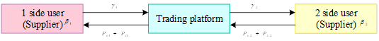
In this paper, the Hotelling model is used to study the data product pricing model in two cases, i.e., single-attribution and partial-multi-attribution for both supply and demand-side firms, respectively. Consider members only join a big data industry, that is, within the demand side and the supply side all join in a monopoly trading platform for trading, at this time no need to consider the platform difference problem. Assuming that the platform is profit-maximizing, the platform adopts a two-step charging system for both sides, and Figure 1 shows the market structure with single attribution of the supply-side firms. \(\gamma _{1}\) and \(\gamma _{2}\) denote the intergroup network externality parameters of demand-side firms to supply-side firms and supply-side firms to demand-side firms \(\left(\gamma _{1} ,\gamma _{2} >0\right)\), \(\beta _{1}\) and \(\beta _{2}\) denote the intragroup network externality parameters of users on both sides of the platform \(\left(\beta _{1} ,\beta _{2} >0\right)\), and \(P_{s1}\) and \(P_{s2}\) denote the fees charged by the platform to households on both sides of the platform [7]. \(P_{t1{\rm \; }}\) and \(P_{t2}\) denote the transaction fees charged by the platform to the supply-side and demand-side users in each transaction, assuming that the transaction fees charged by the platform are calculated on the basis of the total amount of each transaction. \(n_{1}\) and \(n_{2}\) denote the number of supply-side and demand-side users on both sides of the platform, and \(n_{1}\) and \(n_{2}\) are also functions of \(u_{1}\) and \(u_{2}\), such that \(n_{1} =\varphi _{1} \left(u_{1} \right)\), \(n_{2} =\varphi _{2} \left(u_{2} \right)\).
The utility of member firms’ access to the platform is respectively: \[\label{GrindEQ__1_} \left\{\begin{array}{l} {u_{1} =\gamma _{1} n_{2} -\beta _{1} n_{1} -P_{s1} }, \\ {u_{2} =\gamma _{2} n_{1} -\beta _{2} n_{2} -P_{s2} }.\end{array}\right. \tag{1}\]
The utility gained by a member firm from single attribution on one side of the platform is equal to the network externality effect gained by that member firm from joining the platform, multiplied by the number of member firms on the other side of the platform, minus the member firm’s intra-group network externality within the platform, and then multiplied by the number of member firms on the platform’s own side, minus the registration fee charged by the platform. Indications \(\gamma _{1} n_{2}\) and \(\gamma _{2} n_{1}\) represent the increased benefits of an enterprise joining the platform under the influence of the inter-group network externality, and indications \(\beta _{1} n_{1}\) and \(\beta _{2} n_{2}\) represent the reduced benefits of an enterprise under the influence of the intra-group network externality on its own side of the platform. Denote \(n_{1}\) and \(n_{2}\):
\[\label{GrindEQ__2_} \left\{\begin{array}{l} {n_{1} =\frac{\gamma _{1} n_{2} -P_{s1} -u_{1} }{\beta _{1} } =\varphi _{1} \left(u_{1} \right)}, \\ {n_{2} =\frac{\gamma _{2} n_{1} -P_{s2} -u_{2} }{\beta _{2} } =\varphi _{2} \left(u_{2} \right)}. \end{array}\right. \tag{2}\]
The optimal pricing strategy of the platform is obtained by solving the first-order condition for profit maximization of the platform: \[\label{GrindEQ__3_} \left\{\begin{array}{l} {P_{s1} =-\gamma _{2} n_{2} +\beta _{1} n_{1} +\frac{\varphi _{1} \left(u_{1} \right)}{\varphi _{u_{1} } \left(u_{1} \right)} }, \\ {P_{s2} =-\gamma _{1} n_{1} +\beta _{2} n_{2} +\frac{\varphi _{2} \left(u_{2} \right)}{\varphi _{u_{2} } \left(u_{2} \right)} }. \end{array}\right. \tag{3}\]
The expected utility function of the demand side to purchase the data product considering the loss of value and the degree of customization of the product [11]. The expression is: \[\label{GrindEQ__4_} u_{x} =\left(\gamma _{2} n_{1} -\beta _{2} n_{2} \right)v-P-P_{s2} -P_{t2} . \tag{4}\]
In the case of equilibrium between the two sides of the product production and demand, so that the supply and demand side of the enterprise utility consistent solution to the product demand for: \[\label{GrindEQ__5_} Q=\frac{P_{ss1} -P_{ss2} +u_{x} }{\left(\gamma _{1} n_{2} -\gamma _{2} n_{1} +\beta _{2} n_{2} -\beta _{1} n_{1} \right)\xi +2P} . \tag{15}\]
Under the condition of single attribution of firms corporate profits are generated only in one trading platform, when the corporate profit function is: \[\label{GrindEQ__6_} \pi =PQ . \tag{6}\]
Under the objective of profit maximization of the firm, the product pricing \(P\) can be obtained as: \[\label{GrindEQ__7_} P=\frac{\sqrt{X^{2} -2X\left(P_{ss1} -P_{ss2} +\left(\gamma _{2} n_{1} -\beta _{2} n_{2} \right)\xi e^{-\lambda t} \right)} -X}{2} . \tag{7}\] where \(X=\left(\gamma _{1} n_{2} -\gamma _{2} n_{1} +\beta _{2} n_{2} -\beta _{1} n_{1} \right)\xi e^{-\lambda t}\). It can be seen that the price of a data product decreases gradually with its depreciation rate and over time, and that data products and prices are inversely proportional to their timeliness and degree of customization.
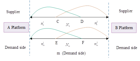
The standard Hotelling model framework is also used to analyze the pricing behavior of the supply-side firms when some of the member firms in the trading platforms belong to more than two platforms. The relationship between the platforms and the member firms on both sides is shown in Figure 2, assuming that both platforms \(A\) and \(B\) adopt a two-step charging system at line segment [0.1], and that the users on both sides of the platforms, supply-side and demand-side, \(k\) and \(m\), are uniformly distributed and partially multi-attributed on the line segment. With oligopolistic price competition on both sides of the platform, the intergroup network externality coefficients for platforms \(A\) and \(B\) are \(\gamma _{1}\) and \(\gamma _{2}\), respectively, and the intragroup network externality coefficients are \(\beta _{1}\) and \(\beta _{2}\), and the number of single-attributed subscribers on one side of the user group \(k\) on platforms \(A\) and \(B\) are \(n_{k}^{1}\) and \(n_{k}^{2}\), respectively, and the number of partially multi-attributed subscribers is \(N_{k}\). The user size is standardized to 1 for both, i.e., \(n_{k}^{1} +n_{k}^{2} +N_{k} =1\), \(P_{i}^{sj}\) as the registration fee for firms to enter the two platforms, and \(P^{tj} {}_{i}\) as the transaction fee paid by firms in each transaction \((i=k,m,j=A,B)\) [4].
\(k\) Net utility at multiple vesting is: \[\label{GrindEQ__8_} u_{k}^{12} =\gamma _{1} n_{m}^{1} +\gamma _{2} n_{m}^{2} +\frac{\left(\gamma _{1} +\gamma _{2} \right)}{2} N_{m} -\beta _{1} \left(n_{k}^{1} +N_{k} \right)-\beta _{2} \left(n_{k}^{2} +N_{k} \right)-P_{k}^{sA} -P_{k}^{s\; B} -1 . \tag{8}\]
There exist critical points \(C,D,E\) and \(F\) for user groups \(k\) and \(m\) on both sides of the platform, respectively, such that users have the same utility in choosing either single-attribution or multi-attribution at the critical points, which can be obtained by ordering \(u_{k}^{1} =u_{k}^{12} ,\quad u_{k}^{2} =u_{k}^{12}\), respectively: \[\label{GrindEQ__9_} \left\{\begin{array}{l} {C=1-\gamma _{2} n_{m}^{2} +\frac{\left(\gamma _{1} -\gamma _{2} \right)}{2} N_{m} +\beta _{2} \left(n_{k}^{2} +N_{k} \right)+P_{k}^{s\; B} }, \\ {D=1-\gamma _{1} n_{m}^{1} +\frac{\left(\gamma _{2} -\gamma _{1} \right)}{2} N_{m} +\beta _{1} \left(n_{k}^{1} +N_{k} \right)+P_{k}^{sA} }. \end{array}\right. \tag{9}\]
Since \(n_{m}^{1} +n_{m}^{2} +N_{m} =1\), according to the Hotelling model, the left side of point \(C\) is for firms in \(k\) that are single-attributed to platform \(A\), and the right side of point \(D\) is for firms in \(k\) that are single-attributed to platform \(B\), let \(C=n_{k}^{1} ,D=n_{k}^{2}\) and the platform revenue function under the consideration of firms’ initial entry into the platform and payment of registration fees only is: \[\label{GrindEQ__10_} \left\{\begin{array}{l} {\pi _{A} =P_{k}^{sA} \left(1-n_{k}^{2} \right)+P_{m}^{s\; {\rm A}} \left(1-n_{m}^{2} \right)}, \\ {\pi _{B} =P_{k}^{s\; {\rm B}} \left(1-n_{k}^{1} \right)+P_{m}^{s\; {\rm B}} \left(1-n_{m}^{1} \right)}. \end{array}\right. \tag{10}\]
Under the conditions of symmetric platform prices and profit maximization, solve for the platform’s registration fee for user group \(k,m\): \[\label{GrindEQ__11_} \left\{\begin{array}{l} {P_{k}^{s\; {\rm A}} =P_{k}^{s\; {\rm B}} =\gamma _{1} \gamma _{2} -2\gamma _{1} -2\gamma _{2} -\gamma _{1}^{2} -\beta _{2} +\beta _{1} } \\ {P_{m}^{s\; {\rm A}} =P_{m}^{s\; {\rm B}} =\gamma _{1} \gamma _{2} -2\gamma _{1} -2\gamma _{2} -\gamma _{2}^{2} -\beta _{1} +\beta _{2} } \end{array}\right. \tag{11}\]
The demand-side enterprise’s demand for a particular data product can only be obtained from one transaction platform, and considering the transaction fee paid by the enterprise in each transaction, let the demand-side’s expected utility function of the data product on platforms \(A\) and \(B\), respectively [3]. The expression is: \[\label{GrindEQ__12_} \left\{\begin{array}{l} {u^{A} =\gamma _{1} \left(1-n_{k}^{2} \right)\xi -\beta _{1} \left(1-n_{m}^{2} \right)v-P_{A} -P_{m}^{sA} -P_{m}^{{\rm tA}} } \\ {u^{B} =\gamma _{2} \left(1-n_{k}^{1} \right)\xi -\beta _{2} \left(1-n_{m}^{1} \right)v-P_{B} -P_{m}^{s\; {\rm B}} -P_{m}^{{\rm tB}} } \end{array}\right. \tag{12}\]
Assuming \(P_{A}\) and \(P_{B}\), the product price for the product supply side of the two platforms, \(k\) and \(m\) join the same base utility of the two platforms, \(Q_{A}\) and \(Q_{B}\). for the base utility of the supply side and the demand side and the demand for the product, so that the supply and demand side of the platforms on both sides of the enterprise utility is the same, solving for the utility function of the two enterprises through the platforms to carry out the transaction of the data products solving for the demand for the product is: \[\label{GrindEQ__13_} \left\{\begin{array}{l} {Q_{A} =\frac{P_{mmk}^{{\rm A}} -P_{mmm}^{{\rm A}} +u_{x}^{A} }{\left(\gamma _{1} +\beta _{1} \right)\left(n_{k}^{2} -n_{m}^{2} \right)v+2P_{A} } } \\ {Q_{B} =\frac{P_{mmk}^{{\rm B}} -P_{mmm}^{{\rm B}} +u_{x}^{B} }{\left(\gamma _{2} +\beta _{2} \right)\left(n_{k}^{1} -n_{m}^{1} \right)v+2P_{B} } } \end{array}\right. \tag{13}\]
In the enterprise part of the conditions of multiple attribution of corporate profits have two kinds of generation, single attribution of corporate profits in one generation, multiple attribution of corporate profits in two generation, at this time the corporate profit function is: \[\label{GrindEQ__14_} \pi ^{k} =\pi _{k}^{A} +\pi _{k}^{B} =P_{A} Q_{A} +P_{B} Q_{B} \tag{14}\]
available with the goal of maximizing corporate profits: \[\label{GrindEQ__15_} \left\{\begin{array}{l} {P_{A} =\frac{\sqrt{Y^{2} -2Y\left[P_{mmk}^{{\rm A}} -P_{mmm}^{{\rm A}} +\gamma _{1} \left(1-n_{k}^{2} \right)\xi e^{-\lambda t} -\beta _{1} \left(1-n_{m}^{2} \right)\xi e^{-\lambda t} \right]} -Y}{2} } \\ {P_{B} =\frac{\sqrt{Z^{2} -4Z\left[P_{mmk}^{{\rm B}} -P_{mmm}^{{\rm B}} +\gamma _{2} \left(1-n_{k}^{1} \right)\xi e^{-\lambda t} -\beta _{2} \left(1-n_{m}^{1} \right)\xi e^{-\lambda t} \right]} -Z}{2} } \end{array}\right. \tag{15}\] where, \(Y=\left(\gamma _{1} +\beta _{1} \right)\left(n_{k}^{2} -n_{m}^{2} \right)\xi e^{-\lambda t}\), \(Z=\left(\gamma _{2} +\beta _{2} \right)\left(n_{k}^{1} -n_{m}^{1} \right)\xi e^{-\lambda t}\). It can be seen that the price of the data product decreases gradually with its depreciation rate and time, i.e., the data product and price are inversely proportional to its timeliness and customization [14]. When the supply-side firm joins \(f\) trading platforms, the final data product pricing at the \(g\)th platform is: \[\label{GrindEQ__16_} P=\sqrt{W^{2} -2W\left[P_{mmk}^{{\rm g}} -P_{mmm}^{{\rm g}} +\gamma _{g} \left(1-\sum _{h=1}^{g-1}n_{k}^{h} \right)\xi e^{-\lambda t} -\beta _{g} \left(1-\sum _{h=1}^{g-1}n_{m}^{h} \right)\xi e^{-\lambda t} \right]-W},\;\; (2\le g\le f) \tag{16}\] where \(\gamma _{g}\) and \(\beta _{g}\) are the inter-group network externality and intra-group network externality of the supply-side firm on the \(g\)rd trading platform, \(n_{k}^{h}\) and \(n_{m}^{h}\) are the number of single-attributed users of the supply-side firm and the demand-side firm on the non-\(g\) platform, and \(P_{k}^{tg}\) and \(P_{m}^{tg}\) are the transaction costs of the supply-side firm and the demand-side firm on the non-\(g\) platform, respectively. Special, when \(f=1\), i.e., when firms join only one platform for trading. Eq. holds under conditions \(\gamma _{1} =\gamma _{2}\), \(\beta _{1} =\beta _{2}\) due to the consideration of the effect of network externalities between the two groups of supply and demand side firms within the platform.
Table 3 shows the evaluation indicators for financial risk assessment and early warning, which comprehensively consider several economic dimensions to ensure the comprehensiveness and sensitivity of the indicator system. Starting from the core aspects of economic growth, fiscal security, monetary expansion, bubble accumulation, and banking system soundness, key indicators that can reflect the risk status in these areas are selected [18]. In constructing this indicator system, inspired by the Hotelling model, the same attention needs to be paid to the timeliness and customization of the indicators to ensure the accuracy and effectiveness of the early warning system.
| Types of Risks | Early warning indicators | Qualitative description of the relationship between indicators and financial risk |
| Economic stability risk | GDP growth rate (X1) | There is a risk of overheating the economy or the emergence of a recession. |
| Level of social fixed investment (X2) | Low investment is a precursor to recession and crisis. | |
| Inflation level (X3) | Reflects the effectiveness of monetary policy and the value of real money. | |
| Fiscal Risk | Fiscal deficit(X4) | Reflects the extent to which government finances are insufficient. |
| Fiscal Dependency(X5) | Reflects the extent to which the government’s financial resources are adequate. | |
| National debt burden level(X6) | Reflects the ability of the national economy to withstand the national debt. | |
| Currency Risk | Size of Credit(X7) | Excessive credit expansion is prone to accumulate liquidity risk. |
| M2 expansion rate(X8) | Excessive expansion leads to excess liquidity and speculative risks. | |
| Real interest rate(X10) | Reflecting the level of financial liberalization, too high a level can trigger speculative risks. | |
| Bubble Risk | House price growth rate(X11) | Accumulation of real estate bubble risks can be transmitted to the financial system. |
| Securitization level(X12) | Reflects market investment opportunities and the degree of bubble accumulation. | |
| Equity P/E ratio(X13) | Reflects the bubble situation in the stock market. | |
| Banking System Risk | Bank capital-to-asset ratio(X14) | Reflects the stability of banks and their ability to pay off their liabilities. |
| Bank Liquidity Ratio(X15) | Measures the degree of liquidity risk in the banking system. | |
| Bank Non-Performing Loan Ratio(X16) | Non-performing loan monitoring is key to the sound operation of the banking system. |
The systematic financial risk evaluation index system constructed in this paper contains 16 economic and financial indicators that are closely related to risk accumulation. In order to comprehensively assess the state of financial risk, further standardization of the indicators is carried out, according to the relationship between the indicators and systemic financial risk can be divided into positive indicators, negative indicators and moderate indicators, and the indicators of different natures are standardized with Z-score standardization, inverse positive and threshold standardization, etc., and the process is completed using MATLAB 7.0.
In order to improve the training efficiency of the model in this paper, principal component analysis is used to downscale the selected samples, extract the main factors affecting financial risk and use them to classify the financial risk warning status. Further, based on the basic principle that the eigenvalue is greater than, four principal factors closely related to financial risk are extracted to evaluate the systemic financial risk status from the following four aspects:
The principal factors load the indicators of monetary and banking security.
The main factor loaded indicators on economic growth and balance of payments.
The main factor loads on external shock indicators.
The main factor loaded indicators on fiscal and bubble risk [5].
Further weighted average of the variance contribution rate of the four main factors can get the comprehensive indicators reflecting the early warning status of financial risk, and complete the assessment and classification of financial risk.
To compare the prediction effect of Hotelling model in this paper, the experiment will be conducted separately for call and put options. Among them, the call option data totaled 41,481 lines and the put option data 43,583 lines, and the first 4506 lines of data of each option are used as the training set, and the remaining data are used as the test set. A total of 240 call option price predictions and 360 put option price predictions are obtained. According to the characteristics of 50ETF options, the inputs of the model are 50ETF opening price S, for the option expiration execution price K, 6-month treasury bond yield r, option expiration time/365T, and 90-day historical volatility sigma. The output of the model is the option prediction value, which is denoted by P. The model is based on the model’s output. The loss function judgment criterion uses mean square error, and the parameter learning algorithm uses stochastic gradient descent, with each mini-batch set to 30.
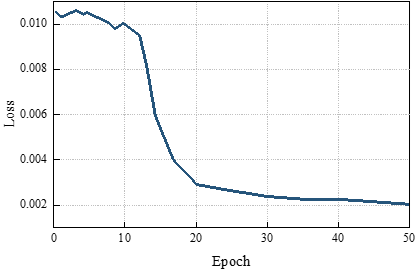
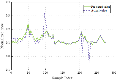
Figure 3 shows the model call option pricing prediction in this paper, Figure 3(a) shows the change of loss in the training set, when Epoch=10, the loss function began to have a tendency to converge, but after that, the loss declined rapidly. the loss function gradually showed a tendency to converge when Epoch=40. And with the increase of the number of iterations, the loss value tends to be stable, which indicates that the model gradually converges in the training process, and the optimization effect gradually appears. Figure 3(b) shows the comparison between the predicted value and the real value, the predicted value has been able to fit the real value better, which further verifies the effectiveness of the model. When the sample index is 260, the normalized price predicted by the model call option pricing in this paper is 0.154 with the true value of 0.153, which is a high degree of fit, and the model gradually learns the information contained in the data and is able to accurately predict the price of the call option. This shows that the model’s generalization ability gradually improves and is able to make accurate predictions on new and unseen data, which fully demonstrates the excellent performance of this paper’s model in call option pricing prediction.
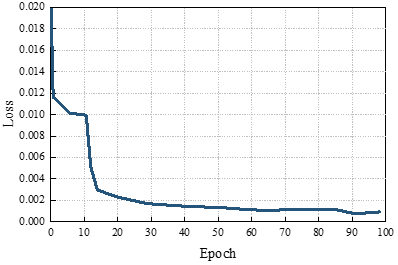
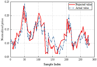
In order to continue to verify the prediction ability of the pricing strategy based on the Hotelling model, put option pricing prediction experiments are conducted. In the case of Epoch=50, the put option pricing prediction of this paper’s model is shown in Figure 4. Figure 4(a) shows the change in the loss of the training set, and it can be seen that the loss function no longer decreases when Epoch=100, indicating that the model has converged. Figure 4(b) shows the comparison of the predicted value and the true value, using the predicted value generated by the converged model can fit the true value very well, the sample index is 50, this paper’s model call option pricing prediction of the normalized price of 0.237, the true value of 0236. the sample index is 200, this paper’s model call option pricing prediction of the normalized price of 0.146, the true value of 0.145, the two The data are highly fitted, indicating that the model in this paper has a good ability to predict option prices.
In order to make a multi-dimensional comparison, the underlying historical volatility is added to the input variables. The measures are MAPE and RMSE for out-of-sample forecasts, and Figure 5 shows the comparison of pricing error models for financial products. The results of the comparison are as follows:
The option pricing model has a pricing error of 0.041, which may be more difficult for the average consumer to understand and more costly to implement. The auction pricing model has a pricing error of 0.0295, which leads to higher price volatility and requires higher transaction costs. The out-of-sample pricing error of the cost-plus pricing model is 0.0294, which fails to fully consider the market demand and competitive environment deviating from the optimal price.
The skimming pricing model targets high-end consumers with high prices, and the out-of-sample pricing error is 0.0281. High profits can be realized in the short term, but sustainability may be affected in the long term due to limited market share and loss of consumers. The dynamic pricing model adjusts prices according to real-time changes in the market, with a pricing error of 0.0276. It is able to react quickly to market fluctuations, but may require a high level of data analysis and processing power.
The pricing model based on game theory takes into account the strategic interactions between market participants, with a pricing error of 0.0265. It is able to predict the behavior of competitors and formulate the optimal pricing strategy accordingly. The market-oriented pricing model bases its pricing on market demand and competitive conditions. In the sample data, the pricing error of this model is 0.0261. it relies too much on market signals, resulting in large price fluctuations in some cases Psychological pricing model utilizes customers’ psychological factors for pricing, such as tail pricing and integer pricing, etc., and the out-of-sample pricing error is 0.0243. it is effective in attracting customer’s attention and facilitating purchases, but the effect may vary depending on the market and the group of consumers.
The value pricing model is based on the customer’s perception of the value of the product to price, the pricing error of the model is 0.0232, which is the lowest among all models except the model in this paper. It shows that it can accurately reflect the customer’s perception of the value of the product, so as to set a more attractive price. The pricing model in this paper comprehensively considers various factors such as market, cost, competition and consumer behavior, and the out-of-sample pricing error is only 0.0214. It performs well in a variety of market environments and can flexibly cope with different situations, showing significant superiority and practicality.

The risk assessment results of the financial risk early warning model are shown in Table 4. The model in this paper effectively predicts several systemic financial risk indicators in 2020 and 2022, and the predicted values are relatively close to the actual values.The actual value of the GDP growth rate X1 was 7.01% in 2017, and 6.68% in 2018, which shows the trend of slowing down of the economic growth rate. The model predicted values are similar to the actual values, indicating that the model has high accuracy in predicting the GDP growth rate. The risk status is assessed as medium risk, indicating that the economic growth rate, although slowing down, is still within the controllable range. The level of social fixed investment, X2, was 45.2% in real terms in 2017 and 43.8% in real terms in 2018, indicating a slight decline in the level of investment. The model’s forecasts of 45.1% and 43.9% for the two years are highly consistent with the actual values. Inflation level X3, with actual values of 3.5% in 2017 and 3.7% in 2018, showed a slight increase in inflation. The model’s predicted values of 3.6% and 3.8%, respectively, indicate a relatively stable level of inflation. Fiscal deficit X4 risk status is assessed as medium risk, indicating that an increase in the fiscal deficit may have some impact on fiscal stability. Fiscal Dependence X5, with a risk status assessed as medium risk, indicates that changes in fiscal dependence need attention. National debt burden level X6, with an actual value of 65.0% in 2017 and 67.5% in 2018, shows a significant increase in the level of national debt burden.
| Norm | 2021 Actual | 2022 Actual | 2021 Forecast | 2022 Forecast | Risk Status Assessment |
| (X1) | 7.01% | 6.68% | 6.99% | 6.67% | Medium Risk |
| (X2) | 45.2% | 43.8% | 45.1% | 43.9% | Medium Risk |
| (X3) | 3.5% | 3.7% | 3.6% | 3.8% | Low Risk |
| (X4) | 2.8% | 3.1% | 2.9% | 3.0% | Medium Risk |
| (X5) | 30.5% | 32.0% | 30.8% | 31.9% | Medium Risk |
| (X6) | 65.0% | 67.5% | 64.8% | 67.3% | High Risk |
| (X7) | 150.0% | 155.0% | 149.5% | 154.8% | High Risk |
| (X8) | 12.0% | 11.5% | 11.8% | 11.3% | Medium Risk |
| (X10) | 4.0% | 3.8% | 3.9% | 3.7% | Low Risk |
| (X11) | 8.5% | 9.0% | 8.4% | 8.9% | Medium Risk |
| (X12) | 55.0% | 57.5% | 54.8% | 57.3% | Medium Risk |
| (X13) | 18.0 | 19.5 | 17.8 | 19.3 | Medium Risk |
| (X14) | 9.0% | 8.8% | 8.9% | 8.7% | Low Risk |
| (X15) | 40.0% | 38.5% | 39.8% | 38.3% | Medium Risk |
| (X16) | 2.0% | 2.2% | 1.9% | 2.1% | Low Risk |
The predicted values of the model are 64.8% and 67.3% respectively, which are very close to the actual values. The risk status is assessed as high risk, and the rising level of national debt burden is a serious risk point. Credit Scale X7 the risk status is assessed as high risk, and the rapid expansion of credit scale may bring systemic risk. The M2 expansion rate X8 risk status is assessed as medium risk, with changes in the M2 expansion rate requiring attention. Real interest rate X10 risk status is assessed as low risk, indicating that the real interest rate is at a reasonable level. House price growth rate X11 risk status is assessed as medium risk, the rapid growth of house price may bring potential risk. Securitization level X12 Risk status is assessed as medium risk, and changes in securitization level need to be watched. An increase in the equity P/E ratio X13 may reflect an overheated market. Bank Capital to Asset Ratio X14 the risk status is assessed as low risk, indicating that the bank’s capital adequacy ratio is at a reasonable level. Bank Liquidity Ratio X15 the risk status is assessed as medium risk and changes in bank liquidity need to be watched. The risk status is assessed as low risk, indicating that the bank’s capital adequacy ratio is at a reasonable level. Bank NPL ratio X16 The actual value of the bank NPL ratio was 2.0% in 2017 and 2.2% in 2018, the bank NPL ratio has increased The risk status is assessed as low risk, indicating that the bank’s NPL ratio is at a low level. However, it is still necessary to pay attention to the trend of its change, the model has a certain degree of accuracy and usefulness in forecasting and risk assessment.
This study establishes a financial product customer segmentation model and a product relevance analysis model through customer data mining to provide data support for pricing. Considering the different attribution of supply-side and demand-side enterprises, a systematic financial risk indicator system will be constructed, and the principal component analysis method will be used to classify the early warning status of financial risk, providing new ideas and methods for risk assessment. The conclusions are as follows:
In call option pricing prediction, the proposed model performs well, and the loss function starts to converge at Epoch=40 and reaches a stable state at Epoch=50. The predicted value is highly fitted to the true value, e.g., when the sample index is 260, the predicted price is 0.154 and the true value is 0.153.
In put option pricing prediction, the proposed model also shows good predictive ability. The loss function converges at Epoch=100, and the predicted value is highly consistent with the true value, e.g., when the sample index is 50, the predicted price is 0.237, and the true value is 0.236, which shows the model’s ability to accurately predict the price of options.
The model proposed in this paper outperforms the other nine comparative models in both RMSE and MAPE performance, with an out-of-sample pricing error of only 0.0214. At the same time, the model has a high prediction accuracy, identifying the level of the national debt burden X6 and the size of the credit X7 as high-risk points that require special attention.