
The distribution network is directly connected to the users located at the end of the power system, and a sudden fault will cause a power outage and have a significant negative impact [13]. With the large penetration of distributed generation (DG) in the power system, how to utilize distributed power to restore power in outage areas has become a research hotspot in smart grid studies. Wind and photovoltaic power generation are now widely used as clean distributed power sources, but their output is uncertain due to their dependence on environmental conditions [4]. To maximize the application of DG, energy storage devices are often built in the distribution network to better absorb wind and photovoltaic power through charging and discharging. However, DG’s characteristics of randomness, volatility, and intermittency may lead to power outages in restored areas, causing significant user losses. Therefore, improving the utilization of DG has become an urgent research focus [5].
At present, many scholars have studied the fault recovery problem in distribution networks containing DG, with mainstream research approaches including heuristic search, mathematical programming, and intelligent optimization algorithms [7]. Heuristic rules were among the early algorithms applied to fault recovery in distribution networks [1]. By formulating specific switching and transformation rules, the optimal network structure can be restored in non-fault areas [11]. For instance, some studies adjust the switches based on real-time fault status and restore the network through reconstruction [8]. In distribution networks containing distributed photovoltaics, flexible soft switches (SOPs) have been used instead of mechanical switches, supplemented by photovoltaic forecasting to achieve fault recovery [6]. This approach uses electronic means to enhance action speed. Other studies propose the concept of static stability margin for islands and construct hierarchical distributed decision-making systems using multi-agent technology to coordinate DG outputs in islands [9]. Furthermore, various distributed energy-coupled networks have been constructed to enable the transfer of load energy types between systems, allowing for active disconnection during faults and studying its impact [12]. Fault recovery can be treated as a nonlinear multi-objective and multi-constraint problem. Intelligent algorithms, with their parallel processing and global search capabilities, have been widely applied to solve such problems. For instance, combining two algorithms has been proposed as an effective way to avoid one algorithm falling into local optimization [3]. However, the existing research has the following issues:
1. The temporal variability of DG output is not well integrated with the temporal changes in load during power supply restoration.
2. The active adjustment capabilities of the user-side load are not considered in determining the recovery sequence of faulty nodes.
To address these issues, this paper first establishes a distribution network model with DG and considers the demand response of user-side loads. When a fault occurs, the network traversal method is used for island division, prioritizing the recovery of nodes with high load levels. Subsequently, the whale optimization algorithm is employed to reconstruct the remaining non-faulty power loss areas to obtain the optimal recovery strategy. Finally, the improved IEEE33 node system is simulated and verified.
The output power of wind power generation is closely related to wind speed. According to the Weibull probability distribution model of wind speed, a wind power generation model such as Eq. (1) can be established [15]:
\[\label{e1} {P_w} = \left\{ \begin{array}{l} 0,\qquad\qquad \qquad v{\rm{ < }}{v_{ci}}\\ \frac{{v{\rm{ – }}{v_{ci}}}}{{{v_r}{\rm{ – }}{v_{ci}}}}{P_r},\qquad\;\;\;\; {v_{ci}} \le v{\rm{ < }}{v_r}\\ {P_r},\qquad\qquad \;\;\;\;\; {v_r} \le v{\rm{ < }}{v_{co}}\\ 0,\qquad \qquad \qquad v \ge {v_{co}} \end{array} \right. \tag{1}\] where \({v_{ci}}\) is the cut-in wind speed, \({v_{co}}\) is the cut-out wind speed, \({v_r}\) is the rated wind speed, \({P_r}\) is the maximum rated power of wind power generation, and \({P_w}\) is the output power of wind power generation.
The output power of photovoltaic power generation is closely related to the intensity of solar radiation, and its model is expressed as follows [2]:
\[\label{e2} {P_{PV}} = \lambda AS \tag{2}\]
Where \(\lambda\) is the rated photoelectric conversion efficiency, \(A\) is the area of the photovoltaic module, and \(S\) is the radiation intensity of sunlight on the photovoltaic module.
Compared with the volatility of photovoltaic and wind power output, micro-gas turbine power generation is controllable. The planned power generation of micro-gas turbines can be used as a backup capacity for wind and photovoltaic output. When the photovoltaic output and wind power output are insufficient to support the stable operation of the island, its emitted power is calculated as follows [10]:
\[\label{e3} {P_{MT}} = \frac{{{Q_{MT}}{\eta _{MT}}}}{{1 – {\eta _{MT}} – {\eta _1}}}, \tag{3}\] where \({{Q_{MT}}}\) is the residual heat of the micro-combustion engine, \({{\eta _{MT}}}\) is the power generation efficiency of the micro-combustion engine, and \({{\eta _1}}\) is the heat dissipation loss coefficient of the micro-combustion engine.
The energy storage device ESS (Energy Storage System) constructed in this article is modeled dynamically with multiple time periods, considering its capacity limitations, power limitations, and charging and discharging states [14].
Charge and discharge state expression:
\[\label{e4} U_{j,t}^{\text{charge}} + U_{j,t}^{\text{discharge}} \le 1,\forall j \in S , \tag{4}\]
Power limit:
\[\label{e5} \begin{cases} U_{j,t}^{\text{charge}}\min P_{j,t}^{\text{charge}} \le P_{j,t}^{\text{charge}} \le U_{j,t}^{\text{charge}}\max P_{j,t}^{\text{charge}}\\ U_{j,t}^{\text{discharge}}\min P_{j,t}^{\text{discharge}} \le P_{j,t}^{\text{discharge}} \le U_{j,t}^{\text{discharge}}\max P_{j,t}^{\text{discharge}} \end{cases} \tag{5}\]
Capacity limits:
\[\label{e6} \begin{cases} E_{j,t + 1}^{\text{ESS}} = E_{j,t}^{\text{ESS}} + {\alpha ^{\text{charge}}}P_{j,t}^{\text{charge}} – {\alpha ^{\text{discharge}}}P_{j,t}^{\text{discharge}}\\ \min E_{j,t}^{\text{ESS}} \le E_{j,t}^{\text{ESS}} \le \max E_{j,t}^{\text{ESS}} \end{cases} \tag{6}\]
Eq. (4) represents that the energy storage device cannot be charged and discharged simultaneously, and \(S\) is the set of nodes for all installed energy storage devices. \({U_{j,t}}\) indicates the charge and discharge state of the energy storage device, \({P_{j,t}}\) and \(E_{j,t}^{\text{ESS}}\) are the power limits during charge and discharge, and the amount of electricity in the \(t\)-time period, respectively. \({\alpha ^{\text{charge}}}\) and \({\alpha ^{\text{discharge}}}\) are the charge and discharge coefficients of the energy storage device, generally \(0{\rm{ < }}{\alpha ^{\text{charge}}}{\rm{ < }}1\), \({\alpha ^{\text{discharge}}}{\rm{ > }}1\).
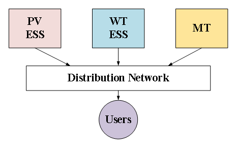
Since photovoltaic power generation and wind turbine power generation are greatly affected by external factors, causing significant fluctuations to the system, a combined power generation system with an energy storage system is used to suppress the instability of DG (Distributed Generation), as illustrated in Figure 1, to form a stable island operation.
\[\label{e7} {P_t} = {P_{\text{DG}}}(t) + {P_{\text{ESS}}}(t), \tag{7}\] where \({P_t}\) is the output of the joint energy storage device at the current moment, \({P_{DG}}(t)\) is the output value of the distributed power supply at the current moment, and \({P_{\text{ESS}}}(t)\) is the output value of the energy storage device at the current moment. See Figure 1.
The load is classified into three levels based on user importance: first-level, second-level, and third-level. After a power supply network failure, the first-level load recovery power supply level is optimal. During recovery, first-level loads that cause significant harm in the event of a power outage are prioritized. The load priority recovery coefficient is calculated by assigning weight coefficients, establishing the load priority recovery set \({C_{load}}\):
\[\label{e8} {C_{i,t}} = {w_{i,t}}{P_{i,t}}{T_{i,t}}, \tag{8}\] where \({w}\) is the load level, \({P}\) is the load active power for the time period, and \({T}\) is the importance coefficient of the load type of this node at the current moment. The first-level load is always set to 10, while second- and third-level loads are weighted based on commercial and residential loads, adjusted for different times of the day.
The load on the user side is divided into controllable and uncontrollable loads. The uncontrollable load refers to fixed loads in the power system, which usually do not participate in demand response adjustments. Controllable loads refer to user-side loads adjusted based on time-of-use electricity pricing, achieved through agreements between the power company and users. During peak periods or emergencies, users actively reduce or interrupt loads per the agreement. The interruptible load model is:
\[\label{e9} P_{L,t}^{in} = (1 – {\mu _{L,t}})P_{L,t,\max }^{in}, \tag{9}\] where \({P_{L,t,\max }^{in}}\) is the maximum power of the interruptible load, and \({\mu _{L,t}} = 1\) indicates that the user load can be interrupted.
Transferable loads, which can flexibly shift between specified time periods, allow peak shaving and valley filling. Transferable load is defined such that the total load remains unchanged over a period, even during fault recovery:
\[\label{e10} P_{L,t}^{ch} = \eta P_{L,t,\max }^{ch}, \tag{10}\] where \({P_{L,t,\max }^{ch}}\) is the maximum power of the transferable load, and \({\eta}\) is the transferable load factor. To minimize energy waste due to wind and light curtailment, controllable load adjustments aim to align the load curve with the joint energy storage output curve, reducing deviations and achieving effective distributed energy resource utilization. Variance is used to measure the deviation:
\[\label{e11} k = \frac{1}{{24}}\sum\limits_{t = 1}^{24} {{{({P_{L,t}} – {P_t})}^2}}, \tag{11}\] where \({P_{L,t}}\) is the controllable load power size, and \({P_t}\) is the fan output size at the current moment. During fault recovery, transfer and interrupt loads ensure controlled nodes meet wind turbine output, minimizing \({k}\).
The division principles are as follows:
1. The island should operate safely and stably, with the ability to merge into the main network.
2. The DG capacity in the island must exceed the total load, maximizing node inclusion within the island.
3. Nodes with higher load levels are prioritized during islanding.
4. If the energy storage capacity cannot meet load demands, load-shedding is performed. If constraints remain unsatisfied, the island is re-divided.
5. To avoid adverse effects from DG off-grid, the number of islands is minimized.
The actual output value of DG at the fault moment is used as the power source for all island nodes, aiming to restore the maximum power loss of important nodes:
\[\label{e12} f = \max \sum\limits_{i \in {N_k}} {{x_i}{\lambda _i}{P_{Li}}}, \tag{12}\] where \({\lambda _i}\) represents the load level weight: 100 for first-level, 10 for second-level, and 1 for third-level loads. \({x_i}\) is the switching state, where 0 indicates disconnection, and 1 indicates connection.
The constraints include:
Power flow constraints: \[\label{e13} \begin{cases} \Delta P = {P_{Gi}} – {V_i}\sum\limits_{j \in i} {{V_j}({G_{ij}}\cos {\theta _{ij}} – {B_{ij}}\sin {\theta _{ij}})}, \\ \Delta Q = {Q_{Gi}} – {V_i}\sum\limits_{j \in i} {{V_j}({G_{ij}}\sin {\theta _{ij}} – {B_{ij}}\cos {\theta _{ij}})} . \end{cases} \tag{13}\]
Branch maximum capacity constraint: \[\label{e14} {({P_{l,t}})^2} + {({Q_{l,t}})^2} \le {(S_{l,t}^{\max })^2}. \tag{14}\]
Voltage constraints: \[\label{e15} {V_{i,\min }} \le {V_{i,t}} \le {V_{i,\max }}. \tag{15}\]
Topology constraints: \[\label{e16} {B_i} \in G , \tag{16}\] where \({B_i}\) is the network topology for the island, and \(G\) is the topological set of radial networks meeting the requirements.
Eq. (13) is the power flow constraint in the line, where \(i\) and \(j\) represent the starting and ending nodes of the branch, respectively. Eq. (14) represents the maximum capacity constraint of the branch, where \(P\), \(Q\), and \(S\) are the active power, reactive power, and apparent power, respectively. Eq. (15) defines the voltage constraint, where \({{V_{i,t}}}\) is the voltage value of node \(i\) during the \(t\)-period, and \({V_{i,\min }}\) and \({V_{i,\max }}\) are the lower and upper voltage limits of node \(i\), respectively. In Eq. (16), \({{B_i}}\) denotes the network topology of the island, and \(G\) represents the topological set of all radial networks in the distribution network meeting the requirements.
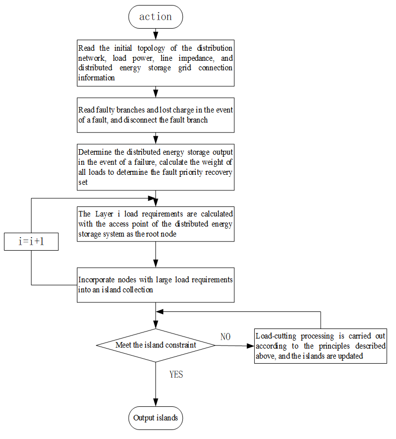
1. **Initial Traversal:** Begin by searching all paths connected to the node associated with the distributed power supply as the starting point. The nodes directly connected to this starting point are classified as the first layer, while the nodes directly connected to the first layer form the second layer, and so on. Calculate the total load for each layer node to form a load recovery set \({{C_{i,t}}}\), and arrange it from largest to smallest.
2. **Node Analysis:** Compare the \({{C_{i,t}}}\) values of the first-layer nodes, store the node with the largest value in the island set, and analyze the next-layer nodes. Calculate the power of the two-layer nodes and replace the nodes in the original island set with the larger value. Continue analyzing each layer node sequentially until the island power requirements are not satisfied. Output the division plan for this island.
3. **Important Node Inclusion:** Check if all important nodes in the load priority recovery set are included in the island. If any isolated important load nodes remain, include them in the nearest island by performing a power radius search on the formed islands.
4. **Power Constraint Validation:** Check for power overrun issues. If power constraint requirements are not met, prioritize the removal of interruptible loads according to the demand response characteristics of the load. Then, reduce the transferable load until the power constraint is satisfied. Finally, output the islanding scheme. The specific process is shown in Figure 2.
When a fault occurs, the faulty branch will be disconnected immediately. Subsequently, the islanding method described in Part 2 is used to restore power to critical loads. The remaining non-faulty power loss areas and operable switch groups are then calculated, and the main network is reconstructed to supply power to the remaining unrecovered areas.
The network reconstruction of the distribution network aims to restore the power supply to non-fault areas and minimize network losses. The objective function is formulated as follows:
\[\label{e17} f\min = {\rho _1}\left(\sum\limits_{d \in F} {(1 – {k_d}) + \sum\limits_{d \in L} {{k_d}} } \right) + {\rho _2}\sum\limits_{i \in N} {\frac{{P_i^2 + Q_i^2}}{{U_i^2}}} {R_i} + {\rho _3}\sum\limits_{i \in N} {{x_i}{\lambda _i}{P_{Li}}}. \tag{17}\]
In the formula, \({\rho _1}\), \({\rho _2}\), and \({\rho _3}\) are the weights of the three objectives and are usually valued according to the actual situation of fault recovery; \({{k_d}}\) indicates the state of the switch, where 1 denotes closure and 0 denotes disconnection. \(L\) and \(F\) represent the sets of contact switches and segment switches, respectively; \({P_i^2}\), \({Q_i^2}\), \({U_i^2}\), and \({R_i}\) are the active power, reactive power, voltage, and impedance at node \(i\), respectively.
The constraints follow the same formulations as Eqs. (13) – (16).
The Whale Optimization Algorithm (WOA) is an intelligent algorithm that simulates whales’ food-searching behavior in the ocean to find the optimal solution. Each whale’s position represents a feasible solution. The predation process includes three steps: surrounding the prey, rotating to update the position, and attacking the bubble net. The whale’s position is updated as follows:
\[\label{e18} D = \left| {C \times {X^ * } – X(t)} \right| , \tag{18}\]
\[\label{e19} X(t + 1) = {X^ * }(t) – A \times D, \tag{19}\]
\[\label{e20} A = 2ar – a , \tag{20}\]
\[\label{e21} C = 2r , \tag{21}\]
\[\label{e22} a = 2 – 2t/T . \tag{22}\]
In these equations, \(A\) and \(C\) are vector coefficients, where \(A > 1\) indicates the surrounding prey stage. \(D\) represents the distance between an individual whale and the prey, \({X(t)}\) is the position of the individual whale at iteration \(t\), and \({X^ * }(t)\) is the position of the optimal individual whale at the current moment. \(r\) is a random value in [0,1], \(T\) is the maximum number of iterations, and \(t\) is the current iteration. As the number of iterations increases, the value of \(a\) decreases, resulting in \(A\) decreasing. When \(A \leq 1\), the whale enters the encirclement predation stage, updating its position spirally around the prey using Eq. (23):
\[\label{e23} x(t + 1) = d{e^{bl}}\cos (2\pi l) + {X^ * }(t), \tag{23}\] where \(b\) is a constant in the spiral equation, and \(l\) is a random value in (-1,1).
The spitting bubble attack and spiral position update are specific hunting behaviors of whales. These behaviors are conducted simultaneously, with a selection probability \(p\), described by Eq. (24). As iterations progress, the value of \(\left| A \right|\) gradually decreases, and when it decreases to 0, the whale algorithm finds the ideal optimal solution.
\[\label{e24} X(t + 1) = \left\{ \begin{array}{l} X(t) – AD, \quad p{\rm{ < }}0.5\\ d{e^{bl}}\cos (2\pi l) + {X^ * }(t), \quad p \geq 0.5 \end{array} \right. \tag{24}\]
Initial Population Optimization
The initial population of WOA is randomly generated within a specified search space, and the initial whale position significantly affects the final iteration results. To obtain a more diverse initial population, Sobol sequences are used to generate a more uniform initial population that covers the search space comprehensively. Comparing the overall size of the population generated by random distribution and using Sobol sequence to generate 500 initial values, it is evident that the initial values generated by Sobol sequence cover the search space more completely and uniformly.
Adaptive Convergence Factor
In the whale search algorithm, the \(A\) value controls the global search ability and local development ability of the whale. When the whale population has \(A>1\), it is in the global search state, and for \(A \leq 1\), it is in the local exploration state. The size of the \(A\) value is controlled by the convergence factor \(a\). As the number of iterations increases, \(A\) decreases linearly, resulting in slow convergence in the later stages of predation. To improve the local convergence ability of the whale population in the later stages of predation, an adaptive convergence factor is proposed, as shown in Eq. (25). Using this factor, the early \(A\) value of the algorithm can be larger, and the decrease speed is slower to obtain better global search ability. In the later stage of the algorithm, the \(A\) value decreases slowly, improving the convergence accuracy.
\[\label{e25} a = 2 – 2\sin \left(\mu \frac{t}{T}\pi + \varphi \right). \tag{25}\]
Adaptive Weight Strategy
As the algorithm iterates, the formula for updating the position of whales does not change accordingly, which may cause whales to deviate from their prey in the later stages of predation and fall into local optimization. Therefore, an adaptive weight is proposed to update the position of whales. Using adaptive weights to improve the position of the whale in Eq. (19), Eq. (27) is obtained to replace the original position update formula.
\[\label{e26} \omega = 1 – \frac{{{e^{\frac{t}{T}}} – 1}}{{e – 1}}, \tag{26}\]
\[\label{e27} X(t + 1) = \omega {X^ * }(t) – A \times D. \tag{27}\]
The specific steps are as follows:
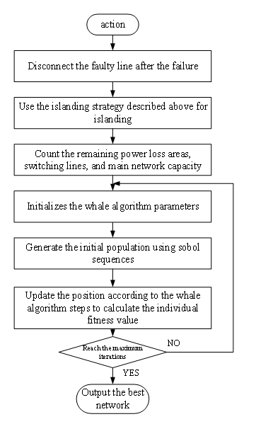
When the distribution network fails, disconnect the branch road where the fault point is located, perform island division according to the rules of the first section, and use the energy storage system to supply power to the load with higher priority.
Separate the islands from the main network to count the remaining node contact switches and segmentation switches.
Use the Sobol sequence to generate a uniform initial population, and calculate the fitness function based on the position of the initial population.
Calculate the distance between the whale and the prey using Eq. (18), and use Eq. (25) to calculate the vector coefficient instead of the original convergence factor. Update the whale position using Eq. (26) and Eq. (27).
Follow Eq. (24) to select the position update stage until the maximum number of iterations is reached.
The overall failure recovery process based on island division and the improved whale optimization algorithm is shown in Figure 3.
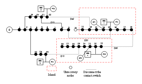
The improved IEEE33 node distribution network model is used for verification. This distribution network model consists of 33 nodes and 37 branches, with 5 contact branches numbered 33-37. The reference voltage is 12.66 kV, and the total loads of the system are \((3802.19+j2694.6)\) kVA. The structure of this distribution network is shown in Figure 4, and the specific parameters are referenced from the literature.

Distributed power generation and energy storage devices are connected at nodes 14, 15, 22, 25, 31, and 32. The load level and load type settings of each node in the system are shown in Tables 1 and 2.
| Load Level | Node Number | Load Weights |
| First | 4, 6, 15, 22, 25, 32 | 100 |
| Second | 7, 11, 14, 21, 26, 30 | 10 |
| Third | Others | 1 |
| Load Type | Node Number |
| Controllable Load | 2, 5, 9, 10, 12, 16, 14, 28, 30 |
| Uncontrollable Load | Others |
| Commercial Load | 1, 2, 5, 12, 13, 16, 17, 18, 20, 21 |
| Resident Load | 3, 7, 8, 9, 11, 14, 26, 27, 28, 29, 30, 31, 33 |
Suppose that faults occur at branches 7-26 and 9-10 at 10:00 and 22:00, respectively. The total fault duration is set to 2 hours. The specific outputs of the distributed energy storage system during the fault periods are shown in Table 3. The fault points are isolated immediately, and the fault branches are disconnected. At this time, the areas experiencing power loss due to the fault include nodes 13-18 and 26-33. The priority recovery coefficients for these lost nodes are calculated based on the load importance. Using the island division principle described earlier, distributed power generation is used to supply power to the islands. The faulted branches and islands are separated from the main network, and the remaining areas are reconstructed using the improved whale algorithm. The specific parameters of the whale algorithm are set as follows: the maximum number of iterations is 100, and the initial population size is 30.
| Distributed Appliance Number | Access Location | 10:00 Fault Output (kW) | 22:00 Fault Output (kW) |
| WT/ESS1 | 15 | 400 | 600 |
| WT/ESS2 | 22 | 250 | 420 |
| PV/ESS1 | 25 | 1000 | 0 |
| PV/ESS2 | 32 | 150 | 0 |
| MT1 | 14 | 200 | 200 |
| MT2 | 31 | 400 | 1200 |
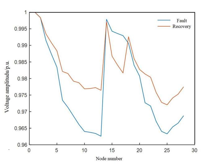
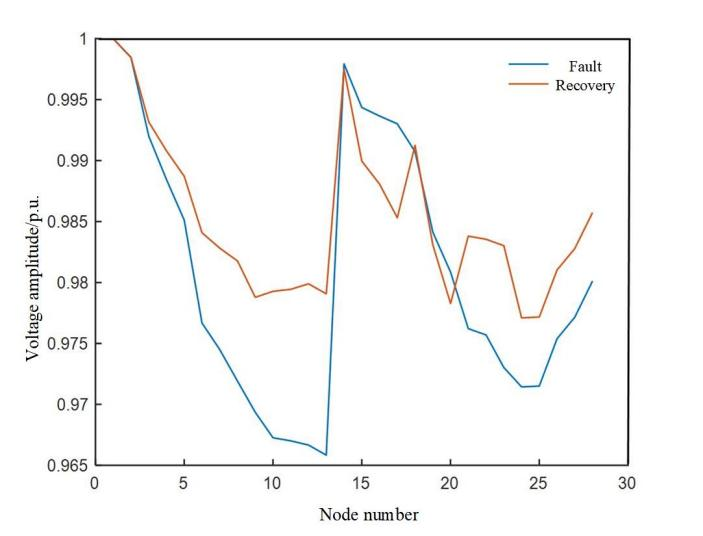
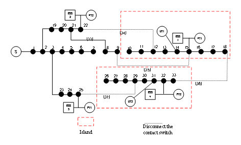
The fault recovery results are shown in Table 4, and the restored network topologies are depicted in Figures 5 and 6. The voltages of nodes before and after the fault are shown in Figures 7 and 8.
| Island Number | Load Nodes in the Island | 10:00 | 22:00 | Total Load (kW) | 10:00 | Disconnect Switch |
| 1 | 13,14,15,16,17,18 | 360 | 480 | 12-13 | 9-10 | |
| 2 | 10,11,12,22 | 210 |
|
21-22,9-10 | ||
| 4 | 26-33 | 800 | 800 | 7-26 | 7-26 |
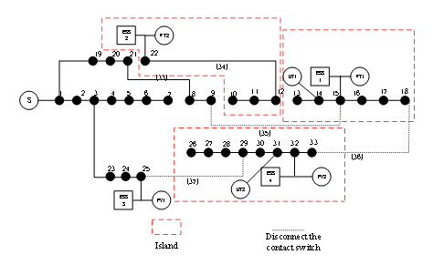
According to the analysis, fault recovery strategies differ based on the output of the distributed energy storage system and load characteristics at different times. At 10:00, the wind storage system output is small, and island 1 restores power supply to nodes 13-18. Since residential electricity demand is low and node 12 is controllable commercial electricity, it is temporarily excluded from the island. Using network reconstruction results, switch 34 is closed, and wind storage system 2 restores power to nodes 10-12. Nodes 26-33 form an island powered by the optical storage system and micro-gas turbine.
At 22:00, with increased residential electricity demand and larger wind storage system output, the photovoltaic storage system output is 0. Wind storage system 1 restores power to nodes 10-18, while micro-gas turbines support the island formed by nodes 26-33. This approach demonstrates the adaptability of the fault recovery strategy at different times, with varying network losses and voltage amplitudes after recovery (Table 5).
| Time | Fault | Recovery | Loss (kW) | Voltage Amplitude (p.u.) |
| 10:00 | 83.239 | 60.499 | 0.9612 | 0.9747 |
| 22:00 | 133.568 | 104.747 | 0.9572 | 0.9783 |
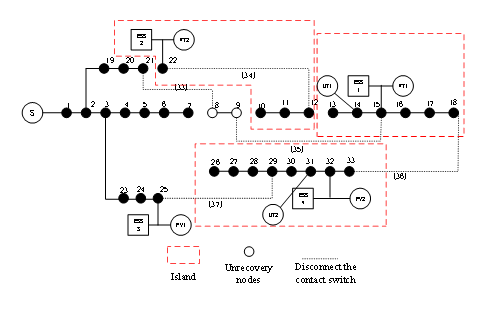
To further verify the effectiveness of the proposed recovery strategy, three cases were compared, as shown in Table 6:
Case 1: Only island division is used to restore the lost power area without network reconstruction.
Case 2: The load characteristics and demand response are not considered, only the load level is used for recovery.
Case 3: The proposed strategy in this paper.
| Case | Lost Power Load Node | Mainnet Load Recovery (kW) | Island Load Recovery (kW) | Loss (kW) | Switching Actions |
| 1 | 8,9 | 2000 | 1565 | 141.463 | 2 |
| 2 | 10 | 2210 | 1460 | 102.348 | 2 |
| 3 | Empty | 2120 | 1565 | 60.499 | 4 |
As shown in Figures 9 and 10, Case 3, using the proposed strategy, yields optimal results compared to the other cases. It ensures maximal utilization of the distributed energy storage system and achieves the best recovery outcomes.
The effectiveness of the proposed improved whale algorithm (IWOA) is further verified by comparing it with PSO and traditional WOA under the same parameter settings. The results, shown in Table 7, demonstrate that IWOA achieves superior network loss reduction and faster solution times.
| Algorithm | Loss (kW) | Avg. Iterations | Solution Time (s) |
| PSO | 141.83 | 29 | 13.88 |
| WOA | 140.29 | 25 | 12.85 |
| IWOA | 139.55 | 13 | 8.27 |
In this paper, the fault recovery of the distribution network containing the distributed energy storage system is studied, and the fault recovery mode combined with the island division and the reconstruction of the distribution network is proposed, The distribution network model with the distributed energy storage system is constructed, the load demand response on the user side is taken into account when the islanding is divided, and the load cutting action is completed through the transfer and interruption of the controllable load, so that the load with high priority level can quickly restore power supply.
This work is supported by Natural Science Foundation of Hubei Province, No: 2020CFB248.