
Suppose \(\mathcal{F}\) is a family of graphs. We say that a graph \(G\) is \(\mathcal{F}\)–saturated if no element of \(\mathcal{F}\) is a subgraph of \(G\), but for any edge \(e\) in the complement of \(G\), \(G+e\) contains a subgraph isomorphic to some \(F\in \mathcal{F}\). When \(\mathcal{F} = \{L\}\) is a single graph \(L\), and G satisfies the preceding conditions, then we say that \(G\) is \(L\)-saturated. The well studied Turan function \(ex(n, \mathcal{F})\) is the maximum number of edges in any \(\mathcal{F}\)-saturated graph on \(n\) vertices. A natural dual to \(ex(n, \mathcal{F})\) is the saturation function \(Sat(n, \mathcal{F})\), which is the minimum number of edges in any \(\mathcal{F}\)-saturated graph on \(n\) vertices. We write \(Sat(n, L)\) and \(ex(n, L)\) for these two functions when \(\mathcal{F} = \{L\}\); that is, when \(\mathcal{F}\) consists of the single graph \(L\). The best known upper bound on \(Sat(n, \mathcal{F})\) for an arbitrary family \(\mathcal{F}\) is given in [27].
A natural first case to study for the saturation function is \(Sat(n, K_{r})\), where \(K_{r}\) is the complete graph on \(r\) vertices. It was shown in [39] and later independently in [15] that \(Sat(n, K_{r}) = (r-2)(n-r+2) + \binom{r-2}{2} = \binom{n}{2} – \binom{n-r+2}{2}\), and that the upper bound is uniquely realized by the join \(K_{r-2} + \overline{K}_{n-r+2}\); that is, the disjoint union of \(K_{r-2}\) with a set of \(n-r+2\) independent points, together with all \((r-2)(n-r+2)\) possible edges joining the set of independent points with the vertices of the \(K_{r-2}\). At the opposite extreme in edge density from \(K_{r}\) for connected graphs is the star \(K_{1,t}\), where there is the following result.
If \(n\geq t + \lfloor \frac{t}{2} \rfloor\), then \(Sat(n, K_{1,t}) = \big{(}\frac{t-1}{2}\big{)}n – \frac{1}{2}\lfloor \frac{t^{2}}{4}\rfloor.\)
\(t+1\le n < t + \lfloor \frac{t}{2} \rfloor\), then \(Sat(n, K_{1,t}) = \binom{t}{2} + \binom{n-t}{2}\).
Let \(H\) be a fixed graph (and we think of \(H\) as the “host”), and \(L\) a given graph (where we think of \(L\) as the “forbidden” graph). A subgraph \(G\) of \(H\) is called \(L\)–saturated in \(H\) (or just \(L\)–saturated if \(H\) is understood) if \(L\) is not a subgraph of \(G\), but for any edge \(e\in E(H) – E(G)\) the graph \(G + e\) contains the subgraph \(L\). We then let \(ex(H, L)\) and \(Sat(H, L)\) be the maximum and minimum (respectively) number of edges in a graph \(G\) which is \(L\)-saturated in \(H\). If \(L\) is not a subgraph of \(H\) then we let \(Sat(H, L) = ex(H, L) = |E(H)|\). Observe also that \(Sat(n, L) = Sat(K_{n}, L)\) and \(ex(n, L) = ex(K_{n}, L)\).
This saturation problem for general host graphs \(H\) was to our knowledge first mentioned in [15]. Erdos examined \(Sat(H, K_{3})\) in [13]. In [15] the value of \(Sat(K_{r,s}, K_{m,n})\), \(m\le r\) and \(n\le s\), was conjectured, where we specify that the \(m\)-set (resp. \(n\)-set) of the \(K_{m,n}\) occur in the \(r\)-set (resp. \(s\)-set) of the \(K_{r,s}\). The conjecture was confirmed independently by Bollobás [6], [3], and Wessel [], [37], where they showed that \(Sat(K_{r,s}, K_{m,n}) = rs – (r – m + 1)(s – n +1)\). Let \(Sat'(K_{r,s}, K_{m,n})\) be the saturation function for the unordered version of this problem; that is, where we allow the \(m\)-set of \(K_{m,n}\) to be either in the \(r\)-set or the \(s\)-set of \(K_{r,s}\), and the \(n\)-set is in the opposite set of \(K_{r,s}\). In [33] it was conjectured that \(Sat'(K_{r,r}, K_{m,n}) = (m + n – 2)r – \lfloor \big{(}\frac{m+n-2}{2}\big{)}^{2} \rfloor\). In [20] it was shown that \(Sat'(K_{r,r}, K_{m,n})\geq (m + n – 2)r – (m + n – s)^{2}\) and that the conjecture holds in the case \(m = 2\) and \(n = 3\).
Another host graph that has been considered is the complete multipartite graph. The above saturation results for bipartite hosts were generalized to \(k\)-uniform multipartite hypergraph hosts by Alon [2]. In this paper he proves a result on extremal sets using methods of multilinear algebra, and from this derives results on saturation in multipartite hypergraphs. The bipartite host results were also generalized by Pikhurko in his Ph.D. thesis at Cambridge [34]. Now let \(K_{k}^{n}\) be the complete multipartite graph on \(k\) partite sets, each of size \(n\). In [18] the values of \(Sat(K_{k}^{n}, K_{3})\) were determined for all \(k\geq 4\) for large enough \(n\), and also determined for \(Sat(K_{3}^{n}, K_{3})\) for all \(n\).
For any graph \(G\), let \(S(G)\) denote the set of all graphs that can be obtained from \(G\) by inserting any number of points of degree 2 along any set of edges of \(G\), and we call any such graph a subdivision of \(G\). Some also call this set of graphs \(T(G)\), and any member of \(T(G)\) a topological \(G\). Slightly abusing notation and for brevity, we sometimes refer to an arbitrary member of \(S(G)\) as an \(S(G)\) or just by the symbol \(S(G)\).
There has been substantial research concerning subdivisions of graphs in the context of both the saturation function \(Sat(n,L)\) and the Turan function \(ex(n,L)\). A direct influence on our work here was the paper [17], which we discuss below. In [29] the set of possible values \(|E(H)|\) for \(C_{k}\)-saturated saturated graphs \(H\) (where \(C_{k}\) is the cycle on \(k\) points) was determined. Next we mention results related to the Turan number for subdivision families. In [5] the authors investigate \(ex(n,S(F))\), where \(F\) is obtained from a cycle by joining a point on the cycle with edges only to points off the cycle, or only to points on the cycle, and again \(S(F)\) is the family of all subdivisions of such an \(F\). We mention also the deep papers [24], [23], and [12], among others, exploring \(ex(n,S(F))\) where \(F\) is the complete bipartite graph in some cases. One of the goals in this research is to find, for a given graph \(G\) the exponent \(r, \; 1 < r < 2,\) for which \(ex(n, G) = \Theta(n^{r})\). Another goal is to show that for any such \(r\) there is a graph \(G\) for which \(ex(n, G) = \Theta(n^{r})\).
Moving closer to “gridlike” graphs, we mention work on saturation in the hypercube, denoting by \(Q_{n}\) the hypercube of dimension \(n\). In [11] it was shown that \(Sat(Q_{n}, Q_{2})\le (\frac{1}{4} + o(1))|E(Q_{n})|\), and conjectured that this bound was best possible. In [25] this conjecture was disproved, where it was shown that for every fixed \(m\), there exists a \(Q_{m}\)-saturated subgraph of \(Q_{n}\) with \(o(|E(Q_{n}))\) edges. They also improved on the earlier bound on \(Sat(Q_{n}, Q_{2})\) by showing that \(Sat(Q_{n}, Q_{2}) < 10\cdot 2^{n}\) and asked for which \(m\) is it true that \(Sat(Q_{n}, Q_{m}) = O(2^{n})\). It was shown in [32] that this holds for every \(m\geq 2\), specifically, that \(Sat(Q_{n}, Q_{m})\le (1+o(1))72m^{2}2^{n}\).
In a related paper [31] to this one, the authors considered as a host the multidimensional grid \(P_{m}^{r} = P_{m}\times P_{m}\times \cdots \times P_{m}\); that is, the \(r\)-fold cartesian product of paths \(P_{m}\) on \(m\) points as the host graph, where the guest graph is the star \(K_{1,t}\). In that paper the following results for the function \(Sat(P_{m}^{r}, K_{1,t})\) were proved.
\(Sat(P_{m}^{2}, K_{1,3}) = \frac{2}{3}m^{2} + O(m).\)
\(Sat(P_{m}^{2}, K_{1,4}) = \frac{6}{5}m^{2} + O(m).\)
2. In dimension \(r\geq 3\):
\(Sat(P_{m}^{r}, K_{1,2}) = \frac{1}{3}m^{r} + O(m^{r-1}).\) (This result for \(r=2\) was implicit in results of [28].)
For \(t\geq 4\) and \(t\) even, \(Sat(P_{m}^{r}, K_{1,t})\le m^{r}\big{(}\frac{t}{2} – \frac{4}{5}\big{)} + Ktm^{r-1}\), where \(K\) is a constant.
For \(t\geq 3\) and \(t\) odd, \(Sat(P_{m}^{r}, K_{1,t})\le m^{r}\big{(}\frac{t}{2} – \frac{5}{6}\big{)} + Ctm^{r-1}\), where \(C\) is a constant.
\(Sat(P_{m}^{r}, K_{1,t}) \geq rm^{r}\big{(}\frac{t-1}{4r-t+1}\big{)} – rm^{r-1}.\) (This also holds for \(r = 2\).)
In this paper we continue the study of saturation in the host \(P_{m}^{r}\). Let \(S(K_{4})\) be the family of all graphs which are subdivisions of \(K_{4}\). In this paper we obtain results on \(Sat(P_{m}^{r}, S(K_{4}))\). Definitions and the precise statement of results follow in the next subsection.
It is useful to mention the connection of the saturation function \(Sat(G, H)\) to applications in the area of bootstrap percolation, where we have drawn on [8] and [30] for the overview which follows. In that area the general idea is to analyze diffusion or infection processes which spread through the vertices or edges of a graph. As such, this models in this area are useful in describing magnetic materials, fluid flow in rocks, computer storage systems, and spreading of rumors. So this area has been of interest to physicists, computer scientists, and sociologists; see [1] and [35].
In the vertex version, we begin with a starter set of vertices \(A_{0}\subseteq V(G)\) in some graph \(G\), and then build a sequence of sets \(A_{t}\subseteq V(G)\), \(t\geq 0\), where \(A_{t}\supseteq A_{t-1}\) for \(t\geq 1\), according to some rule. Letting \(\langle A_{0} \rangle = \cup_{t\geq 0} A_{t}\), one question of interest is whether \(\langle A_{0} \rangle = V(G)\); that is, whether the process diffuses to all vertices in \(G\). In this case we say that \(A_{0}\) percolates \(G\), or that \(A_{0}\) is a percolating set for \(G\).
A popular model of bootstrap percolation is \(r\)–neighbor bootstrap percolation, where the diffusion process is given by \(A_{t+1} = A_{t}\cup \{v\in V(G): |N(v)\cap A_{t}| \geq r\}\). Thus a vertex joins set \(A_{t+1}\) if at least \(r\) of its neighbors are already in \(A_{t}\); that is these neighbors have already been infected by time \(t\). One may choose \(A_{0}\) randomly (see [9]); that is, each vertex is initially infected with probability \(p\) independently of all other vertices. We then consider the event \(\langle A_{0} \rangle = V(G)\), and define the critical percolation probability by
\[p_{c}(G,r) = inf \left\{ p: Prob_{p}[ \langle A_{0} \rangle = V(G)] \geq \frac{1}{2} \right\},\]
The class of \(d\)-dimensional grids \(P_{m}^{d}\) is of interest as a possible graph \(G\) for this work. Among the results here we mention the work of Holroyd [22] who proved \(p_{c}(P_{m}^{2}, 2) = \dfrac{\pi^{2}}{18\;log(n)} + o\left(\dfrac{1}{log(n)}\right)\). Holroyd introduced a function \(\lambda(d,r)\) (which we omit here), which was used by Balogh [4] in proving the sharp threshold for all dimensions \(d\) given by
\[p_{c}(P_{m}^{d}, r) = \Big{(} \dfrac{\lambda(d,r) + o(1)}{log_{r-1}(n)}\Big{)}^{d-r+1},\] where \(log_{r-1}(n)\) is the \((r-1)\)-times iterated logarithm.
Another model considers a diffusion process through edges called \(H\)–bootstrap percolation. As notation, for any set \(S\) of edges in some graph \(G\), let \([S]\) denote the subgraph of of \(G\) induced by \(S\). Now let \(G\) and \(H\) be graphs, and \(E_{0}\subseteq E(G)\) such that \(H\) is not a subgraph of \([E_{0}]\). We say that \(E_{0}\) is weakly \(H\)-saturated in \(G\) if there is an ordering \(e_{1}, e_{2}, \cdots , e_{k}\) of the edges in \(E(G) – E_{0}\) such that for the edge sets \(E_{1} = E_{0}\cup \{e_{1}\}\), and generally \(E_{i} = E_{i-1}\cup \{e_{i}\}\), \(1\le i\le k\), the following holds. For each \(i\geq 1\) there is a subgraph \(H' \cong H\) contained in \(E_{i}\), but \(H'\) not contained in \(E_{i-1}\). That is, the addition of edge \(e_{i}\) creates a copy of \(H\) in \(E_{i}\) not present in \(E_{i-1}\). The research problem, proposed by Bollobás in [7], is then to find a minimum size weakly \(H\)-saturated set in \(G\), denoted by \(wsat(G,H)\).
In an equivalent model for \(H\)-bootstrap percolation, starting again with some \(E_{0}\subseteq E(G)\), we build a sequence \(E_{0}\subset E_{1}\subset E_{2} \cdots\) of edge sets \(E_{i}\subseteq E(G)\) of \(G\) according to the following rule:
\[E_{t+1} = \{e\in E(G)-E_{t}:\exists H' \cong H\;\, \text{with}\;\; H' \subseteq [E_t \cup \{e\}]\;\; \text{and} \;\; H' \nsubseteq [E_t]\}.\]
If \(E_{k} = E(G)\) for some \(k\geq 0\), then we say that our “starter” set \(E_{0}\) is an \(H\)-percolating set in \(G\). Here we add entire sets of edges to our percolating process at a time. Note that for any \(E'\subseteq E(G)\) we have that \(E'\) is weakly \(H\)-saturated in \(G\) if and only if \(E'\) is \(H\)-percolating in \(G\). Clearly the minimum size of an \(H\)-percolating set in \(G\) is also \(wsat(G,H)\). In this second model one can also ask for the maximum time \(t\), over all starting sets \(E_{0}\), until the percolation process stabilizes; that is until \(E_{t+1} = E_{t}\). We mention [8] and [30] among others for work on this topic.
For the connection between the saturation function \(Sat(G,H)\) studied in this paper and percolation, observe that \(wsat(G,H)\le Sat(G,H)\). As proof, take any edge set \(E'\subseteq E(G)\) realizing \(Sat(G,H)\). Then \(E'\) is in fact weakly saturated in \(G\). This is because by definition \(H\nsubseteq [E']\), and for any \(e\in E(G) – E'\) we have \(H\subseteq E'\cup \{e\}\). Thus under any ordering \(e_{i}, i\geq 1\), of the edges in \(E(G) – E'\) the sets \(E_{i}\) given by \(E_{0} = E'\), and \(E_{i} = E_{i-1} \cup \{e_{i}\}\) for \(i\geq 1\) gives a process witnessing that \(E'\) is weakly \(H\)-saturated in \(G\); that is a process for which \(E_{k} = E(G)\), where \(k = |E(G)| – |E'|\). Thus \(wsat(G,H)\le |E'| = Sat(G,H)\). Bollobás conjectured that we have equality for the \(K_{r}\)-percolation process in \(K_{n}\); that is \(wsat(K_{n},K_{r}) = Sat(K_{n},K_{r}) = \binom{n}{2} – \binom{n-r+2}{2}\), the last equality having already been mentioned in our introduction. This conjecture was verified independently in [2], [26], and [19].
Thus the upper bounds and exact results on \(Sat(P_{m}^{r}, S(K_{4}))\) provided in this paper also act as upper bounds for \(wsat(P_{m}^{r}, S(K_{4}))\); that is, for the minimum size of starter set in the \(S(K_{4})\)-bootstrap percolation on \(P_{m}^{r}\). More generally one can use upper bounds on \(Sat(G,H)\) to give upper bounds on the minimum size of a starter \(E_{0}\) which percolates \(G\) in the \(H\)-percolation process on \(G\).
Finally we mention the dynamic survey [16] which gives a broad and detailed coverage of the area of saturation in graphs and hypergraphs. Another useful survey is given by Gould in [21], among other works on saturation by this author.
We begin with some definitions, starting with the multidimensional grid \(P_{m}^{r}\) for positive integers \(r\geq 2\) and \(m\geq 3\). It has vertex set \(V(P_{m}^{r}) = \{ x = ( x_{1}, x_{2}, \cdots, x_{r} ): x_{i}\) an integer with \(1\le x_{i}\le m \}\), so vertices are \(r\)-tuples \(x\) with \(i\)’th coordinate \(x_{i}\) being an integer in \([m]\). The edge set is given by \(E(P_{m}^{r}) = \{ xy: x,y\in V(P_{m}^{r}), \; \sum_{i=1}^{r}|x_{i} – y_{i}| = 1 \}.\) So \(xy\) is an edge in \(P_{m}^{r}\) precisely when \(x\) and \(y\) disagree in exactly one coordinate, and in that coordinate they differ by \(1\). A straightforward induction shows that \(|E(P_{m}^{r})| = rm^{r} – rm^{r-1}\).
For any subgraph \(T\) of \(P_{m}^{r}\), we let \(T(i)\) be the subgraph of \(T\) induced by points of \(T\) with \(r\)’th coordinate equal to \(i\), \(1\le i\le m\). For an edge \(xy\in E(P_{m}^{r})\), we say that \(xy\) is a \(k\)-dimensional edge if \(x\) and \(y\) disagree by \(1\) in their \(k\)’th coordinates, and hence that \(x_{i} = y_{i}\) for \(i\ne k\). For a graph \(H\) and subgraph \(G\subset H\), we say that an edge \(e\in E(H) – E(G)\) is a nonedge of \(G\) in \(H\), and we let \(H[\overline{G}]\) be the subgraph of \(H\) induced by the set of nonedges of \(G\) in \(H\).
Next, given graphs \(G\) and \(H\) we let \(G\times H\), called the cartesian product of \(G\) and \(H\), be defined by \(V(G\times H) = \{ (v, w): v\in V(G), w\in V(H) \}\) and \(E(G\times H) = \{ (v_{1}, w_{1})(v_{2}, w_{2}): v_{1} = v_{2}\) and \(w_{1}w_{2}\in E(H)\), or \(w_{1} = w_{2}\) and \(v_{1}v_{2}\in E(G) \}.\) Note that \(G\times H\) can be obtained from \(G\) by replacing each vertex \(v\) of \(G\) by its own copy, call it \(H_{v}\), of \(H\), and joining two such copies \(H_{v}\) and \(H_{v'}\) by a matching joining corresponding points in these two copies precisely when \(vv'\in E(G)\). Symmetrically, \(G\times H\) can also be obtained by doing the similar replacement of vertices of \(H\) by copies of \(G\). Thus \(P_{m}^{r}\) is just the \(r\)-fold cartesian product \(P_{m}\times P_{m}\times \cdots \times P_{m}\). In our illustrations of \(P_{m}\times P_{n}\) and its subgraphs, rows are drawn from top to bottom in increasing row number. Also columns are drawn left to right in increasing column number. So point \((a,b)\in P_{m}\times P_{n}\) is in the \(a\)’th row from the top and the \(b\)’th column from the left.
We now turn to subdivisions of complete graphs as the forbidden graph for the saturation function. Clearly any member of \(S(K_{3})\) is a cycle, so \(Sat(n,S(K_{3})) = n-1\) as realized by a spanning tree of \(K_{n}\). Next, it is straightforward to show that any \(K_{4}\) minor is a member of \(S(K_{4})\) (see also Proposition 1.7.2 in [13] for a more general observation). It is also shown in [13] (Proposition 8.3.1) that any edge maximal graph without a \(K_{4}\) minor must be a \(2\)-tree, so it follows that \(ex(n, S(K_{4})) = Sat(n, S(K_{4})) = 2n-3\).
An exact result for \(Sat(n, S(K_{5}))\) and upper bounds for \(Sat(n, S(K_{t})), t\geq 6\) were given in the following result. This result motivated our work on \(Sat(P_{m}^{r}, S(K_{4}))\) which follows that result:
\(Sat(n, S(K_{5})) = \lceil \frac{3n+4}{2} \rceil\).
Let \(t\) be an integer, and \(n = d(t-1) + r\) for \(d\geq 2\) and \(0\le r\le t-2\).
If \(t\geq 5\) is odd, then \(Sat(n, S(K_{t})) \le d\big(\frac{t-1}{2}\big) + \frac{t-1}{2} + 2r = \big(\frac{t-2}{2} + o(1)\big)n\).
If \(t\geq 6\) is even, then \(Sat( n, S(K_{t})) \le d\big(\frac{t-1}{2}\big) + \frac{t}{2} + 2r-2 = \big(\frac{t-2}{2} + o(1)\big)n\).
The main results of this paper are the following.
If at least one of \(m\) or \(n\) is odd with \(m\geq 5\) and \(n\geq 5\), then \(Sat(P_{m}\times P_{n}, S(K_{4})) = mn + 1.\)
For \(m\) even and \(m\geq 4\), we have \(m^{3} + 1 \le Sat(P_{m}^{3}, S(K_{4}))\le m^{3} + 2.\)
For \(r\geq 3\) with \(m\) even and \(m\geq 4\), we have \(Sat(P_{m}^{r}, S(K_{4})) \le m^{r} + 2^{r-1} – 2\).
We use standard graph theoretic notation, as may be found for example in the texts [38] or [10]. There will be additional notation introduced when needed throughout the paper.
The following Lemma gives the lower bound for our exact result in dimension \(2\):
Proof. Let \(G\) be an \(S(K_{4})\)-saturated subgraph of \(H\). In particular \(G\) is spanning in \(H\) and contains no \(S(K_{4})\). We claim that \(G\) must be connected. Suppose not and let \(C_{1}\) and \(C_{2}\) be distinct connected components of \(G\). Since \(H\) is connected there must exist an edge \(e\in E(H) – E(G)\) having exactly one end in one (possibly in each) of \(C_{1}\) and \(C_{2}\). So \(e\) is a cut edge of \(G+e\). Since \(S(K_{4})\subseteq G + e\), this copy \(S\) of \(S(K_{4})\) must contain \(e\) since \(G\) contains no \(S(K_{4})\). Now \(e\), being a cutedge of \(G+e\) is contained in no cycle of \(G+e\), and therefore in no cycle of \(S\subset G+e\). Thus \(e\) is a cutedge of \(S\). But any \(S(K_{4})\) must be \(2-\)edge connected, contradicting \(e\) being a cut edge of this \(S = S(K_{4})\).
Thus we know that \(G\) is a connected spanning subgraph of \(H\), so \(|E(G)| \geq |V(H)| – 1\). Take any \(e\in E(H) – E(G)\). Suppose first that \(|E(G)| = |V(H)| – 1\), so that \(G\) is a spanning tree of \(H\). Then \(G+e\supseteq S(K_{4})\) and \(G\) contains only one cycle, contradicting that its \(S(K_{4})\) subgraph contains \(7\) cycles. Next suppose that \(|E(G)| = |V(H)|\), so that \(G\) is a tree plus an edge. Then \(G+e\), being a tree plus two edges, still contains fewer than \(7\) cycles, again contradicting that \(S(K_{4})\subseteq G+e\) contains \(7\) cycles. Thus \(|E(G)| \geq |V(H)|+1\), as required. ◻
We will need the following obvious remark for future reference:
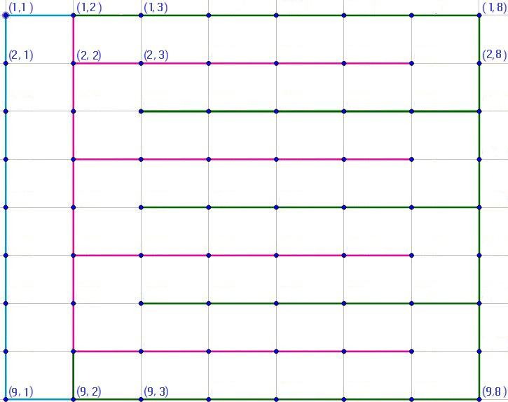
Proof. By Lemma 2.1 it suffices to prove the upper bound \(Sat(P_{m}\times P_{n}, S(K_{4})) \le mn + 1\). We will construct an \(S(K_{4})\)-saturated subgraph \(R_{m,n}\subset P_{m}\times P_{n}\) from which the upper bound follows. An example \(R_{9,8}\) is given in Figure 1.
The graph \(R_{m,n}\) may be obtained from \(P_{m}\times P_{n}\), \(m\) odd, by removing the following sets of edges:
Remove the set of edges \(\{(i,1)(i,2): 2\le i\le m-1 \}\); that is, remove the first edge of row \(i\), \(2\le i\le m-1\).
Remove the set of edges \(\{(i,m-1)(i,m): i\) even, \(2\le i\le m-1 \}\); that is, remove the last edge in each row \(i\) with \(i\) even.
Remove the set of edges \(\{(i,2)(i,3): i\) odd, \(3\le i\le m-2 \}\); that is, remove the second edge in each row \(i\) with \(i\) odd, \(3\le i\le m-2\).
Remove the set of edges \(\{(i,j)(i+1,j): 3\le j\le n-1, 1\le i\le m-1 \}\); that is, remove all edges in columns \(j\), \(3\le j\le n-1\).
We now verify that \(R_{m,n}\) is a \(S(K_{4})\)-saturated subgraph of \(P_{m}\times P_{n}\) with \(m\) odd. The reader can use Figure 1 illustrating \(R_{9,8}\) when reading the following case arguments.
First we note that \(R_{m,n}\) contains no \(S(K_{4})\), since \(R_{m,n}\) contains exactly \(3\) cycles, while an \(S(K_{4})\) contains \(7\) cycles.
It remains to show that for any nonedge \(e\in E(P_{m}\times P_{n}) – E(R_{m,n})\) of \(R_{m,n}\), \(R_{m,n}+e\) contains a cycle \(W\) and vertex \(x\notin W\) as described in Observation 2.2. As notation, when \(A\) and \(B\) are two vertices of \(R_{m,n}\) along the same row or column of \(P_{m} \times P_{n}\), we write \(A \cdots B\) to mean the path in \(P_{m} \times P_{n}\) along that row or column joining joining \(A\) and \(B\). Let \(W'\) be the length \(2m\) cycle of \(R_{m,n}\) having the vertices, listed in a traversal of \(W'\), \((1,1), (2,1) \cdots (m,1),(m,2), (m-1,2) \cdots (1,2), (1,1)\), and let \(W''\) be the length \(2m+2n-6\) cycle having the vertices \((1,2), (2,2) \cdots (m,2),(m,3) \cdots (m,n) \cdots (1,n) \cdots (1,2)\). We consider the following representative cases.
Suppose first that \(e\) is a horizontal nonedge; that is, \(e = (i,j)(i,j+1)\). Consider first the case \(e = (i,n-1)(i,n)\), \(i\) even. Then let \(W = W'\), and let \(x = (i,n)\). Then the three independent \(x-W\) paths are \(P_{1} = (i,n), (i,n-1) \cdots (i,2)\), \(P_{2} = (i,n), (i-1,n) \cdots (1,n) \cdots (1,2)\), and \(P_{3} = (i,n), (i+1,n) \cdots (m,n),(m,n-1) \cdots (m,2)\). The case \(e = (i,2)(i,3)\) for \(i\) odd is similar, using the same \(W\) and \(x = (i,n)\). The final kind of horizontal nonedge is of the form \(e = (i,1)(i,2)\), for some \(2\le i\le m-1\). Then let \(W = W''\), \(x = (i,1)\), and the three \(x-W\) paths are \(P_{1} = (i,1), (i,2)\), \(P_{2} = (i,1), (i-1,1) \cdots (1,1), (1,2)\), and \(P_{3} = (i,1), (i+1,1) \cdots (m,1), (m,2)\).
Second, suppose \(e\) is a vertical nonedge, starting with the case \(e = (i,k)(i+1,k)\), with \(i\) even, \(3\le k\le n-1\), and \(i < m-1\). Then let \(x = (i+1,n)\), \(W = W'\), and the three \(x-W\) paths are \(P_{1} = (i+1,n), (i+1,n-1) \cdots (i+1,k), (i,k), \cdots (i,2)\), \(P_{2} = (i+1,n), (i,n) \cdots (1,n), (1,n-1) \cdots (1,2)\), and \(P_{3} = (i+1,n), (i+2,n) \cdots (m,n), (m,n-1) \cdots (m,2).\) If \(i = m-1\), then take \(x = (1,2)\) and the cycle \(W = (m-1,k)(m,k)\cdots (m,2)(m-1,2)\cdots (m-1,k)\). Then we have three independent \(x-W\) paths in \(R_{m,n}+e\) given by \(P_{1} = (1,2)(1,3)\cdots (m-1,2)\), \(P_{2} = (1,2)\cdots (1,n)(2,n)\cdots (m,n)\cdots (m,k)\), and \(P_{3} = (1,2)(1,1)\cdots (m,1)(m,2)\).
The other type of vertical nonedge is \(e = (i,k)(i+1,k)\), with \(i\) is odd. Consider first the special case \(i = 1\), so \(e = (1,k)(2,k)\), \(3\le k\le n-1\). Then take the cycle \(C = (1,k), (2,k), (2,k-1), \cdots, (2,2), (1,2) \cdots, (1,k)\). Now take \(x = (m,2)\), and we have the three \(x – C\) paths \(P_{1} = (m,2), (m-1,2), \cdots, (2,2)\), \(P_{2} = (m,2), (m,1), (m-1,1), \cdots, (1,1), (1,2)\), and \(P_{3} = (m,2), (m,3),\\ \cdots, (m,n), (m-1,n), \cdots, (1,n), (1,n-1), \cdots, (1,k)\). For the general case with \(3\le i\le m-2\) (still with \(e = (i,k)(i+1,k)\), \(i\) odd) take the cycle to be \(W', x = (i,n)\), and the three \(x – W'\) paths are \(P_{1} = (i,n), \cdots, (i,k), (i+1,k), \cdots, (i+1,2)\), \(P_{2} = (i,n), \cdots, (1,n), \cdots, (1,2)\), and \(P_{3} = (i,n), \cdots, (m,n), (m,n-1), \cdots, (m,2)\). ◻
In this section we give a construction that realizes upper bounds for \(Sat(P_{m}^{3}, S(K_{4}))\), \(m\) even and \(m\geq 4\). It provides the basic intuition behind our general construction realizing upper bounds for \(Sat(P_{m}^{r}, S(K_{4}))\) for arbitrary dimension \(r\geq 4\) that we give in the next section. We refer to the four points of degree \(3\) in an \(S(K_{4})\) as junction points of that \(S(K_{4})\), and to the six internally disjoint paths in this \(S(K_{4})\) joining pairs of junction points as junction paths.
For any subset \(S\subset V(P_{m}^{u})\), \(u\geq 1\), we let \(\underline{S\ast i} \subset V(P_{m}^{u+1})\) be defined by \(S\ast i = \{(x_{1}, x_{2}, \cdots , x_{u}, i): (x_{1}, x_{2}, \cdots , x_{u})\in S \}\); that is \(S\ast i\) is obtained by appending \(i\) as the \((u+1)\)’st coordinate and leaving the first \(u\) coordinates unchanged in each point of \(S\). For example if \(S = \{(1,2,1), ( 2,3,4)\}\subset V(P_{m}^{3})\), then \(S\ast 3 = \{(1,2,1, 3), ( 2,3,4,3\}\subset V(P_{m}^{4})\). Similarly if \(T\) is a subgraph of \(P_{m}^{u}\), then \(T\ast i\) is the subgraph of \(P_{m}^{u+1}\) induced by the vertex set \(V(T)\ast i\). So clearly \(T\ast i\cong T\) under the natural isomorphism \((x_{1}, x_{2}, \cdots, x_{u})\mapsto (x_{1}, x_{2}, \cdots, x_{u}, i)\) over all \((x_{1}, x_{2}, \cdots, x_{u})\in V(T)\).
We begin by constructing a subgraph \(S_{2}\subset P_{m}^{2}\) for \(m\) even:
Let \(V(S_{2}) = V(P_{m}^{2})\)
Let \(SQ_{2}\) be the subgraph of \(P_{m}^{2}\) induced by the boundary cycle of \(P_{m}^{2}\); that is, \(SQ_{2}\) is the graph induced by the set of edges \(\{(x,j)(x,j+1): x = 1\) or \(m, 1\le j\le m-1\} \cup \{(i,y)(i+1,y): y = 1\) or \(y = m, 1\le i\le m-1\}\).
For every vertex \(v = (s,1)\in S_{2}(1)\) and \(w = (s,m)\in S_{2}(m)\), \(2\le s < m\), define the path \(D(v,2)\) by;
if \(s\) is even, then \(D(v,2) = (s,1) – (s,2) – (s,3) – \cdots – (s, m-1)\), and
if \(s\) is odd, then \(D(v,2) = (s,2) – (s,3) – (s,4) – \cdots – (s, m)\).
For \(w = (s,m)\), let \(D(w,2) = D((s,1),2)\).
Let \(D(2) = \cup_{v = (s,1), 2\le s < m} D(v,2)\)
Let \(S_{2} = SQ_{2}\cup D(2)\).
End of construction of \(S_{2}\).
Each of the two rectangles in Figure 2 consisting of straight horizontal or vertical edges is a copy of \(S_{2}\). The curved lines are used in the construction of \(S_{3}\subset P_{m}^{3}\) which follows, and can be ignored for now. Apart from the boundary of \(S_{2}\), the horizontal straight lines represent paths \(D(v,2)\). For example, (suppressing third coordinates) we have \(D((2,1), 2) = (2,1)-(2,2)\cdots – (2,m-1)\) and \(D((m-1,1), 2) = (m-1,2)-(m-1,,3)\cdots – (m-1,m)\). We will sometimes refer to \(S_{2}\) as a square. Since \(S_{2}\) is connected and contains a unique cycle (induced by its boundary), we have \(|E(S_{2})| = m^{2}\). Trivially \(S_{2}\) contains no \(S(K_{4})\) since \(S_{2}\) contains exactly one cycle, we now generalize \(S_{2}\) to obtain our construction of \(S_{3}\subset P_{m}^{3}\), an \(S(K_{4})\)-saturated subgraph of \(P_{m}^{3}\). We begin with an informal description.
\(S_{3}(1)\subset P_{m}^{3}(1)\) and \(S_{3}(m)\subset P_{m}^{3}(m)\) are defined as copies of \(S_{2}\); that is we let \(S_{3}(1) = S_{2}\ast 1\) and \(S_{3}(m) = S_{2}\ast m\). We link \(S_{3}(1)\) and \(S_{3}(m)\) by a pair of length \(m-1\) paths \(L^{3}\) and \(R^{3}\) in \(P_{m}^{3}\), where \(L^{3}\) (resp. \(R^{3}\)) is the shortest path in \(P_{m}^{3}\) joining \((1,1,1)\in S_{3}(1)\) to \((1,1,m)\in S_{3}(m)\) (resp. joining \((m,m,1)\in S_{3}(1)\) to \((m,m,m)\in S_{3}(m)\)). In fact all edges of of \(L^{3}\) and of \(R^{3}\) are 3-dimensional. Next for each \(v\in S_{3}(1)\) we will define a path \(D(v,3)\) of 3-dimensional edges such that the paths \(\{D(v,3)\}\) are vertex disjoint and each path \(D(v,3)\) is pendant on exactly one point of \(S_{3}(1)\cup S_{3}(m)\). We the let \(S_{3} = (S_{2}\ast 1)\cup (S_{2}\ast m)\cup L^{3}\cup R^{3}\cup \big{(}\{D(v,3): v\in S_{3}(1)\}\big{)}\).
The role of the paths \(\{D(v,3)\}\) is to span the gap of vertices lying between \(S_{3}(1)\) and \(S_{3}(m)\); that is, those \(v\in P_{m}^{3}\) with \(2\le v_{3}\le m-1\), in such a way as to make \(S_{3}\) a connected spanning subgraph of \(P_{m}^{3}\) while also ensuring that \(S_{3}\) is \(S(K_{4})\)-saturated. In this respect the collection of paths \(\{D(v,3)\}\) plays the role in \(S_{3}\) that was played by the set of paths \(\{D(v,2)\}\subset S_{2}\), each path \(D(v,2)\) being pendant exactly one point in \(S_{2}(1)\cup S_{2}(m)\).
Letting \(D(3) = (D(2)\ast 1)\cup (D(2)\ast m)\cup \big{(}\{D(v,3): v\in S_{3}(1)\}\big{)}\), and \(SQ_{3} = (SQ_{2}\ast 1)\cup (SQ_{2}\ast m)\cup L^{3}\cup R^{3}\), we then have the decomposition \(S_{3} = SQ_{3}\cup D(3)\), in analogy with the formula for \(S_{2}\). We may view \(SQ_{3}\) as a “skeleton” of \(S_{3}\) consisting of two cycles and attachment paths \(L^{3}\) and \(R^{3}\). The subgraph \(D(3)\) fills in the gap isolated points in \(V(P_{m}^{3}) – V(SQ_{3})\), with \(D(2)\) doing the filling using dimension 2 edges and \(\{D(v,3)\}\) using dimension 3 edges.
Let \(V(S_{3}) = V(P_{m}^{3})\)
Let the two cross sections \(S_{3}(1)\) and \(S_{3}(m)\) of \(S_{3}\) be corresponding copies of \(S_{2}\). That is, we let
\(S_{3}(1) = S_{2}\ast 1\cong S_{2}\) and \(S_{3}(m) = S_{2}\ast m\cong S_{2}\).
Define a ‘left attachment path’ \(L^{3}\) joining \((1,1,1)\) and \((1,1,m)\), and a ‘right attachment path’ \(R^{3}\) joining \((m,m,1)\) and \((m,m,m)\) by
\(L^{3} = (1,1,1) – (1,1,2) – (1,1,3) – \cdots – (1,1,m)\), and
\(R^{3} = (m,m,1) – (m,m,2) – (m,m,3) – \cdots – (m,m,m)\).
Let \(C_{1}\) (resp. \(C_{2}\)) be the unique cycle of \(S_{2}\ast 1\) (resp. \(S_{2}\ast m\)). Then let
\(SQ_{3} = C_{1}\cup C_{2}\cup L^{3}\cup R^{3}\).
(Construction of \(D(3)\)). Take the unique bipartition of \(P_{m}^{3} = A\cup B\) for which \((1,1,1)\in A\). For every vertex \(v = (a,b,1)\in S_{3}(1)\) and \(w = (c,d,m)\in S_{3}(m)\), where \(v,w\notin X(3) = \{ (1,1,1), (m,m,1), (1,1,m),\\ (m,m,m)\}\) define the paths \(D(v,3)\) and \(D(w,3)\) by;
if \(v\in A\cap S_{3}(1)\), then \(D(v,3) = (a,b,1) – (a,b,2) – (a,b,3) – \cdots – (a,b,m-1)\),
if \(v\in B\cap S_{3}(1)\), then \(D(v,3) = (a,b,2) – (a,b,3) – (a,b,4) – \cdots – (a,b,m)\).
For \(w = (c,d,m)\in S_{m}(3)\), let \(D(w,3) = D((c,d,1))\).
Recalling the subgraph \(D(2)\subset S_{2}\), let
\[D(3) = (D(2)\ast 1)\cup (D(2)\ast m) \cup \big{(} \cup_{v\in (S_{3}(1)\cup S_{3}(m))-X(3)} D(v,3)\big{)}.\]
Define sets \(\lambda(3), \rho(3), \pi_{1}(3), \pi_{2}(3)\) by
\[\begin{aligned}\lambda(3) =& \{(1,1,1), (1,1,m)\},\,\,\, \text{the set of `left attachment points' of $S_{3}$},\\ \rho(3) =& \{(m,m,1), (m,m,m)\},\,\,\, \text{the set of `right attachment points' of $S_{3}$},\\ \pi_{L}(3) =& \{L^{3}\},\,\,\, \text{the `left attachment path' of $S_{3}$, and}\\ \pi_{R}(3) =& \{R^{3}\},\,\,\, \text{the `right attachment path' of $S_{3}$}.\end{aligned}\]
Let \(S_{3} = SQ_{3}\cup D(3)\).
End of construction of \(S_{3}\).
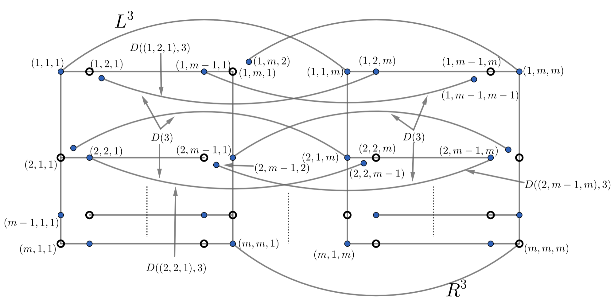
We illustrate the graph \(S_{3}\) in Figure 2.
In that Figure the two large rectangles stand for \(S_{3}(1)\) and \(S_{3}(m)\), each a copy of \(S_{2}\in P_{m}^{2}\), as described after the construction of \(S_{2}\). The straight horizontal lines represent rows in \(S_{3}(1)\) and \(S_{3}(m)\). The curved horizontal arcs represent paths \(D(v,3)\) in \(D(3)\). The darkened points at the ends of the arcs are the endpoints of such a \(D(v,3)\), and are either the pair \((i,j,2)\) and \((i,j,m)\) if \((i,j,1)\in B\), or the pair \((i,j,1)\) and \((i,j,m-1)\) if \((i,j,1)\in A\). The open circled points are those immediately preceding or following a path \(D(v,3)\) along a nonedge of dimension \(3\). For example, the path \(D((2,2,1),3)\in D(3)\) begins at the darkened point \((2,2,1)\), passes through the points \((2,2,j)\), \(1\le j\le m-1\) in order, and ends at the darkened point \((2,2,m-1)\). Then \(D((2,2,1),3)\) is followed by the open circled point \((2,2,m)\in S_{3}(m)\) joined to \((2,2,m-1)\) by a \(3\)-dimensional nonedge of \(S_{3}\) in \(P_{m}^{3}\).
We can now prove \(S(K_{4})\)-saturation for \(S_{3}\). We will say that \(H\) is a pendant subgraph in \(G\) (or of \(G\)) if \(H\) contains a cutpoint \(c\) of \(G\) such that \(H – c\) is one of the connected components of \(G – c\). Thus \(H\) is a \(c\)-component of \(G\), and in this case we will also say that \(H\) is pendant in \(G\) at \(c\).
Proof. First we show that \(S_{3}\) contains no \(S(K_{4})\), and for this suppose the contrary for contradiction. We let \(S\) be a copy of an \(S(K_{4})\) in \(S_{3}\). Let \(C_{1}\) and \(C_{2}\) be the unique cycle in \(S_{3}(1)\) and \(S_{3}(m)\) respectively.
Observe that the subgraph \([D(3)]\) of \(S_{3}\) induced by \(D(3)\) is a forest, each component of which is pendant on \(C_{1}\cup C_{2}\). Indeed, each such component \(C\) is either
a comb with base \(D(v,2)\); that is, \(C\) contains some path \(D(v,2)\), and \(C – E(D(v,2))\) is a disjoint union of paths – these paths being of the form \(D(x,3)\) for \(x\in D(v,2)\)), or
a path \(D(x,3)\) for some \(x\) in row \(1\) or row \(m\) of either \(S_{3}(1)\) or \(S_{3}(m)\).
Hence no edge of \([D(3)]\) belongs to a cycle of \(S_{3}\).
So by the above paragraph, \(S\) is a subgraph of \(H = C_{1}\cup C_{2} \cup L^{3}\cup R^{3}\). Now the \(C_{i}\) are vertex disjoint cycles, and \(L^{3}\) and \(R^{3}\) are vertex disjoint paths each having exactly one point in common with each \(C_{i}\). Therefore \(H\) contains exactly six cycles. But an \(S(K_{4})\) contains seven cycles, a contradiction.
Next we show that for any nonedge \(e = xy\) of \(S_{3}\) in \(P_{m}^{3}\), we have \(S(K_{4})\subseteq S_{3} + e\). For this, it suffices to construct a cycle \(W\subset S_{3}+e\), a point \(v\in S_{3} – V(W)\), and three \(v-W\) independent paths, in accordance with Observation 2.2.
We will need some notation. We let \(A \xrightarrow{\:\text{S} \:} B\) indicate a path from vertex \(A\) to vertex \(B\), where the symbol \(S\) refers to the path used. For example, \(S\) can be the row number of column number within either of the copies \(S_{3}(1)\) or \(S_{3}(m)\) of \(S_{2}\), or a path \(D(v,3)\), or one of the paths \(L^{3}\) or \(R^{3}\). We then indicate the concatenation of such paths by writing \(A\xrightarrow{\:\text{S} \:} B \xrightarrow{\:\text{T} \:} C \xrightarrow{\text{\: R \:}} \cdots \xrightarrow{\text{\: Q \:}} D\), resulting in a path from \(A\) to \(D\). The symbol \(A – B\) will refer to an edge in \(S_{3}+e\) joining vertices \(A\) and \(B\), and we will abbreviate \(S_{3}(1)\) (resp. \(S_{3}(m)\)) by \([1]_{3}\) (resp. \([m]_{3}\)).
The nonedge \(e = xy\) falls into one of the following categories:
\(x\) and \(y\) both belong to \(S_{3}(1)\), or \(x\) and \(y\) both belong to \(S_{3}(m)\),
\(x\in D(v,3)\) and \(y\in D(w,3)\), where \(v\) and \(w\) are at vertical or horizontal displacement \(1\) in \(P_{m}^{3}(1)\); that is, \(x = (i,j,k)\) and \(y = (i\pm 1,j,k)\), or \(x = (i,j,k)\) and \(y = (i,j\pm 1,k)\), \(2\le k\le m-1\).
\(x\in D(v,3)\) for some \(v\), and \(y\in S_{3}(1)\cup S_{3}(m)\). This possibility reduces to \(x = (i,j,m-1)\) and \(y= (i,j,m)\) for \((i,j,1)\in A\), or \(x = (i,j,1)\) and \(y= (i,j,2)\) for \((i,j,1)\in B\). That is, \(xy\) is the \(3\)-dimensional nonedge preceding or following one of the paths \(D(v,3)\).
\(x\in L^{3}\cup R^{3}\), and \(y\notin L^{3}\cup R^{3}\).
Consider first category (a). Since \(S_{3}(1)\cong S_{3}(m)\cong S_{2}\), we consider just the case \(x,y \in S_{3}(1)\). Here we pick some representative examples of such nonedges \(xy\). Consider first the subcase where \(x,y\) are in successive rows of \(S_{3}(1)\), neither row being on the boundary of \(S_{3}(1)\). So we have \(x=(i,j,1)\) and \(y=(i+1,j,1)\) with \(1< i\le m-2\). We shall first assume that \(i\) is even, so that row \(i\) is the path \((i,1,1)-(i,2,1)\cdots (i,j,m-1)\), while row \(i+1\) is the path \((i+1,2,1), (i+1,3,1)\cdots (i+1,m,1)\). Then our cycle \(W\subset S_{3} + e\) is:
\[\begin{aligned}W =& x-y \xrightarrow{\text{row $i+1$ of $[1]_{3}$}} (i+1,m,1) \xrightarrow{\text{column $m$ of $[1]_{3}$}} (1,m,1) \xrightarrow{\text{row $1$ of $[1]_{3}$}} (1,1,1)\\ &\xrightarrow{\text{column $1$ of $[1]_{3}$}} (i,1,1) \xrightarrow{\text{row $i$ of $[1]_{3}$}} (i,j,1).\end{aligned}\]
We then have the point \((m,m,1)\notin W\), together with the three independent \((m,m,1)-W\) paths in \(S_{3}+e\) given by
\[\begin{aligned}W_{1} =& (m,m,1) \xrightarrow{\text{column $m$ of $[1]_{3}$}} (i+1,m,1), (\text{ intersecting}W \text{ at }(i+1,m,1)),\\ W_{2} =& (m,m,1) \xrightarrow{\text{row $m$ of $[1]_{3}$}} (m,1,1) \xrightarrow{\text{column $1$ of $[1]_{3}$}} (i,1,1), (\text{intersecting $W$ at }(i,1,1)),\\ W_{3} =& (m,m,1) \xrightarrow{\text{$R^{3}$}} (m,m,m) \xrightarrow{\text{column $m$ of $[m]_{3}$}} (1,m,m) \xrightarrow{\text{row $1$ of $[m]_{3}$}} (1,1,m) \xrightarrow{\text{$L^{3}$}} (1,1,1),\end{aligned}\] intersecting \(W\) at \((1,1,1)\).
The construction of \(W\) and three independent \((m,m,1) – W\) paths \(W_{i}\) is very similar if \(i\) is odd, where this time the new \(W_{1}\) intersects \(W\) at \((i+1,m,1)\), the new \(W_{2}\) intersects \(W\) at \((i+1,1,1)\), while the new \(W_{3}\) is the same as the old one so has \(W\)-intersection at \((1,1,1)\).
Next consider the subcase (still in category (a)) where one of the successive rows containing \(x\) or \(y\) lies on the boundary of \(S_{3}(1)\), at first taking rows \(m-1\) and \(m\). So \(xy\) is the nonedge with \(x = (m-1,j,1)\) and \(y = (m,j,1)\), where \(2\le j\le m-1\). Since \(m-1\) is odd, row \(m-1\) of \(S_{3}(1)\) is the path \((m-1,2,1)-(m-1,3,1)\cdots -(m-1,m,1)\), while \((m-1,1,1)-(m-1,2,1)\) is a nonedge of \(S_{3}(1)\). This case is illustrated in Figure 3 where we have outlined the cycle in solid lines and three independent paths from \((1,1,1)\) to this cycle in dashed lines which are numbered. The reader may wish to use this Figure while reading the formal definition of the cycle and three paths which follow.
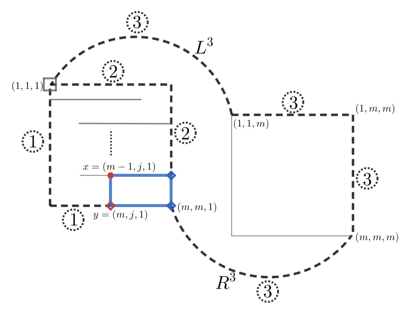
We have the cycle \(W\subset S_{3} + xy\), point \((1,1,1)\notin W\), and three independent \((1,1,1) – W\) paths as follows.
\[\begin{aligned}W =& x – y \xrightarrow{\text{row $m$ of $[1]_{3}$}} (m,m,1) – (m-1,m,1) \xrightarrow{\text{row $m-1$ of $[1]_{3}$}} (m-1,j,1) = x,\\ W_{1} =& (1,1,1) \xrightarrow{\text{column $1$ of $[1]_{3}$}} (m,1,1) \xrightarrow{\text{row $m$ of $[1]_{3}$}} (m,j,1),\\ W_{2} =& (1,1,1) \xrightarrow{\text{row $1$ of $[1]_{3}$}} (1,m,1) \xrightarrow{\text{column $m$ of $[1]_{3}$}} (m-1,m,1),\\ W_{3} =& (1,1,1) \xrightarrow{\text{$L^{3}$}} (1,1,m) \xrightarrow{\text{row $1$ of $[m]_{3}$}} (1,m,m) \xrightarrow{\text{column $m$ of $[m]_{3}$}} (m,m,m) \xrightarrow{\text{$R^{3}$}} (m,m,1).\end{aligned}\]
A very similar argument applies when the boundary row (among the two successive rows) is row \(1\). The nonedge is then \(e = (1,j,1) – (2,j,1)\) for some \(2\le j\le m-1\). The cycle \(C\) becomes \((1,1,1) – \cdots – (1,j,1) – (2,j,1) – \cdots – (2,1,1) – (1,1,1)\), and we take \(x = (m,m,1)\notin C\) together with three independent \(x-C\) analogous to the ones given in the preceding paragraph,.
We remark that the assumption \(m\) even is necessary in the preceding subcase. If \(m\) was odd, then row \(m-1\) of \(S_{3}(1)\) consists of the edges \(\{ (m-1,i,1)-(m-1,i+1,1): 1\le i\le m-2 \}\). In that case, for the nonedge \(e = (m-1,j,1) – (m,j,1), 2\le j\le m-2\) there is no \(S(K_{4})\) subgraph in \(S_{3}+e\).
To complete category (a), consider the case where \(x\) and \(y\) are in the same row of \(S_{3}(1)\). So for \(1< i< m\), \(e = xy\) is the nonedge \((i,1,1)-(i,2,1)\) if \(i\) is odd, or the nonedge \((i,m-1,1)-(i,m,1)\) if \(i\) is even. The proofs being very similar, we suppose that the nonedge is \(e = (i,1,1)-(i,2,1)\) with \(i\) odd. Then we have the cycle \(W\subset S_{3}+e\) given by
\[\begin{aligned}W = &(i,1,1)-(i,2,1) \xrightarrow{\text{row $i$ of $[1]_{3}$}} (i,m,1) \xrightarrow{\text{column $m$ of $[1]_{3}$}} (1,m,1) \xrightarrow{\text{row $1$ of $[1]_{3}$}} (1,1,1)\\ &\xrightarrow{\text{column $1$ of $[1]_{3}$}} (i,1,1).\end{aligned}\].
Taking the point \((m,m,1)\notin W\), we obtain the three independent \((m,m,1)-W\) paths
\[\begin{aligned}W_{1} =& (m,m,1) \xrightarrow{\text{column $m$ of $[1]_{3}$}} (i,m,1),\\ W_{2} =& (m,m,1) \xrightarrow{\text{row $m$ of $[1]_{3}$}} (m,1,1) \xrightarrow{\text{column $1$ of $[1]_{3}$}} (i,1,1),\\ W_{3} =& (m,m,1) \xrightarrow{\text{$R^{3}$}} (m,m,m) \xrightarrow{\text{column $m$ of $[m]_{3}$}} (1,m,m) \xrightarrow{\text{row $1$ of $[m]_{3}$}} (1,1,m) \xrightarrow{\text{$L^{3}$}} (1,1,1).\end{aligned}\]
Consider now category (b). Suppose first that \(x = (i,j,k)\), \(y = (i+1,j,k)\). We first treat the case where \(i\) is even, with \((i,j,1)\in A\), so \((i+1,j,1)\in B\). The arguments are similar, with minor changes, in the other combinations of possibilities for the parity of \(i\) and the partite set membership of \((i,j,1)\) and \((i+1,j,1)\). We can take \(k\geq 2\) since if \(k=1\) then both \(x,y\in S_{3}(1)\), a case we’ve already treated above. We have \(i+1 < m\) since \(i\) and \(m\) are both even. Since \((i,j,1)\in A\) and \((i+1,j,1)\in B\), we have \((i,j,1)-(i,j,2)\in E(S_{3})\) and also \((i+1,j,m-1)-(i+1,j,m)\in E(S_{3})\). We then consider the cycle
\[\begin{aligned}W =& y-x \xrightarrow{\text{$D((i,j,1),3)$}} (i,j,1) \xrightarrow{\text{row $i$ of $[1]_{3}$}} (i,1,1) \xrightarrow{\text{column $1$ of $[1]_{3}$}} (1,1,1) \xrightarrow{\text{$L^{3}$}} (1,1,m)\\ &\xrightarrow{\text{row $1$ of $[m]_{3}$}} (1,m,m) \xrightarrow{\text{column $m$ of $[m]_{3}$}} (i+1,m,m) \xrightarrow{\text{row $i+1$ of $[m]_{3}$}} (i+1,j,m)\\ &\xrightarrow{\text{$D((i+1,j,m),3)$}} (i+1,j,k)=y.\end{aligned}\]
Taking \((m,m,m)\notin W\) we obtain the three independent \((m,m,m)-W\) paths \[\begin{aligned} W_{1} = &(m,m,m) \xrightarrow{\text{column $m$ of $[m]_{3}$}} (i+1,m,m),\\ W_{2} =&(m,m,m) \xrightarrow{\text{row $m$ of $[m]_{3}$}} (m,1,m)\xrightarrow{\text{column $1$ of $[m]_{3}$}} (1,1,m),\\ W_{3} = &(m,m,m) \xrightarrow{\text{$R^{3}$}} (m,m,1) \xrightarrow{\text{row $m$ of $[1]_{3}$}} (m,1,1) \xrightarrow{\text{column $1$ of $[1]_{3}$}} (i,1,1).\end{aligned}\]
As a special case in b) not covered above, take \(i = m-1\) illustrating the case \(i\) odd as well as row \(i+1 = m\) being on the boundary \([1]_{3}\). So \(x = (m-1,j,k)\), \(y = (m,j,k)\), and \((m-1,1,1)-(m-1,2,1)\) is a nonedge of \(S_{3}\). Therefore the path \((i,j,1) \xrightarrow{\text{row $i$ of $[1]_{3}$}} (i,1,1)\) used in the immediately preceding \(W\) is no longer available for our \(S(K_{4})\) construction. Instead we construct a cycle \(W\), take the point \((1,1,1)\notin W\), and form three independent \((1,1,1) – W\) paths \(W_{i}\) as follows. \[\begin{aligned}W =& x – y \xrightarrow{\text{$D((m,j,1), 3)$}} (m,j,m) \xrightarrow{\text{row $m$ of $[m]_{3}$}} (m,m,m) \xrightarrow{\text{$R^{3}$}} (m,m,1) – (m-1,m,1)\\ &\xrightarrow{\text{row $m-1$ of $[1]_{3}$}} (m-1,j,1) \xrightarrow{\text{$D((m-1,j,1),3)$}} x,\\ W_{1} = & (1,1,1) \xrightarrow{\text{column $1$ of $[1]_{3}$}} (m,1,1) \xrightarrow{\text{row $m$ of $[1]_{3}$}} (m,m,1),\\ W_{2} =& (1,1,1) \xrightarrow{\text{row $1$ of $[1]_{3}$}} (1,m,1) \xrightarrow{\text{column $m$ of $[1]_{3}$}} (m-1,m,1),\\ W_{3} =& (1,1,1) \xrightarrow{\text{$L^{3}$}} (1,1,m) \xrightarrow{\text{row $1$ of $[m]_{3}$}} (1,m,m) \xrightarrow{\text{column $m$ of $[m]_{3}$}} (m,m,m).\end{aligned}\]
Still in category (b), the other possibility is \(x = (i,j,k)\), \(y = (i,j+1,k)\). Again we assume \(k\geq 2\), \((i,j,1)\in A\) and \((i,j+1,1)\in B\), and \(i\) is even, other combinations of cases yielding similar constructions. Let \(P\) be the path \[P = y-x \xrightarrow{\text{$D((i,j,1),3)$}} (i,j,1) \xrightarrow{\text{row $i$ of $[1]_{3}$}} (i,1,1) \xrightarrow{\text{column $1$ of $[1]_{3}$}} (1,1,1) \xrightarrow{\text{$L^{3}$}} (1,1,m).\] Then we have the cycle
\[W = P \xrightarrow{\text{column $1$ of $[m]_{3}$}} (i,1,m) \xrightarrow{\text{row $i$ of $[m]_{3}$}} (i,j+1,m) \xrightarrow{\text{$D((i,j+1,m),3)$}} (i,j+1,k) = y.\] We take the point \((m,m,1)\notin W\), and obtain the three independent \((m,m,1 )-W\) paths \[\begin{aligned}W_{1} =& (m,m,1) \xrightarrow{\text{row $m$ of $[1]_{3}$}} (m,1,1) \xrightarrow{\text{column $1$ of $[1]_{3}$}} (i,1,1),\\ W_{2} =& (m,m,1) \xrightarrow{\text{column $m$ of $[1]_{3}$}} (1,m,1) \xrightarrow{\text{row $1$ of $[1]_{3}$}} (1,1,1),\end{aligned}\] and \[\begin{aligned}W_{3} =& (m,m,1) \xrightarrow{\text{$R^{3}$}} (m,m,m) \xrightarrow{\text{column $m$ of $[m]_{3}$}} (1,m,m) \xrightarrow{\text{row $1$ of $[m]_{3}$}} (1,1,m).\end{aligned}\]
Next consider category (c). The parity of \(i\) determines the nature of row \(i\) according to step \(3\) in the construction of \(S_{2}\). Also the parity of \(i+j\) determines which partite set (\(A\) or \(B\)) contains \((i,j,1)\), and hence the nature of the path \(D((i,j,1), 3)\) according to step \(5\) in the construction of \(S_{3}\). Specifically, if \(i+j\) is even, then for \((i,j,1)\notin X(3)\) we have that \(D((i,j,1), 3)\) begins with the edge \((i,j,1)-(i,j,2)\), while if \(i+j\) is odd, then \(D((i,j,1), 3)\) begins with the edge \((i,j,2)-(i,j,3)\).
We first assume \(i\) is even and that \(i+j\) is even for concreteness, so that also \(j\) is even. Later we also consider \(i\) odd and \(i+j\) odd, with the other two combinations of parities for \(i\) and \(i+j\) are omitted since they are similar to the combinations considered here. So with \(i\) and \(i+j\) even we know that \(D((i,j,1), 3)\) begins with the edge \((i,j,1)-(i,j,2)\) and ends with the point \((i,j,m-1)\). So our nonedge is \(e = xy\), where \(x = (i,j,m-1)\) and \(y = (i,j,m)\). We also assume that \(j \le m-1\), explaining the last assumption and treating \(j = m\) after the construction which follows. With \(i\) even, row \(i\) in \([1]_{3}\) is \((i,1,1)-(i,2,1)-\cdots (i,m-1,1)\), and the same for row \(i\) of \([m]_{3}\) except with third coordinate \(m\). We then get an \(S(K_{4})\subset S_{3}+e\), starting with the cycle \(W\) is given by \[\begin{aligned}W =& x-y \xrightarrow{\text{row $i$ of $[m]_{3}$}} (i,1,m) \xrightarrow{\text{column $1$ of $[m]_{3}$}} (1,1,m) \xrightarrow{\text{$L^{3}$}} (1,1,1)\\ &\xrightarrow{\text{column $1$ of $[1]_{3}$}} (i,1,1) \xrightarrow{\text{row $i$ of $[1]_{3}$}} (i,j,1) \xrightarrow{\text{$D((i,j,1),3)$}} (i,j,m-1) (=x).\end{aligned}\]
Now consider the point \((m,m,m)\notin W\), and we obtain the three \((m,m,m)-W\) independent paths
\[\begin{aligned}W_{1} =& (m,m,m) \xrightarrow{\text{$R^{3}$}} (m,m,1) \xrightarrow{\text{row $m$ of $[1]_{3}$}} (m,1,1) \xrightarrow{\text{column $1$ of $[1]_{3}$}} (i,1,1),\\ W_{2} = & (m,m,m) \xrightarrow{\text{row $m$ of $[m]_{3}$}} (m,1,m) \xrightarrow{\text{column $1$ of $[m]_{3}$}} (i,1,m),\\ W_{3} = &(m,m,m) \xrightarrow{\text{column $m$ of $[m]_{3}$}} (1,m,m) \xrightarrow{\text{row $1$ of $[m]_{3}$}} (1,1,m).\end{aligned}\]
The assumption \(j \le m-1\), together with \(i\) even, allows for the existence of the path \(y \xrightarrow{\text{row $i$ of $[m]_{3}$}} (i,1,m)\) used in \(W\), while \(j = m\) does not allow this. This is because with \(j = m\) the successive pair \((i,m,m)-(i,m-1,m)\) of that path would be a nonedge (since \(i\) is even).
We mention in brief the case \(j = m\) with \(i\) even, still in the case \(i\) and \(i+j\) even. The cycle \(W\) is given by
\[W = x – y \xrightarrow{\text{column $m$ of $[m]_{3}$}} (m,m,m) \xrightarrow{\text{$R^{3}$}} (m,m,1) \xrightarrow{\text{column $m$ of $[1]_{3}$}} (i,m,1) \xrightarrow{\text{$D((i,m,1),3)$}} x.\]
We take \(x = (1,1,1)\notin W\) and form the three \(x-W\) independent paths as follows. We let \(P_{1}\) (resp. \(P_{2}\)) be the \((1,1,1)-(i,m,1)\) (resp. \((1,1,1)-(m,m,1)\)) path along the boundary of \(S_{3}(1)\) starting with row \(1\) (resp. column \(1\)). Then let \(P_{3}\) be the \((1,1,1)-(i,m,m)\) path that uses \(L^{3}\), row \(1\), and column \(m\) of \([m]_{3}\).
Still under category (c) consider the possibility \(i\) odd, and this time we take the case \(i+j\) odd. So this case implies \(j\) even, and hence includes the case \(j = m\) (though now with \(i\) odd). With \(i\) odd, row \(i\) in \([1]_{3}\) is \((i,2,1)-(i,3,1)-\cdots (i,m,1)\). Since \(i+j\) is odd our nonedge \(xy\) satisfies \(x = (i,j,1)\), and \(y = (i,j,2)\), and is the \(3\)-dimensional edge preceding the path \(D(x,3)\).
Then in \(S_{3}+xy\) we have a cycle \(W\), the point \((1,1,1)\notin W\) and three independent \((1,1,1) – W\) paths \(W_{i}\) as follows:
\[\begin{aligned}W =& x – y \xrightarrow{\text{$D(x,3)$}} (i,j,m) \xrightarrow{\text{row $i$ of $[m]_{3}$}} (i,m,m) \xrightarrow{\text{column $m$ of $[m]_{3}$}} (m,m,m)\\ &\xrightarrow{\text{$R^{3}$}} (m,m,1) \xrightarrow{\text{column $m$ of $[1]_{3}$}} (i,m,1) \xrightarrow{\text{row $i$ of $[1]_{3}$}} x,\\ W_{1} =& (1,1,1) \xrightarrow{\text{column $1$ of $[1]_{3}$}} (m,1,1) \xrightarrow{\text{row $m$ of $[1]_{3}$}} (m,m,1),\\ W_{2} =& (1,1,1) \xrightarrow{\text{row $1$ of $[1]_{3}$}} (1,m,1) \xrightarrow{\text{column $m$ of $[1]_{3}$}} (i,m,1)),\end{aligned}\] or \[\begin{aligned}(W_{2} =& (1,1,1) \xrightarrow{\text{row $1$ of $[1]_{3}$}} (1,j,1) \text{ if }\, i=1)\\ W_{3} =& (1,1,1) \xrightarrow{\text{$L^{3}$}} (1,1,m) \xrightarrow{\text{row $1$ of $[m]_{3}$}} (1,m,m) \xrightarrow{\text{column $m$ of $[m]_{3}$}} (i,m,m),\end{aligned}\] or \[\begin{aligned}(W_{3} =& (1,1,1) \xrightarrow{\text{$L^{3}$}} (1,1,m) \xrightarrow{\text{row $1$ of $[m]_{3}$}} (1,j,m) \text{ if } i=1).\end{aligned}\]
Finally consider category (d). Here by symmetry we can take \(x\in L^{3}\), say with \(x = (1,1,k)\), where \(k > 1\) since with \(k = 1\) (so that \(x = (1,1,1)\)) we have \(deg_{S_{3}}(x) = deg_{P_{m}^{3}}(x) = 3\), so there is no vertex \(y\in S_{3}\), \(y\ne x\), with \(xy\) a nonedge of \(S_{3}\). It follows that \(y \in D(v,3)\) for some neighbor \(v\) of \((1,1,1)\) in \(S_{3}(1)\). So \(v = (1, 2, 1)\) or \((2,1,1)\), and since the constructions are similar in these two cases, we consider here only \(v = (1,2,1)\), so \(y = (1, 2, k)\). Since \((1,1,1)\in A\), then \(v\in B\), so by construction \(D(v,3)\) is the path \((1,2,2) – (1,2,3) – \cdots – (1,2,m)\). Now in \(S_{3} + xy\) we construct a cycle \(W\), taking the point \((m, m, m)\notin W\), and three independent \((m, m, m)-W\) paths \(W_{i}\) as follows:
\[\begin{aligned}W =& y – x \xrightarrow{\text{$L^{3}$}} (1, 1, m) – (1,2,m) \xrightarrow{\text{$D((1,2,1), 3)$}} (1, 2, k ) = y,\\ W_{1} =& (m, m, m) \xrightarrow{\text{column $m$ of $[m]_{3}$}} (1, m, m) \xrightarrow{\text{row $1$ of $[m]_{3}$}} (1, 2, m),\\ W_{2} =& (m, m, m) \xrightarrow{\text{row $m$ of $[m]_{3}$}} (m, 1, m) \xrightarrow{\text{column $1$ of $[m]_{3}$}} (1, 1, m),\\ W_{3} =& (m, m, m) \xrightarrow{\text{$R^{3}$}} (m, m, 1) \xrightarrow{\text{row $m$ of $[1]_{3}$}} (m, 1, 1) \xrightarrow{\text{column $1$ of $[1]_{3}$}} (1,1,1) \xrightarrow{\text{$L^{3}$}} x.\end{aligned}\]
It follows that for every nonedge \(e\) of \(S_{3}\) we have \(S(K_{4})\subset S_{3}+e\). This, together with \(S_{3}\) containing no \(S(K_{4})\), completes the proof that \(S_{3}\) is \(S(K_{4})\)-saturated in \(P_{m}^{3}\). ◻
Proof. The lower bound comes from Lemma 2.1. For the upper bound, it suffices to show that \(|E(S_{3})| = m^{3} + 2\) by Theorem 3.1. The number of edges of \(S_{3}\) whose joint removal from \(S_{3}\) leaves a spanning tree \(T\) of \(S_{3}\) is \(3\), where \(|E(T)| = m^{3} – 1\). Such a set of edges can consist of one edge from the unique cycle of \(S_{3}(1)\), a second edge from the unique cycle of \(S_{3}(m)\), and a third edge from either of the paths \(L^{3}\) or \(R^{3}\). Therefore \(|E(S_{3})| = |E(T)| + 3 = m^{3} + 2\). ◻
In this subsection we construct an \(S(K_{4})\)-saturated subgraph \(S_{r}\) of \(P_{m}^{r}\) for \(r\geq 4\).
We iterate the previously defined \(\ast\) operation. For any vertex \(v = (v_{1}, v_{2}, \cdots, v_{s})\in P_{m}^{s}\), and any fixed \(t\)-tuple \(B = (i_{1}, i_{2}, \cdots , i_{t})\in P_{m}^{t}\), we let \(v\ast B\in P_{m}^{s+t} = (v_{1}, v_{2}, \cdots v_{s}, i_{1}, i_{2}, \cdots , i_{t})\). Then for any subgraph \(P\subset P_{m}^{s}\), we define the subgraph \(P\ast B\subset P_{m}^{s+t}\) as the subgraph of \(P_{m}^{s+t}\) induced by the vertex set \(\{v\ast B: v\in P\}\).
We generalize \(SQ_{3}\) to a subgraph \(SQ_{k}\subset P_{m}^{k}\), \(k\geq 3\), which serves as a skeleton of \(S_{k}\), and is defined inductively as follows. Given \(SQ_{k}\subset P_{m}^{k}\), we let \(\underline{SQ_{k+1}} = (SQ_{k}\ast 1) \cup (SQ_{k}\ast m) \cup L^{k+1}\cup R^{k+1}\), where \(L^{k+1}\cup R^{k+1}\) are paths linking the two layers \(SQ_{k}\ast 1\cong SQ_{k}\ast m\cong SQ_{k}\) given by \(L^{k+1} = 1^{k+1} – 1^{k}2 – 1^{k}3 – \cdots – 1^{k}m\), and \(R^{k+1} = m^{k}1 – m^{k}2 – m^{k}3 – \cdots – m^{k+1}\). Let \(X(k+1)\) be the four endpoints of these two paths; that is, \(\underline{X(k+1)} = \{1^{k+1}, 1^{k}m, m^{k}1, m^{k+1}\}\). Note then that \(SQ_{k}\) contains \(2^{k-2}\) squares, linked inductively by sets of paths \(\{L^{j}, R^{j}\}\), at dimensions \(3\le j\le k\). We will see that the skeleton \(SQ_{k}\subset S_{k}\) is \(S(K_{4})\)-free. But it is not \(S(K_{4})\)-saturated because of the gap of points \(z\in P_{m}^{k}\) at dimension \(k\) lying between \(SQ_{k}(1)\) and \(SQ_{k}(m)\); that is, points with \(1 < z_{k} < m\), these being are isolated in \(SQ_{k}\). Here we note the role of the set \(X(k)\) as an exception. That is, for the endpoints of \(L^{k}\) and \(R^{k}\), \(\{1^{k}, 1^{k-1}m\}\) and \(\{m^{k-1}1, m^{k}\}\) respectively, there is no such gap, since every point on the shortest path joining each of these pairs is already included in \(SQ_{k}\) on either the path \(L^{k}\) or \(R^{k}\). For all other pairs \(u\in SQ_{k}(1)\), \(u'\in SQ_{k}(m)\) differing only in their \(k\)’th coordinate with values \(u_{k} = 1\) and \(u_{k}' = m\), this gap will be filled by a path \(D(u,k)\) generalizing \(D(u,3)\). We describe \(D(u,k)\) informally below, before presenting its formal construction, as part of the inductive construction of \(S_{r}\), \(r\geq 4\).
First we will need additional notation. Take a point \(v = (v_{1}, v_{2}, \cdots, v_{k-1}, 1)\in P_{m}^{k}(1)\), and let \(v' = (v_{1}, v_{2}, \cdots, v_{k-1}, m)\in P_{m}^{k}(m)\) be its corresponding point in \(P_{m}^{k}(m)\). Now define two paths \(\underline{\mathcal{P}_{1}(k,v,v')}\) and \(\underline{\mathcal{P}_{m}(k,v,v')}\) by
\[\begin{aligned}\mathcal{P}_{1}(k,v,v') =& v – (v_{1}, v_{2}, \cdots, v_{k-1}, 1) – (v_{1}, v_{2}, \cdots, v_{k-1}, 2) – \cdots – (v_{1}, v_{2}, \cdots, v_{k-1}, m-1),\end{aligned}\] and \[\begin{aligned}\mathcal{P}_{m}(k,v,v') =& (v_{1}, v_{2}, \cdots, v_{k-1}, 2) – (v_{1}, v_{2}, \cdots, v_{k-1}, 3) – \cdots – (v_{1}, v_{2}, \cdots, v_{k-1}, m-1) – v'.\end{aligned}\]
For each such pair \(v,v'\notin X(k)\) we will choose \(D(v,k)\) to be one of the paths \(\{ \mathcal{P}_{1}(k,v,v'), \mathcal{P}_{m}(k,v,v') \}\), the choice based on a bipartition of \(P_{m}^{k}\). We then let \(D(v',k) = D(v,k)\). Now let \(\underline{head(D(v,k))}\) (resp. \(\underline{tail(D(v,k))}\) be whichever of \(v\) or \(v'\) is (resp. is not) on \(D(v,k)\). For example, in Figure 2 illustrating \(S_{3}\), we have \(head(D((2,2,1),3)) = (2,2,1)\) while \(tail(D((2,2,1),3)) = (2,2,m)\), and \(head(D((2,1,1),3)) = (2,1,m)\) while \(tail(D((2,1,1),3)) = (2,1,1)\). So one of \(\{head(D(v,k)), tail(D(\\ v,k))\}\) is in \(P_{m}^{k}(1)\) while the other is in \(P_{m}^{k}(m)\). The paths \(D(v,k) = D(v',k)\) “fill in” the gap in \(SQ_{k}\) of points in \(P_{m}^{k}\backslash SQ_{k}\) lying on the shortest path in \(P_{m}^{k}\) between \(v\) and \(v'\), and are the analogues of the paths \(D(v,3)\) in the construction of \(S_{3}\).
We also let \(\mathcal{P}_{1}(k,v,v')^{R} = \mathcal{P}_{m}(k,v,v')\) and \(\mathcal{P}_{m}(k,v,v')^{R} = \mathcal{P}_{1}(k,v,v')\). Recalling the \(\ast\) operation defined earlier in this section, we have isomorphic copies of the paths \(\mathcal{P}_{1}(k,v,v')\) and \(\mathcal{P}_{1}(k,v,v')^{R}\) in \(P_{m}^{k+1}\) given by \(\mathcal{P}_{1}(k,v,v')\ast i\) and \((\mathcal{P}_{1}(k,v,v')\ast i)^{R}\) for \(1\le i\le m\), the latter defined by \(\mathcal{P}_{1}(k,v,v')^{R}\ast i\). Iteratively for any \((r-k)\)-tuple \(B_{r-k}\) with entries from \(\{1, m\}\), we also have \(\mathcal{P}_{1}(k,v,v')\ast B\subset P_{m}^{r}\) and similarly for \(\mathcal{P}_{1}(k,v,v')\ast B\subset P_{m}^{r}\). Further for any set \(T\) of paths of the form \(D(v,k)\) or \(D(v,k)^{R}\) (over various \(v\) and \(k\)), \(k\geq 3\), we let \(\underline{T^{R}} = \{ D(v,k)^{R}: D(v, k)\in T \}\cup \{ D(v,k): D(v, k)^{R}\in T \}\).
As remarked above the paths \(D(v,k)\) fill in gap in \(SQ_{k}\) at dimension \(k\). The paths \(D(v,k)\) are “lifted” to isomorphic copies of themselves in \(S_{r}\subset P_{m}^{r}\) by iterated applications of the \(\ast\) operation. Now \(D(r)\) will be the collection of these lifted paths \(D(v,k)\), \(3\le k\le r\), defined inductively by \(D(r+1) = (D(r)\ast 1) \cup (D(r)^{R}\ast m)\cup \big{(}\cup_{v\in P_{m}^{r}(1)\cup P_{m}^{r}(m)-X(r+1)} D(v,r+1)\big{)}\). The collection of paths \(D(r+1)\) “fills in” the previously described gaps of isolated points in \(SQ_{k}\), in all dimensions \(k\), \(3\le k\le r+1\). With this inductive definition of \(D(r)\) we finally take \(S_{r} = SQ_{r}\cup D(r)\).
Throughout the remainder of this section we shall occasionally use the symbol \([1]_{r}\) (resp. \([m]_{r}\)) as an abbreviation for \(S_{r}(1)\) (resp. \(S_{r}(m)\)).
(Initialization) Construct subgraphs \(S_{3}\subset P_{m}^{2}\) (given in section 3 ), \(D(3)\subset S_{3}\), and \(SQ_{3}\subset S_{3}\) given by \[D(3) = (D(2)\ast 1)\cup (D(2)\ast 1) \cup \{D(v,3): v\in P_{m}^{3}(1)\cup P_{m}^{3}(m) – \{ 1^{3}, 1^{2}m, m^{2}1, m^{3} \} \}\] (with \(D(v,3)\) defined in section 3), \(SQ_{3}\) as defined in step 4 of the construction of \(S_{3}\).
For \(r\geq 3\) assume subgraphs \(D(r), SQ_{r}\subset P_{m}^{r}\), sets of paths \(\pi_{L}(r), \pi_{R}(r)\subset P_{m}^{r}\), and sets of attachment points \(\lambda(r)\cup \rho(r)\) have been constructed.
Define attachment paths and attachment points in \(SQ_{r+1}\subset P_{m}^{r+1}\) by
the left attachment point \(L(S_{r+1}) = 1^{r+1}\), and right attachment point \(R(S_{r+1}) = m^{r+1}\)
attachment paths given by
left attachment path \(L^{r+1} = 1^{r+1} – 1^{r}2 – 1^{r}3 – \cdots – 1^{r}m\), and
right attachment path \(R^{r+1} = m^{r}1 – m^{r}2 – m^{r}3 – \cdots – m^{r+1}\)
Define sets of attachment points and sets of attachment paths in \(SQ_{r+1}\) by
\(\lambda(r+1) = (\lambda(r)\ast 1) \cup (\lambda(r)\ast m) \cup \{ L(S_{r+1}) \}\) (set of left attachment points in \(SQ_{r+1}\))
\(\rho(r+1) = (\rho(r)\ast 1) \cup (\rho(r)\ast m) \cup \{ R(S_{r+1}) \}\) (set of right attachment points in \(SQ_{r+1}\))
\(\pi_{L}(r+1) = (\pi_{L}(r)\ast 1) \cup (\pi_{L}(r)\ast m) \cup \{ L^{r+1} \}\) (set of left attachment paths in \(SQ_{r+1}\))
\(\pi_{R}(r+1) = (\pi_{R}(r)\ast 1) \cup (\pi_{R}(r)\ast m) \cup \{ R^{r+1} \}\) (set of right attachment paths in \(SQ_{r+1}\))
Let \(V(S_{r+1}) = P_{m}^{r+1}\), and take the unique bipartition \(A_{r+1}\cup B_{r+1}\) of \(P_{m}^{r+1}\) for which \(1^{r+1}\in A_{r+1}\).
(Construction of paths \(D(v,r+1)\)). Consider any corresponding pair \(v\in [1]_{r+1}\) and \(v' \in [m]_{r+1}\) (that is, \(v_{j} = v_{j}'\) for \(1\le j\le r\) and \(v_{r+1}=1, v_{r+1}' = m\)), satisfying \(v, v'\notin \{L( [1]_{r+1}), L( [m]_{r+1}), R\\ ( [1]_{r+1}), R( [m]_{r+1})\} = \{ 1^{r+1}, 1^{r}m, m^{r}1, m^{r+1} \}\),
Noting that \(v\in A_{r+1}\Leftrightarrow v'\in B_{r+1}\), define paths \(D(v, r+1)\) by
If \(v\in A_{r+1}\cap P_{m}^{r+1}(1)\), then \(D(v,r+1) = \mathcal{P}_{1}(r+1,v,v')\)
If \(v\in B_{r+1}\cap P_{m}^{r+1}(1)\), then \(D(v,r+1) = \mathcal{P}_{m}(r+1,v,v')\)
\(D(v',r+1) = D(v,r+1)\).
(Construction of \(D(r+1)\)). \[D(r+1) = (D(r)\ast 1) \cup (D(r)^{R}\ast m)\cup \big{(}\cup_{v\in P_{m}^{r+1}(1)\cup P_{m}^{r+1}(m)-X(r+1)} D(v,r+1)\big{)},\] where \(\underline{X(r+1)} = \{1^{r+1}, 1^{r}m, m^{r}1, m^{r+1} \}\).
(Construction of \(SQ_{r+1}\)). \[SQ_{r+1} = (SQ_{r}\ast 1)\cup (SQ_{r}\ast m)\cup L^{r+1}\cup R^{r+1}\]
Let \(S_{r+1} = SQ_{r+1} \cup D(r+1)\).
(End of construction).
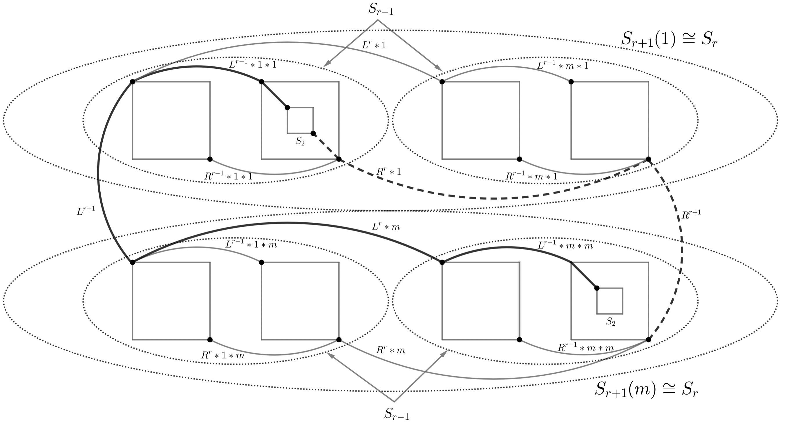
In Figure 4 we illustrate the inductive construction of \(S_{r+1}\), omitting the set of paths \(D(r+1)\) in order to simplify the illustration. The two copies of \(S_{r}\) (namely \(S_{r+1}(1)\) and \(S_{r+1}(m)\)) are encircled by large by dotted ovals, and joined by the paths \(L^{r+1}\) and \(R^{r+1}\). The eight boxes each represent a copy of \(S_{r-2}\). The four horizontally close pairs of these boxes, together with paths \(L^{r-1}\ast B\) and \(R^{r-1}\ast B\), each form a copy of \(S_{r-1}\), where \(B\) is a string of length \(2\) over the letters \(\{1, m\}\) that depends on the pair. The top two copies of \(S_{r-1}\) (i.e. within \(S_{r+1}(1)\)), together with the paths \(L^{r}\ast 1\) and \(R^{r}\ast 1\), form the copy of \(S_{r} \cong S_{r+1}(1)\), while the bottom two copies of \(S_{r-1}\) together with the paths \(L^{r}\ast m\) and \(R^{r}\ast m\) for the copy of \(S_{r} \cong S_{r+1}(m)\).
The \(\ast\) and \(D(r)^{R}\) notation used above are iterated in the natural way. For example, if \(B\) and \(C\) are strings over the letters \(1\) and \(m\), then \((D(r)\ast B)\ast C = D(r)\ast BC\). Also we have \((D(r)\ast B)^{R} = D(r)^{R}\ast B\), \((D(r)^{R})^{R} = D(r)\), and \((D_{1}\cup D_{2})^{R} = D_{1}^{R}\cup D_{2}^{R}\) where \(D_{i}\), \(i = 1,2\) are each \(D(r)\) or \(D(r)^{R}\).
We can decompose \(S_{r+1}\) as follows. Let \(\underline{E_{r+1}} = \cup_{v\in S_{r+1}(1)-X(r+1)} D(v,r+1)\), we have \(S_{r+1} = S_{r+1}(1)\cup S_{r+1}(m)\cup E_{r+1} \cup L^{r+1}\cup R^{r+1} = \big{(}(SQ_{r}\cup D(r))\ast 1\big{)}\cup \big{(}(SQ_{r}\cup D(r)^{R})\ast m\big{)}\cup E_{r+1}\cup L^{r+1}\cup R^{r+1}\).
For the first component on the right we have \((SQ_{r}\cup D(r))\ast 1 = S_{r}\ast 1\), giving us a copy of \(S_{r}\). We now show that the second component is also isomorphic to a copy of \(S_{r}\), which reduces to showing \(SQ_{r}\cup D(r)^{R}\cong S_{r}\). First note that by step \(7\) of the construction we have \(D_{r}^{R} = (D(r-1)^{R}\ast 1)\cup (D(r-1)\ast m)\cup E_{r}^{R}\). Therefore we have \[SQ_{r}\cup D(r)^{R} = \big{(}(SQ_{r-1}\cup D(r-1)^{R})\ast 1\big{)}\cup \big{(}(SQ_{r-1}\cup D(r-1))\ast m\big{)}\cup L^{r}\cup R^{r}\cup E_{r}^{R}.\] Similarly \[SQ_{r}\cup D(r) = \big{(}(SQ_{r-1}\cup D(r-1))\ast 1\big{)}\cup \big{(}(SQ_{r-1}\cup D(r-1)^{R})\ast m\big{)}\cup L^{r}\cup R^{r}\cup E_{r}.\]
We can now construct an isomorphism \(f: SQ_{r}\cup D(r)^{R}\rightarrow SQ_{r}\cup D(r)\) which is a reflection in the \(r\)’th coordinate. Take \(x\in SQ_{r}\cup D(r)^{R}\), so \(x = (x_{1}, x_{2}, \cdots, x_{r-1}, j)\) with \(1\le j\le m\). Then define \(f(x) = (x_{1}, x_{2}, \cdots, x_{r-1}, m – j +1)\). Observe that since \(f\) leaves the first \(r-1\) coordinates undisturbed, we have \(f((SQ_{r-1}\cup D(r-1)^{R})\ast 1) = (SQ_{r-1}\cup D(r-1)^{R})\ast m\) and \(f((SQ_{r-1}\cup D(r-1))\ast m) = (SQ_{r-1}\cup D(r-1))\ast 1\). By this reflection action in the \(r\)’th coordinate, we see that \(f\) reflects the paths \(L^{r}\) and \(R^{r}\) about their midpoints, so that \(f(L^{r}) = L^{r}\) and \(f(R^{r}) = R^{r}\). By the same reflection we see that for any path \(D(v,r)^{R}\in E_{r}^{R}\), \(f(D(v,r)^{R}) = D(v,r)\in E_{r}\), and that \(f\) is then a bijection between \(E_{r}^{R}\) and \(E_{r}\) sending each path \(D(v,r)^{R}\) to its reflection \(D(v,r)\). It follows that \(f(SQ_{r}\cup D(r)^{R}) = SQ_{r}\cup D(r)\) using the decompositions of \(SQ_{r}\cup D(r)^{R}\) and \(SQ_{r}\cup D(r)\) in the preceding paragraph.
The fact that \(f\) is a graph isomorphism is straightforward from its reflection property. We argue just a few typical cases here. For any \(x\in SQ_{r}\cup D(r)^{R}\), write \(x = v_{x}\ast j\), \(1\le j\le m\) with \(v_{x} = (x_{1}, x_{2}, \cdots, x_{r-1})\). First take an edge \(xy\in E(L^{r}\cup R^{r}\cup E_{r}^{R})\). Then \(x = v_{x}\ast j\) and \(y = v_{x}\ast (j+1)\), the case \(y = v_{x}\ast (j-1)\) being similar, and noting that \(v_{x} = v_{y}\). Then \(f(x) = v_{x}\ast (m-j+1)\) and \(f(y) = v_{x}\ast (m-j)\). This shows that if \(xy\in E(L^{r})\) then \(f(x)f(y)\in E(L^{r})\), and the same statement with \(R^{r}\) in place of \(L^{r}\). It also shows that if \(xy\in E_{r}^{R}\), say with \(xy\in E(D(v,r)^{R})\subset E(E_{r}^{R})\), then \(f(x)f(y)\in E(D(v,r))\subset E(E_{r})\). Thus in the case \(xy\in E(L^{r}\cup R^{r}\cup E_{r}^{R})\subset E(SQ_{r}\cup D(r)^{R})\) we have \(f(x)f(y)\in E(L^{r}\cup R^{r}\cup E_{r})\subset E(SQ_{r}\cup D(r))\). As another case suppose \(xy\in E(SQ_{r-1}\cup D(r-1)^{R})\ast 1)\), so \(x = v_{x}\ast 1\) and \(y = v_{y}\ast 1\) and \(v_{x}v_{y}\in E(SQ_{r-1}\cup D(r-1)^{R})\). Then \(f(x)f(y) = (v_{x}\ast m)(v_{y}\ast m)\in E(SQ_{r-1}\cup D(r-1)^{R})\ast m)\). A similar argument shows that \(f\) preserves edges in \(SQ_{r-1}\cup D(r-1))\ast m\).
We now outline briefly how \(f\) preserves nonedges of \(SQ_{r}\cup D(r)^{R}\) in \(P_{m}^{r}\). For brevity let \[B(r) = \big{(} (SQ_{r-1}\cup D(r-1)^{R})\ast 1\big{)}\cup \big{(}(SQ_{r-1}\cup D(r-1))\ast m \big{)}.\]
Nearly the identical proof given for edges shows that \(f\) preserves nonedges of \(SQ_{r}\cup D(r)^{R}\) in \(P_{m}^{r}\) lying in \(B(r)\), based again on the reflection of \(f\). We consider in detail one different case; that is, where a nonedge \(xy\) of \(SQ_{r}\cup D(r)^{R}\) satisfies \(x\in B(r)\) and \(y\notin B(r)\). In this case, \(xy\) is the \(r\)-dimensional nonedge immediately following or preceding a path \(D(w,r)^{R}\). We can take by symmetry \(x = v_{x}\ast m\in (SQ_{r-1}\cup D(r-1))\ast m\) and \(y = v_{y}\ast (m-1)\), with \(v_{x} = v_{y} = (x_{1}, x_{2}, \cdots, x_{r-1})\). Then \(f(x)f(y) = (v_{x}\ast 1)(v_{x}\ast 2)\) which is a nonedge in \(SQ_{r}\cup D(r)\). The remaining cases of nonedges \(xy\) satisfy \(xy\in L^{r}\cup R^{r}\cup E_{r}^{R}\), whose details we omit. The proof that \(f(x)f(y)\) is a nonedge \(SQ_{r}\cup D(r)\) relies on the nonexistence of any edge in \(S_{r}\) with one end in each of two distinct paths \(D(w,r)\) and \(D(w',r)\), or one end in \(L^{r}\cup R^{r}\) and the other in some path \(D(w,r)\).
So our decomposition shows that \(S_{r+1}\) decomposes into two copies of \(S_{r}\) (the subgraphs \(S_{r+1}(1)\) and \(S_{r+1}(m)\)), joined by paths \(L^{r+1}\) and \(R^{r+1}\), together with the subgraph \(E_{r+1}\). Further, \(E_{r+1}\) is a vertex disjoint collection of paths of the form \(D(v, r+1)\), where each such path is pendant on exactly one of \(S_{r+1}(1)\) or \(S_{r+1}(m)\). This is illustrated in Figure 7.
As examples of the \(\lambda\) and \(\rho\) sets, we gave \(\lambda(3)\) and \(\rho(3)\) in step \(6\) of the construction of \(S_{3}\) in the preceding subsection. We also have \[\lambda(4) = \{ (1,1,1,1), (1,1,m,1), (1,1,1,m), (1,1,m,m) \},\] and \[\rho(4) = \{ (m,m,1,1), (m,m,m,1), (m,m,1,m), (m,m,m,m)\}.\]
Our goal now is to show that \(S_{r}\) is an \(S(K_{4})\)-saturated subgraph of \(P_{m}^{r}\). As our first step, we will show that \(S_{r}\) contains no \(S(K_{4})\). For this, we first reduce to showing that the subgraph \(SQ_{r}\) of \(S_{r}\) contains no \(S(K_{4})\). We let \(\underline{[D(r)]}\) be the subgraph of \(S_{r}\) induced by \(V(D(r))\). We call the vertices of \([D(r)]\) connection points of \(S_{r}\), and we call any path in \([D(r)]\) a connection path of \(S_{r}\). We examine \([D(r)]\) for \(r\geq 3\) in the Lemma which follows.
Proof. Recall that we set \([1]_{r} = S_{r}(1)\) and \([m]_{r} = S_{r}(m)\), and \(E_{r} = \cup_{v\in S_{r+1}(1)-X(r)} D(v,r)\).
We proceed by induction on \(r\), starting with the base case \(r = 3\). We have already observed in the proof of Theorem 3.1 that \([D(3)]\) is a forest, each tree component of which is pendant on either \(C_{1}\) or \(C_{2}\), these being the unique cycles of \(S_{3}(1)\) and \(S_{3}(m)\) respectively. So the Lemma holds for \(r = 3\).
Suppose the Lemma holds for \(r\), and consider \([D(r+1)]\). Let \([D(r+1)](1)\) (resp. \([D(r+1)](m)\)) be the copy of \([D(r)]\) in the subgraph \(S_{r+1}(1)\) (resp. \(S_{r+1}(m)\)) of \(S_{r+1}\). Also let \(SQ_{r+1}(1) = SQ_{r}\ast 1\) (resp. \(SQ_{r+1}(m) = SQ_{r}\ast m\)) be the copy of \(SQ_{r}\) in \([1]_{r+1}\) (resp. \([m]_{r+1}\)), so that \(SQ_{r+1} = SQ_{r+1}(1)\cup SQ_{r+1}(m)\cup L^{r+1}\cup R^{r+1}\).
We will use the decomposition \[S_{r+1} = \big{(}(SQ_{r}\cup D(r))\ast 1\big{)}\cup \big{(}(SQ_{r}\cup D(r)^{R})\ast m\big{)}\cup E_{r+1}\cup L^{r+1}\cup R^{r+1},\] given after the construction of \(S_{r}\), where we showed that the \[(SQ_{r}\cup D(r))\ast 1\cong S_{r}\cong (SQ_{r}\cup D(r)^{R})\ast m, \text{ so that }S_{r+1}(1)\cong S_{r}\cong S_{r+1}(m).\]
Applying induction to each of \(S_{r+1}(1)\) and \(S_{r+1}(m)\), we see that \([D(r+1)(1)]\) and \([D(r+1)(m)]\) are forests pendant on \(SQ_{r+1}(1)\) and \(SQ_{r+1}(m)\) respectively. These two forests are vertex disjoint since the last coordinate of any point in the first is \(1\), while the last coordinate of any point in the second is \(m\).
Consider then \(E_{r+1}\), the third union component in \([D(r+1)]\) from step \(7\) of the construction of \(S_{r}\). By construction \(E_{r+1}\) is a vertex disjoint union of paths \(D(v,r+1)\). It suffices to show for each path \(D(v,r+1)\in E_{r+1}\) that either
\(D(v,r+1)\) is itself a tree component of \(D(r+1)\) pendant on \(SQ_{r+1}\), or
\(D(v,r+1)\) is pendant in \(S_{r+1}\) on some tree component \(T'\in D(r+1)(1)\cup D(r+1)(m)\).
In case (2), \(T'\cup D(v,r+1)\) is then a tree component of \(D(r+1)\) inheriting the inductive property from \(T'\) of being pendant on \(SQ_{r+}(1)\cup SQ_{r+}(m)\subset SQ_{r+1}\).
Now path \(D(v,r+1)\) is pendant in \(S_{r+1}\) at either \(v\in S_{r+1}(1)\) or \(v\in S_{r+1}(m)\) (with \(v'\) the point corresponding to \(v\) in \(S_{r+1}(m)\) as in step 6 of the construction of \(S_{r+1}\)), and by symmetry we can take take \(v\in S_{r+1}(1)\). Suppose first that \(v\in D(r+1)(1)\), and by induction let \(T'\) be the tree component of \(D(r+1)(1)\) containing \(v\). Then \(D(v,r+1)\) is pendant on \(T'\), and thus case (2) is satisfied. If \(v\notin D(r+1)(1)\), then by construction \(v\in SQ_{r+1}(1)\). If also \(v\in T'\) for some tree component of \(D(r+1)(1)\), then by induction \(T'\) is pendant in \(S_{r+1}(1)\) (and hence in \(S_{r+1}\)) at \(v\). Since also \(D(v,r+1)\) is also pendant at \(v\), case (2) is satisfied again. Still with \(v\in SQ_{r+1}(1)\), if \(v\) is in no nontrivial tree component of \(D(r+1)(1)\), then clearly \(D(v,r+1)\) is pendant on \(SQ_{r+1}(1)\subset SQ_{r+1}\) at \(v\), and is therefore its own tree component of \(D(r+1)(1)\subset D(r+1)\). So case (1) is satisfied. ◻
For the structure of \(D(r)\), observe first that \(D(2)\) is a disjoint union of paths of the form \(D(v,2)\). We have previously observed in the proof of Theorem 3.1 that \(D(3)\) is a forest each tree component of which is a path or a comb; the latter being a tree \(T\) containing a path \(P\) such that \(T-E(P)\) is a disjoint union of paths, and of course a path being a special case of a comb. The path \(P\) in these nonpath combs \(T\) is a path \(D(v,2)\) for some \(v\). This can be seen in Figure 2, where the path \((2,1,1) \cdots (2,1,m-1)\) plays the role of \(P\) and union of paths \(D(v,3)\), \(v\in P\) and \(v = head(D(v,3))\), together with \(P\) form a tree component which is a comb. For \(D(4)\), the tree components \(T\) are either trees containing a path \(P\) for for which each component of \(T-E(P)\) is a comb, or just paths paths \(D(v,4)\) (for example \(D((m-1, 1, 1, 1),4))\). For general \(D(k)\), each tree component is a nested sequence (in the sense above) of combs up to depth \(k-2\), though we do not use this fact.
In light of Lemma 4.1, for any \(v\in [D(r)]\), let \(T(v)\) be the tree component of \([D(r)]\) containing \(v\). Then let \(\underline{Source(v)}\) be the point of \(SQ_{r}\) at which \(T(v)\) is pendant. As an example, we refer back to Figure 2 and the tree \(H = P\cup \big{(}\cup_{v\in P}D(v,3)\big{)}\), where \(P = (2,1,1) \cdots (2,1,m-1)\) is the path given in the above paragraph. This \(H\) is a tree component of the forest \(D(3)\), and is pendant in \(S_{3}\) at the point \((2,1,1)\). So for every vertex \(x\in H\) we have \(Source(x) = (2,1,1)\). In particular we also have \(Source((2,2,j) = (2,1,1)\) for \(1\le j\le m-1\) and generally for each \(1\le k\le m-1\) we have \(Source((2,k,j) = (2,1,1)\), \(1\le j\le m-1\).
If \(S_{r}\) contains an \(S(K_{4})\), then this \(S(K_{4})\) is a subgraph of \(SQ_{r}\).
For \(z\in [D(r)]\), there is a unique path in \([D(r)]\) from \(Source(v)\) to \(v\).
Proof. For a), any vertex of an \(S(K_{4})\) is contained in a cycle of that \(S(K_{4})\). So by Lemma 4.1 no vertex of \(V(D(r)) – V(SQ_{r})\) of can be in this cycle. Since \(S_{r} = SQ_{r}\cup D(r)\), this \(S(K_{4})\) is a subgraph of \(SQ_{r}\).
Part b) follows immediately from Lemma 4.1 and the fact that \(T(v)\) is a tree. ◻
The arguments in the rest of this section will be inductive, and to facilitate these we introduce here some abbreviated notation for referring to substructures of \(S_{r+1}\).
Since \(r+1\) will be fixed, we will abbreviate \([1]_{r+1}\) and \([m]_{r+1}\) to \([1]\) and \([m]\) respectively. So \([1]\) (resp. \([m]\)) denotes the subgraph \(S_{r+1}(1)\) (resp. \(S_{r+1}(m)\)) of \(S_{r+1}\), this being the subgraph of \(S_{r+1}\) induced by points \(v\) for which \(v_{r+1} = 1\) (resp. \(v_{r+1} = m\)). We let \(\underline{[11]}\) and \(\underline{[1m]}\) be the subgraphs of \(S_{r+1}(1) = [1]\) induced by points \(v\) satisfying \(v_{r} = 1\) and \(v_{r} = m\) respectively, and similarly let \(\underline{[m1]}\) and \(\underline{[mm]}\) be the subgraphs of \(S_{r+1}(m) = [m]\) induced by points \(v\) satisfying \(v_{r} = 1\) and \(v_{r} = m\) respectively. So altogether we have \([1]\cong [m]\cong S_{r}\), while \([ij]\cong S_{r-1}\) for \(i,j \in \{1,m\}\).
The left and right attachment point and path structure is naturally inherited by \([m]\) and \([1]\) as copies of \(S_{r}\) in \(S_{r+1}\), and their subgraphs \([11], [1m]\) etc. as copies of \(S_{r-1}\) in \(S_{r+1}\). The coordinates in \(S_{r+1}\) of such points are obtained by taking the coordinates of the attachment point in \(S_{r}\) (or \(S_{r-1}\)) and appending the appropriate coordinate suffix in \(S_{r+1}\). So we have \[\begin{aligned}L([1]) =& 1^{r}1 = 1^{r+1} = L(S_{r+1}),\\ R([1]) =& m^{r}1,\\ L([m]) =& 1^{r}m,\\ R([m]) =& m^{r}m = m^{r+1} = R(S_{r+1}),\end{aligned}\] and for \(i, j = 1\) or \(m\) we have \[\begin{aligned} L([ij]) =& 1^{r-1}ji,\end{aligned}\] and \(R([ij]) = m^{r-1}ji.\) So we have \[\begin{aligned} L([11]) = &L([1]),\\ R([11]) =& m^{r-1}11 = m^{r-1}1^{2},\\ L([1m]) =& 1^{r-1}m1,\\ R([1m]) =& m^{r-1}m1 = m^{r}1,\\ L([m1]) =& 1^{r-1}1m = 1^{r}m,\\ R([m1]) =& m^{r-1}1m,\\ L([mm]) =& 1^{r-1}mm = 1^{r-1}m^{2},\end{aligned}\] and \[\begin{aligned}R([mm]) =& m^{r-1}mm = m^{r+1} = R(S_{r+1}). \end{aligned}\]
Similarly the attachment paths \(L^{r}\) and \(R^{r}\) in \(S_{r}\) appearing in the copy \(S_{r+1}(1)\cong S_{r}\) (resp. \(S_{r+1}(m)\cong S_{r}\) of \(S_{r}\) will be written as \(L^{r}\ast 1\) and \(R^{r}\ast 1\) (resp. \(L^{r}\ast m\) and \(R^{r}\ast m\)) as in step \(4\) of the construction of \(S_{r}\).
The various left and right attachment paths, all of length \(m-1\), join pairs of these attachment points. For example, \(L^{r+1}\) joins \(L([11])\) to \(L([m1])\), and \(R^{r+1}\) joins \(R([1m])\) to \(R([mm])\). Now let \(L^{r}([i]) = L^{r}\ast i\) and \(R^{r}([i])\ast i\) be the left and right attachment paths in \([i]\), \(i = 1,m\). Then \(L^{r}([i])\) joins \(L([i1])\) to \(L([im])\), and \(R^{r}([i])\) joins \(R([i1])\) to \(R([im])\).
Toward showing that \(S_{r}\) is \(S(K_{4})\)-saturated in \(P_{m}^{r}\) we begin by proving that \(S_{r}\) contains no \(S(K_{4})\). Recall that the points of degree \(3\) in an \(S(K_{4})\) are called junction points or just junctions, and we call the six internally disjoint paths in this \(S(K_{4})\) joining the pairs of junctions junction paths.
Proof. By Corollary 4.2, it suffices to show that \(SQ_{r}\) contains no \(S(K_{4})\). We proceed by induction on \(r\), having proved the base case \(r = 3\) in Theorem 3.1. Assume the Theorem is true for \(SQ_{t}\), \(t\le r\), and we prove it for \(SQ_{r+1}\). We begin with the following claim.
Proof. We proceed by induction. The claim is vacuously true for \(r=3\) since \(SQ_{3}\) contains no \(S(K_{4})\). Now assume the claim true for \(SQ_{r}\), \(r\geq 3\), and consider now the clam for \(SQ_{r+1}\). We write \(SQ_{r+1}(i)\) (resp. \(SQ_{r+1}(ij)\)) for the subgraph \(SQ_{r+1}\cap [i]\) (resp. \(SQ_{r+1}\cap [ij]\)), \(i,j = 1\) or \(m\).
Suppose to the contrary that all four junctions of \(S\) lie in \(SQ_{r+1}(1)\) (symmetrically in \(SQ_{r+1}(m)\)).
Proof. By the first inductive assumption that \(SQ_{r}\) contains no \(S(K_{4})\), we have \(S\not\subset SQ_{r+1}(1)\cong SQ_{r}\). So \(S\cap SQ_{r+1}(m) \ne \emptyset\). Hence there is a junction path \(P\subset S\) which leaves \(SQ_{r+1}(1)\), enters \(SQ_{r+1}(m)\), and then returns to \(SQ_{r+1}(1)\). So \(P\) contains the subpaths \(L^{r+1}\) and \(R^{r+1}\), and hence there can be only one such junction path. If not, then some other junction path leaving and reentering \(SQ_{r+1}(1)\) must also use \(L^{r+1}\) and \(R^{r+1}\) and yet be internally disjoint from \(P\), a contradiction. ◻
Proof. Assume to the contrary that all four junctions lie in \(SQ_{r+1}(11)\), with a symmetric argument if they all lie in \(SQ_{r+1}(1m)\). With \(P\) as in the statement of Subclaim 4.5, we regard \(P\) as leaving \(SQ_{r+1}(11)\) on \(L^{r+1}\) to arrive at \(L([m1])\), passing through \(SQ_{r+1}(m)\) on some path \(X\) from \(L([m1])\) to \(R([mm])\), and finally returning to \(SQ_{r}(1)\) along \(R^{r+1}\). Now \(X\) can take essentially one of the two following forms: ◻
a path \(Y\subset SQ_{r+1}(m1)\) from \(L([m1])\) to \(R([m1])\), followed by the path \(R^{r}([m])\) from \(R([m1])\) to \(R([mm])\) (illustrated in Figure 5), or
the path \(L^{r}([m])\) from \(L([m1])\) to \(L([mm])\) followed by a path \(Y'\subset SQ_{r+1}(mm)\) from \(L([mm])\) to \(R([mm])\).
The choices of \(A\) or \(B\) lead to symmetric arguments later, and we will address only choice A here. We note that the existence of \(Y\) in choice (A) and of \(Y'\) in choice B is ensured by Lemma 4.9b, which follows and is independent of this Theorem. Now \(P\) must finally return to \(SQ_{r+1}(11)\) via either the path \(L^{r}([1])\) or the path \(R^{r}([1])\). If \(L^{r}([1])\subset P\) then \(P\) would intersect itself at the endpoint \(L([1])\) of \(L^{r}([1])\cap L^{r+1}\), a contradiction. So we have \(R^{r}([1])\subset P\). Then \(P\cap SQ_{r+1}(1m) = R([1m])\). This is because \(P\) cannot cross itself and also cannot exit \([1m]\) through \(L([1m])\) since as just shown \(L^{r}([1])\not\subset P\). So after passing through \(R^{r}([1])\), \(P\) reenters \(SQ_{r+1}(11)\) at \(R([11])\) and continues with a subpath \(Q\subset SQ_{r+1}(11)\) going from \(R([11])\) to one of the two junction points, call it \(p_{1}\), of \(S\) joined by \(P\). Letting \(p_{2}\) be the other of these two junctions, we can write \(P\), with choice A above, as \(P = F-L^{r+1}-Y-R^{r}([m])-R^{r+1}-R^{r}([1])-Q\), where \(F\) is the subpath of \(P\) joining \(p_{2}\) to \(L([11]))\). This \(P\) is illustrated in Figure 5.

Proof. Suppose to the contrary that some junction path \(A\) leaves \(SQ_{r+1}(11)\). Then \(A\) must leave and then reenter \(SQ_{r+1}(11)\) by the contrary assumption to Subclaim 4.6 that that all four junctions lie in \(SQ_{r+1}(11)\). So \(A\) must contain two of the of the three entry/exit paths \(\{ L^{r}([1]), L^{r+1}, R^{r}([1]) \}\) into \(SQ_{r+1}(11)\). But \(P\) already contains two of these paths, contradicting that \(A\) and \(P\) are internally disjoint. ◻
We can now complete the proof of Subclaim 4.6. We still refer to the junction path \(P\) of Subclaim 4.5. We “splice out” the subpath \(P' = L^{r+1}-Y-R^{r}([m])-R^{r+1}\) from \(P\), and replace it by the dashed subpath \(T-L^{r}([1])\) contained in \(SQ_{r+1}(1)\), as illustrated in Figure 5 and described as follows. Take any path \(T\) in \(SQ_{r+1}(1m)\) with ends \(L([1m])\) and \(R([1m])\), noting that such a \(T\) exists by Lemma 4.9 which is proved after and independently of this Theorem. Now replace \(P'\) in \(P\) by the path \(L^{r}([1]) – T\), observing that \(P'\) and \(L^{r}([1]) – T\) have the same two endpoints \(L([11])\) and \(R([1m])\). So we obtain the new path \(P+ = F – L^{r}([1]) – T – R^{r}([1]) – Q\), so \(P+ \subset SQ_{r+1}(1)\).
We claim that \(P+\) can be taken as a junction path replacing \(P\) in \(S\). First, \(P+\) joins the same two vertices \(p_{1}\) and \(p_{2}\) that \(P\) does. Note also that the subpath \(L^{r}([1]) – T\) of \(P+\) has no internal intersection with other junction paths of \(S\) since such intersections, apart from possibly \(L([11])\), are disallowed by the Observation above, and for \(L([11])\) disallowed by the original internal disjointness of \(P\) with other junction paths. The other three subpaths of \(P+\), namely \(F\), \(R^{r}([1])\), and \(Q\), also have no such internal intersections since these were already subpaths of \(P\) which had no such intersections. Therefore \(P+\) is indeed a path which is internally disjoint from the other junction paths of \(S\), and hence can act as a junction path in \(S\) replacing \(P\). Since \(P\) was the only junction path leaving \(SQ_{r+1}(1)\) by Subclaim 4.5, this replacement results in a copy \(S'\) of \(S(K_{4})\) lying entirely in \(SQ_{r+1}(1)\cong SQ_{r}\), contradicting the inductive hypothesis of the Theorem that \(SQ_{r}\) contains no copy of \(SK_{4}\). So Subclaim 4.6 is proved. (end of proof of Subclaim 4.6).
We can now complete the proof of the Claim, still working with the contrary assumption that all four junctions of \(S\) lie in \(SQ_{r+1}(1)\). By Subclaim 4.6 we need only consider the two nontrivial partitions of the junctions among \(SQ_{r+1}(11)\) and \(SQ_{r+1}(1m)\).
Suppose first that each of \(SQ_{r+1}(11)\) and \(SQ_{r+1}(1m)\) contain two junctions. Then there must be at least four internally disjoint junction paths exiting \(SQ_{r+1}(1m)\) and ultimately entering \(SQ_{r+1}(11)\). Now any path exiting \(SQ_{r+1}(1m)\) and eventually entering \(SQ_{r+1}(11)\) must have as a subpath exactly one of the three exit paths from \(SQ_{r+1}(1m)\) in \(SQ_{r+1}\); these being \(R^{r+1}, R^{r}([1])\), and \(L^{r}([1])\). By the Pigeon Hole principle two of these junction paths share one of these exit paths, contradicting their internal disjointness.
So we can assume by symmetry that \(SQ_{r+1}(1m)\) contains a single junction \(x\) while \(SQ_{r+1}(11)\) contains the other three junctions of \(S\). Then there must be three internally disjoint junction paths having only vertex \(x\) in common leaving \(SQ_{r+1}(1m)\) and eventually entering \(SQ_{r+1}(11)\). Hence the three paths \(R^{r+1}, R^{r}([1])\), and \(L^{r}([1])\) are distributed in a one to one way as subpaths of the three internally disjoint junction paths from \(x\). One of these junction paths, call it \(P_{1}\), contains \(R^{r+1}\), passes through \(SQ_{r}(m)\), and must enter \(SQ_{r+1}(11)\) along the subpath \(L^{r+1}\). A second such junction path, call it \(P_{2}\), enters \(SQ_{r+1}(11)\) along the subpath \(L^{r}([1])\). But then \(L([11])\in P_{1}\cap P_{2}\), a contradiction since these three paths can have only vertex \(x\) in common. ◻
Returning to the proof of the theorem, assume to the contrary that \(SQ_{r+1}\) contains a copy \(S\) of an \(S(K_{4})\). By the preceding claim each of \(SQ_{r+1}(1)\) and \(SQ_{r+1}(m)\) contains at least one junction of \(S\). So there must be at least three junction paths of \(S\) joining junctions in \(SQ_{r}(m)\) to junctions in \(SQ_{r}(1)\). But each of these three paths contains exactly one of the two paths \(L^{r+1}\) or \(R^{r+1}\), the latter being the only exit paths from \(SQ_{r}(m)\) in \(SQ_{r+1}\). By the Pigeon Hole principle this contradicts the internal disjointness of the three junction paths, completing the proof of the theorem. ◻
To complete the proof that \(S_{r}\) is \(S(K_{4})\)-saturated in \(P_{m}^{r}\), it remains to prove the nonedge addition property. To that end, we will need a Lemma on the path structure in \(S_{r}\).
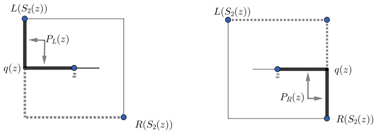
There exists a path \(P\subset S_{r}\) from \(L(S_{r})\) to \(L(S_{2})\) (resp. \(R(S_{r})\) to \(R(S_{2})\)) which is a concatenation of left attachment paths (resp. right attachment paths).
There is a path from \(R(S_{r})\) to \(L(S_{r})\) which is a concatenation of right attachment paths (paths in \(\pi_{R}(r)\)) from \(R(S_{r})\) to \(R(S_{2})\), followed by a path in \(S_{2}\) along \(C\) from \(R(S_{2})\) to \(L(S_{2})\), followed by a concatenation of left attachment paths (paths in \(\pi_{L}(r)\)) from \(L(S_{2})\) to \(L(S_{r})\).
Let \(z\in V(S_{2})\), \(z\notin \{ L(S_{2}), R(S_{2}) \}\). Then \(P_{L}(z)\) (resp. \(P_{R}(z)\)) passes through \(q(z)\) and avoids \(R(S_{2})\) (resp. \(L(S_{2})\)).
With \(z\) as in c), there is a path in \(S_{2}\) along \(C\) from \(R(S_{2})\) (resp. \(L(S_{2})\)) to \(q(z)\) intersecting \(P_{L}(z)\) (resp. \(P_{R}(z)\)) only at \(q(z)\).
Proof. In this proof we will refer to subgraphs \(S_{2}\ast B_{r-2}\) or \(L^{j}\ast B_{r-j}\) in \(S_{r}\), for suffixes \(B_{r-2}\) or \(B_{r-j}\) of length \(r-2\) or \(r-j\) (resp.) over the letters \(1\) and \(m\), by their isomorphic copies \(S_{2}\) or \(L^{j}\) for brevity. These suffixes locate the copy of \(S_{2}\) or \(L^{j}\) within \(S_{r}\), but that location is not important for this proof.
Starting with part a) we prove the statement for the path from \(L(S_{r})\) to \(L(S_{2})\), where the proof for the path from \(R(S_{r})\) to \(R(S_{2})\) is identical with the obvious changes. We proceed by induction on \(r\). In the base case \(r = 3\), \(S_{3}\) contains just the two squares \(S_{3}(1)\) and \(S_{3}(m)\), each isomorphic to \(S_{2}\). Noting that \(L(S_{3}) = L(S_{3}(1))\), the required path is then given by \(L^{3}\) joining \(L(S_{3})\) and \(L(S_{3}(m))\) in the construction of \(S_{3}\).
For the inductive step, assume the theorem true for \(S_{r}\) and consider \(S_{r+1}\) with its two subgraphs \(S_{r+1}(1)\) and \(S_{r+1}(m)\), each isomorphic to \(S_{r}\). We have \(S_{2}\subset S_{r+1}(1)\) or \(S_{2}\subset S_{r+1}(m)\). If \(S_{2}\subset S_{r+1}(1)\cong S_{r}\), again noting that \(L(S_{r+1}) = L(S_{r+1}(1))\) we obtain the required concatenation of left attachment paths \(P = L^{r_{1}}L^{r_{2}}\cdots L^{3} \subset S_{r+1}(1)\), for some sequence of integers \(r\geq r_{1}> r_{2} \cdots > 3\), by applying the inductive hypothesis.
Now suppose \(S_{2}\subset S_{r+1}(m)\). By induction there is a path \(P'\subset S_{r+1}(m)\) consisting of a concatenation of left attachment paths joining \(L(S_{r+1}(m))\) to \(L(S_{2})\). Recall that by construction of \(S_{r+1}\), the path \(L^{r+1}\) joins \(L(S_{r+1}) = L(S_{r+1})(1)\) to \(L(S_{r+1}(m))\). Then we obtain the concatenation \(P = L^{r+1}P'\) of left attachment paths joining \(L(S_{r+1})\) to \(L(S_{2})\), completing the inductive step.
For part b), again we proceed by induction. In the base case \(r = 3\), for the required \(R(S_{3}) – L(S_{3})\) path we take the path from \(R(S_{3}) = R(S_{3}(m))\) to \(L(S_{3}(m))\) around the cycle of \(S_{3}(m)\), followed by the path \(L^{3}\) joining \(L(S_{3}(m))\) to \(L(S_{3}(1))\). Here the right attachment path in the statement can be taken as the trivial one consisting of just the point \(R(S_{3}(m))\) itself.
For the inductive step we assume the theorem true for \(S_{r}\). If \(S_{2}\subset S_{r+1}(m)\), then apply induction to find the required path \(P\) in \(S_{r+1}(m)\) from \(R(S_{r+1}(m)) = R(S_{r+1})\) to \(L(S_{r+1}(m))\) passing through \(S_{2}\) as required. Now concatenate \(P\) with the left attachment path \(L^{r+1}\) joining \(L(S_{r+1}(m))\) to \(L(S_{r+1}(1))\) given in the construction of \(S_{r+1}\) to obtain the required concatenated path \(L^{r+1}P\) joining \(R(S_{r+1})\) to \(L(S_{r+1})\) for part b). If \(S_{2}\subset S_{r+1}(1)\), then we begin with the path \(R^{r+1}\) joining \(R(S_{r+1}(m))\) and \(R(S_{r+1}(1))\) given in the construction of \(S_{r+1}\). Now apply induction to get a path \(Q\) in \(S_{r+1}(1)\) joining \(R(S_{r+1}(1))\) and \(L(S_{r+1}(1)) = L(S_{r+1})\) and passing through \(S_{2}\). Then the concatenation \(R^{r+1}Q\) gives the required path in \(S_{r+1}\) joining \(R(S_{r+1})\) to \(L(S_{r+1})\) for part b).
An illustration of the concatenations of paths in parts a) and b) of the Lemma is given in Figure 4, these concatenations shown in bold and dashed curves. An accompanying description is given immediately following the proof of this Lemma.
For parts c) and d), we refer the reader to Figure 6 which illustrates the proofs which follow.
Consider part c). If \(z\notin C\), then \(z\) is on a pendant path from \(C\), so both \(P_{L}(z)\) and \(P_{R}(z)\) must contain \(q(z)\). Also \(P_{L}(z)\) consists of this pendant path followed by the shorter of the two paths on \(C\) from \(q(z)\) to \(L(S_{2})\). Therefore \(P_{L}(z)\) avoids \(R(S_{2})\), and \(P_{R}(z)\) avoids \(L(S_{2})\). If \(z\in C\), then \(q(z) = z\) and the claims on \(P_{L}(z)\) and \(P_{R}(z)\) are then obvious for the same reasons.
Consider part d). By part c) and the definition of \(P_{L}(z)\), the shortest path from \(R(S_{2})\) to \(q(z)\) (which runs along \(C\)) is the path required in part d). The proof for \(P_{R}(z)\) is just obtained by the obvious interchange of \(L(S_{2})\) with \(R(S_{2})\), and of \(P_{L}(z)\) with \(P_{R}(z)\). ◻
Figure 4 illustrates concatenations of left and right attachment paths (in bold and dashed curves) claimed to exist in parts a) and b) of this Lemma. For a concatenation of left attachment paths from \(L(S_{r+1})\) to \(L(S_{2})\) ( as in part a) ) observe the sequence of paths starting at the upper left corner which is the vertex \(L(S_{r+1})\). One such concatenation begins with the left attachment path \(L^{r-1}\ast 1\ast 1\) followed by a an inductively constructed concatenation of such paths (indicated by the oblique line) within the upper and second from left copy of \(S_{r-2}\) ending at the vertex \(L(S_{2})\) of the \(S_{2}\) within that copy of \(S_{r-2}\) in the figure. Another example again begins at \(L(S_{r+1})\), and proceeds along the left attachment paths in the order \(L^{r+1} – L^{r}\ast m – L^{r-1}\ast m\ast m\) and finally along a an inductively constructed concatenation of left attachment paths (again shown as an oblique line) within the lower and rightmost copy of \(S_{r-2}\), leading to \(L(S_{2})\). Finally observe the concatenation of right and left attachment paths going from \(R(S_{r+1})\) (the corner point at lower right) to \(L(S_{r+1})\) (the corner point at upper left) as in part b) of the Lemma. This begins with the succession of two right attachment paths \(R^{r+1} – R^{r}\ast 1\) followed by the inductively constructed concatenation of right attachment paths within the upper second from left copy of \(S_{r-2}\), leading to \(R(S_{2})\) (all in dashed curves), followed by the cycle around \(S_{2}\), followed by the reverse of the concatenation of the first two left attachment paths given in the first example, leading to \(L(S_{r+1})\).
In our next theorem we show that the edge addition property holds in \(S_{r}\); that is, that for any nonedge \(e\) of \(S_{r}\) in \(P_{m}^{r}\) we have \(S(K_{4})\subset S_{r}+e\). The proof will be by induction on \(r\), and to facilitate that induction we need the following definitions and notation.
We continue with the notation \(A \xrightarrow{\:\text{S} \:} B\) and its concatenation used previously in the analysis of \(S_{3}\). We extend here the meaning of symbol \(S\) to include not only the name of a path joining vertices \(A\) and \(B\), but also the name of a Lemma or construction justifying the existence of such a path. So \(S\) can take values \(La, Lb, Lc, Ld\) to indicate Lemma 4.9 parts \(a,b,c,d\) respectively, or \(L'a, L'b\) to indicate Corollary 4.2 parts \(a,b\) respectively, or just the name of some path – usually some attachment path such as \(L^{r+1}\), \(L^{r}\ast 1\subset [1]\), or \(L^{r}\ast m\subset [m]\).
Proof. We proceed by induction. The theorem has been proved for \(r = 3\) in Theorem 3.1. Assume the theorem true for \(S_{k}\), \(3\le k\le r\), and we prove it for \(S_{r+1}\). With the notation given just before this theorem, we have the following decompositions:
\[\begin{aligned} [1] =& [11]\cup [1m]\cup \{ D(v,r): \big{(}v\in V([11])\cup V([1m])\big{)} – X(r)\}\cup (L^{r}\ast 1)\cup (R^{r}\ast 1) \cong S_{r},\\ [m] = &[m1]\cup [mm]\cup \{ D(v,r)^{R}: \big{(}v\in V([m1])\cup V([mm])\big{)} – X(r)\} \cup (L^{r}\ast m)\cup (R^{r}\ast m) \cong S_{r},\\ S_{r+1} =& [1]\cup [m]\cup \{ D(v,r+1): \big{(}v\in V([1])\cup V([m])\big{)} – X(r+1)\} \cup L^{r+1}\cup R^{r+1}. \end{aligned}\]
These decompositions are illustrated in Figure 7. On the left you see the decomposition of \(S_{r+1}\) into four copies of \(S_{r-1}\), the top two being \([11]\) and \([1m]\) contained in \([1]\), and the bottom two being \([m1]\) and \([mm]\) contained in \([m]\), together with various attachment paths. The attachment paths \(L^{r+1}\) and \(R^{r+1}\) link \([1]\) with \([m]\), while the attachment paths \(L^{r}\ast 1\) and \(R^{r}\ast 1\) link \([11]\) and \([1m]\), and \(L^{r}\ast m\) and \(R^{r}\ast m\) link \([m1]\) and \([mm]\). Those connection paths in \(D(r+1)\) lying outside the four copies of \(S_{r-1}\) are excluded for simplicity, but are included in the right Figure 8. Figure 8 shows paths of the form \(D(v,r+1)\) running between \([1]\) and \([m]\), and paths of the form \(D(v,r)\ast 1\) running between \([11]\) and \([1m]\) together with paths \(D(v,r)^{R}\ast m\) running between \([m1]\) and \([mm]\).
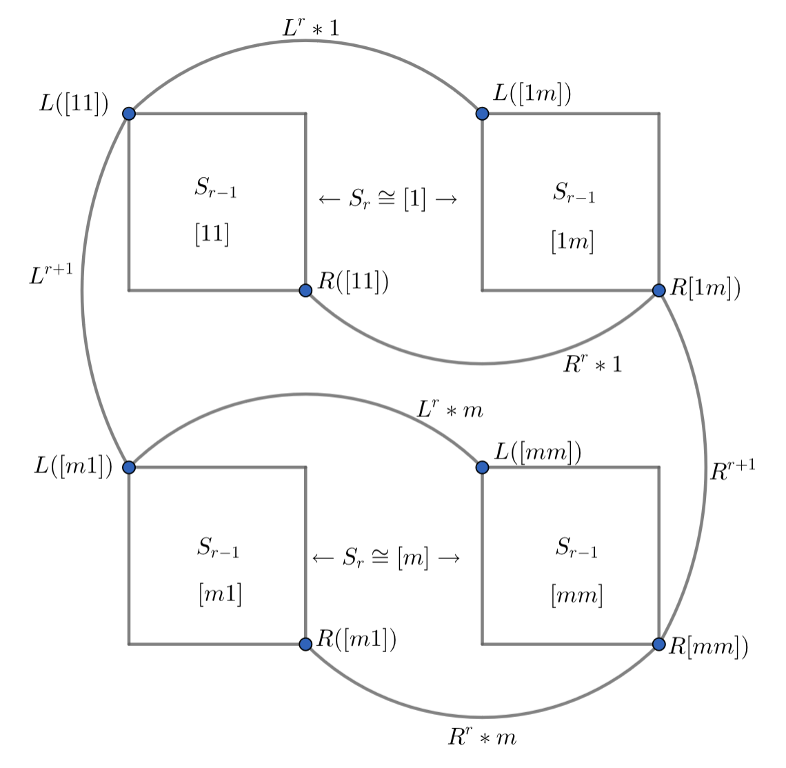
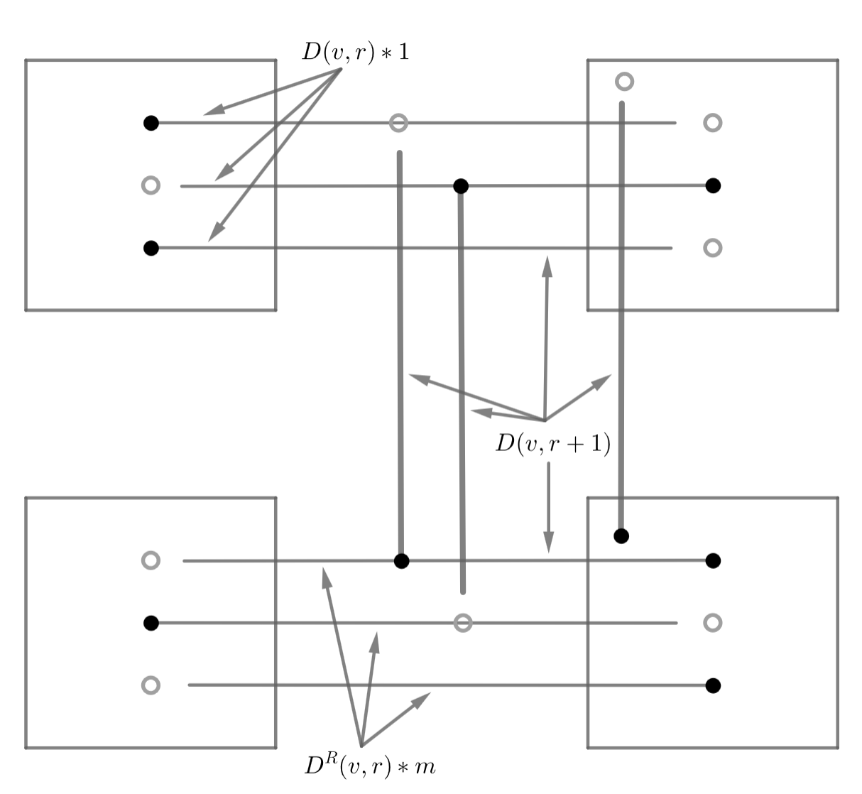
Let \(e = vw\) be any nonedge of \(S_{r+1}\) in \(P_{m}^{r+1}\). If both \(v,w\in [1]\) or both \(v,w\in [m]\), then we are done by the inductive hypothesis as applied to \([1]\) or \([m]\) since \([1]\cong [m]\cong S_{r}\). Further we cannot have \(v\in [1]\) and \(w\in [m]\) since then \(|v_{r+1} – w_{r+1}| = m-1\), while at the unique coordinate where \(v\) and \(w\) disagree the difference must be \(1\), a contradiction. Thus either \(\{v,w\}\cap \big{(}[m]\cup [1]\big{)} = \emptyset\) or exactly one of \(\{v,w\}\) lies in \([m]\cup [1]\).
Let the nonedge \(e = vw\) be \(k\)-dimensional. We argue according to the value of \(k\). In the body of this proof we treat only the case \(k = r + 1\), and provide the similar details for the case \(k\le r\) in Appendix II.
The assumption \(k = r + 1\), together with \(vw\) being a nonedge, implies that \(vw\) is the unique nonedge of dimension \(r+1\) following or preceding a \(D\)-path, call it \(D(v', r+1)\), of dimension \(r+1\). By symmetry we can take \(v'\in [m]\) and \(v' = head(D(v', r+1))\), so that \(w = tail(D(v', r+1))\in [1]\). So in this case exactly one of \(\{v,w\}\) lies in \([m]\cup [1]\), this being \(w\in [1]\). The situation so far is illustrated in Figure 9, where additional aspects of that Figure will be explained soon. We have two possibilities; either \(v'\in [D(r+1)](m)\) or \(v'\in SQ_{r+1}(m)\). For convenience, set \(D'(r+1) = D(r+1) – \big{(}[1]\cup [m] \big{)}\), so that in each case we have \(v\in D'(r+1)\).
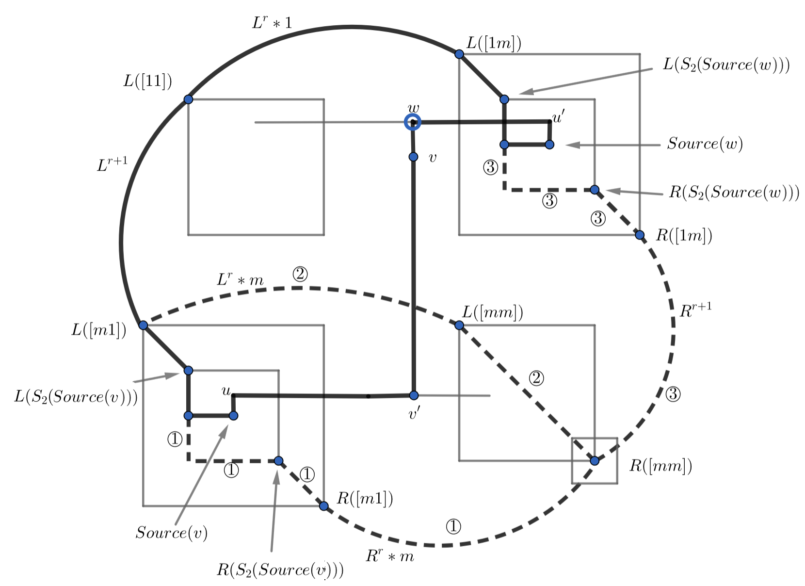
Assume first that \(v'\in [D(r+1)](m)\). Since \(v' = head(D(v',r+1))\in [m]\) we have \(Source(v) = Source (v')\in [m1]\) or \([mm]\), and by symmetry we can suppose that \(Source(v)\in [m1]\).
We now show that \(Source(w)\in [1m]\). Now \(v'\) lies on some \(D\)-path of dimension \(r\), call it \(D(u,r)\ast m\), with \(u = head(D(u,r))\in [m1]\) since \(Source(v)\in [m1]\). This \(D(u,r)\ast m\) is portrayed as the horizontal line through \(v'\) in Figure 9, of which the bolded part is the subpath \(D(u,r)\) joining \(u\) and \(v'\). Similarly there is a \(D\)-path of dimension \(r\), call it \(D(u',r)\ast m\) passing through \(w\), portrayed as the horizontal line through \(w\) in Figure 9. But \(v'\) and \(w\) are corresponding points in \([m]\) and \([1]\) (resp.). So we have \(D(u',r) = D(u,r)^{R}\) by construction. Since \(head(D(u,r))\ast m)\in [m1]\) we get \(head(D(u',r))\ast 1)\in [1m]\), so \(u'\in [1m]\) and it follows that \(Source(w)\in [1m]\).
Recall that \(Source(v)\) and \(Source(w)\) are in \(SQ_{r+1}\) by definition, so each of these points is either in a square \(S_{2}\) or in some attachment path \(L^{t}\) or \(R^{t}\), \(3\le t < r\). For the bound \(t < r\), observe first that \(t\ne r+1\) since by construction there are points \(x\in L^{r+1}\cup R^{r+1}\) for which \(D(x,r+1)\) is defined. Also \(t\ne r\) since \(v\in D(r+1)\).
In the constructions which follow we will suppose that each of \(Source(v)\) and \(Source(w)\) is in its own square, and later we treat briefly the case where each of \(Source(v)\) and \(Source(w)\) is in some attachment path \(L^{t}\) or \(R^{t}\) by a small modification. Given the reduction in the preceding paragraph, we then have \(S_{2}(Source(v))\subset [m1]\) and \(S_{2}(Source(w))\subset [1m]\).
We then obtain an \(S(K_{4})\subset S_{r+1} + vw\), as illustrated in Figure 9 and described formally as follows. Define a cycle \(W\subset S_{r+1}+vw\) containing \(vw\), indicated in bold lines in Figure 9, as follows. \[\begin{aligned}W =& v – w \xrightarrow{\:\text{L'b} \:} Source(w) \xrightarrow{\text{\: Lc \:}} L(S_{2}(Source(w))) \xrightarrow{\:\text{La} \:} L([1m]) \xrightarrow{\:\text{$L^{r}\ast 1$} \:} L([11])\\ &\xrightarrow{\:\text{$L^{r+1}$} \:} L([m1]) \xrightarrow{\:\text{La} \:} L(S_{2}(Source(v))) \xrightarrow{\text{\: Lc \:}} Source(v) \xrightarrow{\: \text{L'b} \:} v.\end{aligned}\]
We describe here in prose the use of the arrow notation above to describe \(W\), to further familiarize the reader with this notation. Here starting with the edge \(vw\), we follow the connection path \(w \xrightarrow{\:\text{L'b} \:} Source(w)\) joining \(w\) and \(Source(w)\) in \([D(r)]\ast 1\) given by Corollary 4.2b, followed by the path \(Source(w) \xrightarrow{\text{\: Lc \:}} L(S_{2}(Source(w)))\) given in Lemma 4.9c. This then is followed by a succession of left attachment paths all guaranteed to exist either by Lemma 4.9a or the construction of \(S_{r}\) and \(S_{r+1}\). These are, in the order they appear on \(W\), given by \(L(S_{2}(Source(w))) \xrightarrow{\:\text{La} \:} L([1m])\), \(L([1m]) \xrightarrow{\:\text{$L^{r}\ast 1$} \:} L([11])\), \(L([11])\xrightarrow{\:\text{$L^{r+1}$} \:} L([m1])\), \(L([m1]) \xrightarrow{\:\text{La} \:} L(S_{2}(Source(v)))\). These are followed by the path \(L(S_{2}(Source(v))) \xrightarrow{\text{\: Lc \:}} Source(v)\) justified by Lemma 4.9c, and then the cycle is completed by the connection path \(Source(v) \xrightarrow{\: \text{L'b} \:} v\) given in Corollary 4.2b, the latter path passing through \(u\) and \(v'\) as shown in the Figure.
We now take the point \(R([mm])\), knowing that \(R([mm])\notin W\) since by construction \(W\) never enters \([mm]\). The three independent \(R([mm])-W\) paths required to complete the construction of an \(S(K_{4})\subset S_{r+1}+vw\), indicated in numbered dashed curves and lines in Figure 9, are as follows.
\[\begin{aligned}P_{1} =& R([mm]) \xrightarrow{\:\text{$R^{r}\ast m$} \:} R([m1]) \xrightarrow{\:\text{La} \:} R(S_{2}(Source(v))) \xrightarrow{\:\text{Ld} \:} q(Source(v)),\\ &\text{(intersecting $W$ at $q(Source(v))$)},\\ P_{2} =& R([mm]) \xrightarrow{\:\text{Lb} \:} L([mm]) \xrightarrow{\:\text{$L^{r}\ast m$} \:} L([m1]), \text{(intersecting $W$ at $L([m1])$)},\\ P_{3} =& R([mm]) \xrightarrow{\:\text{$R^{r+1}$} \:} R([1m]) \xrightarrow{\:\text{La} \:} R(S_{2}(Source(w))) \xrightarrow{\:\text{Ld} \:} q(Source(w)), \\ &\text{(intersecting $W$ at $q(Source(w))$)}.\end{aligned}\]
We give the proof of independence of the paths \(P_{i}\), \(1\le i\le 3\) in Appendix I. For the remainder of this section we omit such independence proofs as they are very similar to the one given there.
We now indicate briefly the adjustment to the constructions above that will cover the case where each of \(Source(v)\) and \(Source(w)\) is on some attachment path. Suppose for example that \(Source(v)\in L^{t}\subset SQ_{r+1}(m1)\). This \(L^{t}\) is a left attachment path joining the two left attachment points \(L(S_{t}(1))\) and \(L(S_{t}(m))\) in some subgraph \(S_{t}\subset [m1]\), \(t < r\). It is useful here to refer again to Figure 9, where we now replace \(S_{2}(Source(v))\) by \(S_{t}(1)\), and we imagine the left attachment path \(L^{t}\) as joining \(L(S_{t}(1))\) to the point \(L(S_{t}(m))\) (where neither \(L^{t}\) nor \(S_{t}(m)\) is visible in the Figure). Since \(Source(v)\) is on this \(L^{t}\), we now reroute \(W\) (with the help of Lemma 4.9a) so that \(W\) arrives at \(L(S_{t}(1))\) and from there reaches \(Source(v)\) along the path \(L^{t}\) incident on \(L(S_{t}(1))\). The arrival at \(L(S_{t}(1))\) is accomplished by viewing \(L(S_{t}(1))\) as the left attachment point of the square containing it, that is by observing that \(L(S_{t}(1)) = L(S_{2}(L(S_{t}(1))))\), and then applying Lemma 4.9a. Explicitly then, we replace the subpath \(L([m1]) \xrightarrow{\:\text{La} \:} L(S_{2}(Source(v))) \xrightarrow{\text{\: Lc \:}} Source(v)\) of the current \(W\) by the path \(L([m1]) \xrightarrow{\:\text{La} \:} L(S_{t}(1)) \xrightarrow{\text{\: $L^{t}$ \:}} Source(v)\), leaving the rest of \(W\) unchanged. Call the new cycle \(W'\).
We now also reroute the path \(P_{1}\) so that it now intersects \(W'\) at \(Source(v)\in [m1]\), calling the rerouted path \(P_{1}'\), as follows. Now \(P_{1}'\) will still begin at \(R([mm])\), with the goal of \(P_{1}'\) intersecting \(W'\) at \(Source(v)\). We do this by moving \(P_{1}'\) through a sequence of right attachment paths, using Lemma 4.9b, to reach \(L(S_{t}(m))\) (similarly regarded as \(L(S_{2}(L(S_{t}(m))))\) in applying Lemma 4.9b). Then \(P_{1}'\) reaches \(Source(v)\) along the path \(L^{t}\) incident to \(L(S_{t}(m))\). Explicitly we replace the subpath \(R([m1]) \xrightarrow{\:\text{La} \:} R(S_{2}(Source(v))) \xrightarrow{\:\text{Ld} \:} q(Source(v))\) of \(P_{1}\) by the path \(R([m1]) \xrightarrow{\:\text{La} \:} L(S_{t}(m)) \xrightarrow{\:\text{$L^{t}$} \:} Source(v)\).
We leave path \(P_{2}\) the same, and similarly now modify \(W'\) so that it reaches the point \(Source(w)\in [1m]\) on some attachment path \(L^{t}\), to obtain the new cycle \(W''\). We also make an adjustment to \(P_{3}\) similar to the one made to \(P_{1}\) so that the new \(P_{3}'\) intersects \(W''\) at \(Source(w)\), using Lemma 4.9b again.
The final cycle \(W''\) and paths \(P_{1}'\), \(P_{3}'\), are as follows, with \(P_{2}\) remaining the same. To distinguish the two copies of \(S_{t}\) in the discussion, the one contained in \([1m]\) will have its attachment points and paths suffixed by a \(+\), while the one contained in \([m1]\) will have these points and paths without a suffix.
\[\begin{aligned}W'' =& v – w \xrightarrow{\:\text{L'b} \:} Source(w) \xrightarrow{\:\text{$L^{t}+$} \:} L(S_{t}(1))+ \xrightarrow{\:\text{La} \:} L([1m]) \xrightarrow{\:\text{$L^{r}\ast 1$} \:} L([11])\\ &\xrightarrow{\:\text{$L^{r+1}$} \:} L([m1]) \xrightarrow{\:\text{La} \:} L(S_{t}(1)) \xrightarrow{\text{\: $L^{t}$ \:}} Source(v) \xrightarrow{\: \text{L'b} \:} v,\\ P_{1}' = &R([mm]) \xrightarrow{\:\text{$R^{r}\ast m$} \:} R([m1]) \xrightarrow{\:\text{Lb} \:} L(S_{t}(m)) \xrightarrow{\:\text{$L^{t}$} \:} Source(v),\,\,\, \text{(intersecting $W''$ at $Source(v)$)},\\ P_{3}' =& R([mm]) \xrightarrow{\:\text{$R^{r+1}$} \:} R([1m]) \xrightarrow{\:\text{Lb} \:} L(S_{t}(m))+ \xrightarrow{\:\text{$L^{t}$} \:} Source(w),\,\,\, \text{(intersecting $W''$ at $Source(w)$)}.\end{aligned}\]
We thus obtain a new \(SK_{4}\subset S_{r+1} + vw\), consisting of the final \(W''\) and the three independent \(R([mm])-W''\) paths \(P_{1}'\), \(P_{2}\), \(P_{3}'\). Finally we note that very similar adjustments can be made if \(Source(v)\) is on some right attachment path \(R^{t}\) in some subgraph \(S_{t}\subset [m1]\), \(t < r\). We omit here the proof of independence of the new paths. Henceforth we will assume in all our cases that \(Source(v)\) and \(Source(w)\) belong to squares. The arguments for these points belonging to attachment paths are similar to the ones given above, obtained by simple changes to the ones involving squares.
Still with \(k = r+1\), consider the possibility \(v'\in SQ_{r+1}(m)\). We consider the two cases where first \(v'\) is a point in some copy of a square \(S_{2}\subset [m]\), and second where \(v'\) is not such a point and is therefore on some attachment path \(L^{t}\ast B_{r+1-t}\) in some copy of \(S_{t}\subset S_{r+1}\).
So assume \(v'\) is in some copy \(S'\) of \(S_{2}\subset [m]\) and by symmetry we can take \(v'\in [m1]\). This case is illustrated in Figure 10.
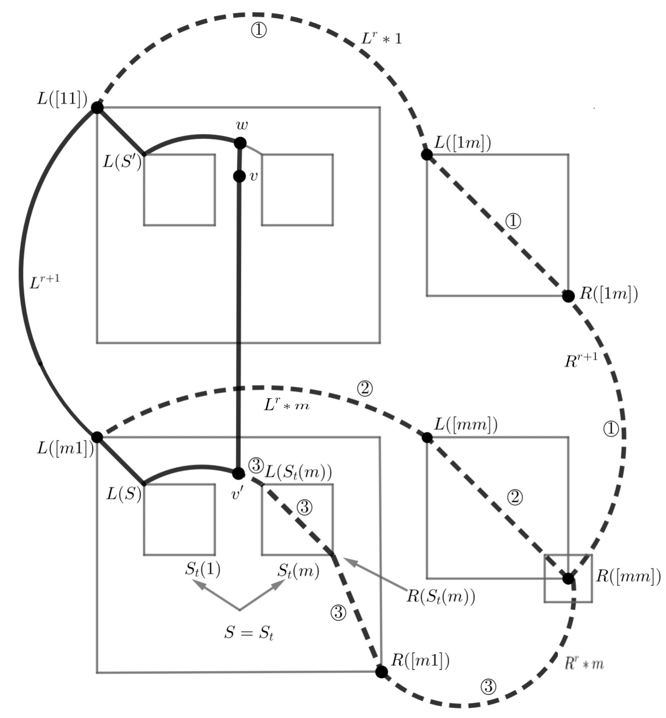
Since \(w\) corresponds to \(v'\) in \([1]\), then \(w\) belongs to a corresponding copy \(S''\) of \(S_{2}\subset [11]\). We then form a cycle \(T \subset S_{r+1}+vw\) (shown in bold in Figure 10) as follows,
\[T = v – w \xrightarrow{\:\text{$P_{L}(w)$ by Lc} \:} L(S'') \xrightarrow{\:\text{Lb} \:} L([11]) \xrightarrow{\:\text{$L^{r+1}$}\:} L([m1]) \xrightarrow{\:\text{Lb} \:} L(S') \xrightarrow{\:\text{Lc} \:} v' \xrightarrow{\:\text{$D(v',r+1)$} \:} v.\]
Observing that \(T\) does not enter \([mm]\), we can take \(R([mm])\notin T\), and obtain the following three independent \(R([mm]) – T\) paths (illustrated in dashed curves), where again paths numbered \(i\), \(1\le i\le 3\), in the figure correspond to paths \(P_{i}\) in the description which follows.
\[\begin{aligned}P_{1} =& R([mm]) \xrightarrow{\:\text{$R^{r}\ast m$} \:} R([m1]) \xrightarrow{\:\text{La} \:} R(S') \xrightarrow{\:\text{$P_{R}(v')$ by Lc} \:} q(v'), \,\,\, \text{(intersecting $T$ at $q(v')$)}, \\ P_{2} = &R([mm]) \xrightarrow{\:\text{Lb} \:} L([mm]) \xrightarrow{\:\text{$L^{r}\ast m$} \:} L([m1]),\,\,\, \text{(intersecting $T$ at $L([m1])$)},\\ P_{3} = &R([mm]) \xrightarrow{\:\text{$R^{r+1}$} \:} R([1m]) \xrightarrow{\:\text{Lb} \:} L([1m]) \xrightarrow{\:\text{$L^{r}\ast 1$} \:} L([11]),\,\,\, \text{(intersecting $T$ at $L([11])$)}.\end{aligned}\]
Still under the case \(v'\in SQ_{r+1}(m)\) suppose that \(v'\) is on some attachment path \(A = L^{t}\ast B\) in some copy \(S\) of \(S_{t}\subset S_{r+1}\), as illustrated in Figure 11. The reader can consult this figure as they read the analysis of this case.

Again we may suppose by symmetry that \(S\subset [m1]\) and that \(w\in S'\), where \(S'\) is the corresponding copy of \(S_{t}\) in \([11]\). Here \(w\) lies on the attachment path \(A' = L^{t}\ast B'\subset S'\) corresponding to \(A\) in \(S'\), where the tuples \(B\) and \(B'\) over \(\{m, 1\}\) differ only in their final letter, that being \(m\) in \(A\) and \(1\) in \(A'\). We have labeled the two subgraphs \(S_{t}(1)\) and \(S_{t}(m)\) of \(S\) in that figure. Note that \(L^{t}\ast B\) joins these two subgraphs at their left attachment points.
Now in \(S_{r+1}+vw\) we can form the cycle \(R\) and three independent \(R([mm])-R\) paths as follows, where know that \(R([mm])\notin R\) since \(R\) never enters \([mm]\).
\[\begin{aligned}R =& v – w \xrightarrow{\:\text{$L^{t}\ast B'$} \:} L(S') \xrightarrow{\:\text{La} \:} L([11]) \xrightarrow{\:\text{$L^{r+1}$} \:} L([m1]) \xrightarrow{\:\text{La} \:} L(S) \xrightarrow{\:\text{$L^{t}\ast B$} \:} v' \xrightarrow{\:\text{$D(v',r+1)$} \:} v,\\ P_{1} =& R([mm]) \xrightarrow{\:\text{$R^{r+1}$} \:} R([1m]) \xrightarrow{\:\text{Lb} \:} L([1m]) \xrightarrow{\:\text{$L^{r}\ast 1$} \:} L([11]),\,\,\, \text{(intersecting $R$ at $L([11])$)},\\ P_{2} =& R([mm]) \xrightarrow{\:\text{Lb} \:} L([mm]) \xrightarrow{\:\text{$L^{r}\ast m$} \:} L([m1]),\,\,\, \text{(intersecting $R$ at $L([m1])$)},\\ P_{3} =&R([mm]) \xrightarrow{\:\text{$R^{r}\ast m$} \:} R([m1]) \xrightarrow{\:\text{La} \:} R(S_{t}(m)) \xrightarrow{\:\text{Lb} \:} L(S_{t}(m)) \xrightarrow{\:\text{$L^{t}\ast B$} \:} v',\,\,\, \text{(intersecting $R$ at $v'$)} . \end{aligned}\]
This completes consideration of the case \(k = r+1\). The case \(k\le r\) is argued similarly, requiring several subcases. The missing edge \(vw\) is now no longer on a path in \(D(r+1)\). The cases involved still use the the decomposition of \(S_{r+1}\) into the subgraphs \([11], [1m], [m1, [mm]\) together with the various attachment paths and the connection paths in \(D(r)\) and \(D(r+1)\). In each case, we find an \(S(K_{4})\) in \(S_{r+1} + vw\) by finding a cycle \(C\), a point \(x\notin C\) and three independent \(x-C\) paths. We omit the arguments here, and instead provide the details in Appendix II. ◻
Proof. Since \(S_{r}\) is \(S(K_{4})\)-saturated by Theorems 4.3 and 4.10 it suffices to show that \(|E(S_{r})| = m^{r} + 2^{r-1} – 2\). We continue with the notation \([1]\) and \([m]\) from the preceding theorem.
For any connected graph \(G\) let \(f(G) = |E(G)| – |V(G)| +1\). We say that \(\mathcal{E}\subset E(G)\) is an excess set of \(G\) if \(G – \mathcal{E}\) is a spanning tree of \(G\), so that for such an \(\mathcal{E}\) we have \(|\mathcal{E}| = f(G)\). By Lemma 4.1 we know that \([D(r)]\) is a forest, each component tree of which is pendant on \(SQ_{r}\). So any edge of \([D(r)]\) is a cut edge of \(S_{r}\). Therefore for any excess set \(\mathcal{E}\) of \(S_{r}\) we have \(\mathcal{E}\cap [D(r)] = \emptyset\). So in fact \(\mathcal{E}\) must be an excess set of \(S_{r}\). So we let \(x_{r} = f(SQ_{r}) = f(S_{r})\), and we determine \(x_{r}\) from which we obtain \(|E(S_{r})| = x_{r} + m^{r} – 1\), since \(S_{r}\) is a connected spanning subgraph of \(P_{m}^{r}\).
Consider first \(x_{3}\). Now \(S_{3}(1)\cong S_{3}(m) = S_{2}\), and \(S_{2}\) contains a unique cycle (the outside cycle). Take the set \(\mathcal{E} = \{e_{1}, e_{2}, e_{3}\}\), where \(e_{1}\) (resp. \(e_{2}\)) is an edge on the unique cycle of \(S_{3}(1)\) (resp. \(S_{3}(m)\)), and \(e_{3}\) is any edge of \(L^{3}\cup R^{3}\), say of \(L^{3}\). Then we can see that \(SQ_{3} – \mathcal{E}\) is a spanning tree of \(SQ_{3}\) as follows. First note that \(SQ_{3} – \mathcal{E}\) spans \(V(S_{3})\). Since \(S_{3}(1)\) and \(S_{3}(m)\) are connected and unicyclic, then \(S_{3}(1) – e_{1}\) and \(S_{3}(m) – e_{2}\) are spanning trees of \(S_{3}(1)\) and \(S_{3}(m)\) respectively. Also \(R^{3}\) is a path joining these two spanning trees, thus yielding that \(SQ_{3} – \mathcal{E}\) is a spanning tree of \(SQ_{3}\). So \(\mathcal{E}\) is an excess set for \(SQ_{3}\), and hence \(x_{3} = 3\).
We claim that the sequence \(\{x_{r}: r\geq 3\}\) satisfies the recurrence \(x_{r+1} = 2x_{r} + 1\). For this, it suffices to find an excess set of \(SQ_{r+1}\) of size \(2x_{r} + 1\).
By construction we have \(SQ_{r+1} = (SQ_{r}\ast 1)\cup (SQ_{r}\ast m)\cup L^{r+1}\cup R^{r+1}\). Let \(\mathcal{E}_{1}\) (resp. \(\mathcal{E}_{2}\)) be an excess set in \(SQ_{r}\ast 1\) (resp. \(SQ_{r}\ast m\)) of size \(x_{r}\), and let \(e\) be any edge in \(L^{r+1}\cup R^{r+1}\). Letting \(\mathcal{E} = \mathcal{E}_{1}\cup \mathcal{E}_{2}\cup \{e\}\), we see that \(SQ_{r+1} – \mathcal{E}\) is a spanning tree of \(SQ_{r+1}\) as follows. This is because whichever of \(L^{r+1}\) or \(R^{r+1}\) that does not contain \(e_{3}\) is then a path in \(SQ_{r+1} – \mathcal{E}\) joining the two spanning trees \((SQ_{r}\ast 1) – \mathcal{E}_{1}\) and \((SQ_{r}\ast m) – \mathcal{E}_{2}\) of \(SQ_{r}\ast 1\) and \(SQ_{r}\ast m\) respectively. So \(\mathcal{E}\) is an excess set of \(SQ_{r+1}\), and has size \(x_{r+1} = 2x_{r} +1\), as required.
Finally a simple induction using this recurrence and \(x_{3} = 3\) shows that \(x_{r} = 2^{r-1} – 1\) is the unique solution to the recurrence for \(r\geq 3\). This yields \(|E(S_{r})| = m^{r} + 2^{r-1} – 2\) as required. ◻
In this paper we studied the saturation function \(Sat(P_{m}^{r}, S(K_{4}))\); that is, the minimum number of edges in any \(S(K_{4})\) saturated spanning subgraph of the \(r\)-dimensional grid \(P_{m}^{r}\). Here \(S(K_{4})\) is the graph family of all subdivisions of the complete graph \(K_{4}\). In dimension 2 we obtained the exact result \(Sat(P_{m}\times P_{n}, S(K_{4})) = mn + 1\) if at least one of \(m\) or \(n\) is odd with \(m\geq 5\) and \(n\geq 5\). In dimension 3 we found the near exact result \(m^{3} + 1 \le Sat(P_{m}^{3}, S(K_{4}))\le m^{3} + 2\) for \(m\) even with \(m\geq 4\). For arbitrary \(r\geq 3\) with \(m\) even and \(m\geq 4\), we proved that \(Sat(P_{m}^{r}, S(K_{4})) \le m^{r} + 2^{r-1} – 2\).
The upper bounds for dimension \(r\geq 3\) were obtained by the inductive construction of the \(S(K_{4})\)-saturated graph \(S_{r} \subseteq P_{m}^{r}\) described in the paper.
In this Appendix we prove independence of the three paths \(P_{1}, P_{2}, P_{3}\) used in the construction of an \(S(K_{4})\) in the proof of Theorem 4.10, in the case \(k = r+1\) and \(Source(w)\in [1m]\).
First we show that \(P_{1}\cap W = \{q(Source(v))\}\). The initial subpath of \(P_{1}\) satisfies \(W\cap \big{(}R([mm]) \xrightarrow{\:\text{$R^{r}\ast m$} \:} R([m1])\big{)} = \emptyset\). The remaining succession of paths on \(P_{1}\), which we call \(Q\), satisfies \(Q = R([m1]) \xrightarrow{\:\text{La} \:} R(S_{2}(Source(v))) \xrightarrow{\:\text{Ld} \:} q(Source(v))\) lies in \([m1]\). So it remains to show that \(Q\cap W\cap [m1] = \{q(Source(v))\}\). The subpath \(Q' = R([m1]) \xrightarrow{\:\text{La} \:} R(S_{2}(Source(v)))\) of \(Q\) is a right attachment path. But \(W\cap [m1]\) consists of a left attachment path (so it has empty intersection with \(Q'\)), a path in \(S_{2}(Source(v))\) avoiding \(R(S_{2}(Source(v)))\) (so having empty intersection with \(Q'\)), and finally a connection path \(Source(v) \xrightarrow{\: \text{L'b} \:} v\) which must have empty intersection with \(Q'\) since \(Q'\) contains no connection points and does not contain \(Source(v)\). We see that the subpath \(Q'' = R(S_{2}(Source(v))) \xrightarrow{\:\text{Ld} \:} q(Source(v))\) of \(Q\) lies in \(S_{2}(Source(v))\). But then Lemma 4.9c,d give that \(Q'' \cap (W\cap S_{2}(Source(v))) = \{q(Source(v))\}\). So we get \(Q\cap W\cap [m1] = \{q(Source(v))\}\) as desired.
Next we show that \(P_{2}\cap W = \{ L([m1])\}\). Since \(W\cap [mm] = \emptyset\), the initial subpath \(R([mm]) \xrightarrow{\:\text{Lb} \:} L([mm])\) of \(P_{2}\) has empty intersection with \(W\). The second subpath \(L([mm]) \xrightarrow{\:\text{$L^{r}\ast m$} \:} L([m1])\) of \(P_{2}\) intersects \(W\) at the vertex \(L([m1])\) by construction. Hence \(P_{2}\cap W = \{ L([m1])\}\) as required.
Now we show that \(P_{3}\cap W = \{q(Source(w))\}\). Here the proof is similar to the one given for showing \(P_{1}\cap W = \{q(Source(v))\}\). First observe that the initial subpath \(R([mm]) \xrightarrow{\:\text{$R^{r+1}$} \:} R([1m])\) has empty intersection with \(W\) by construction. The rest of \(P_{3}\) lies in \([1m]\), so it suffices to show that \(P_{3}\cap W\cap [1m] = \{q(Source(w))\}\). By construction \(W\cap [1m] = Source(w) \xrightarrow{\text{\: Lc \:}} L(S_{2}(Source(w))) \xrightarrow{\:\text{La} \:} L([10])\). Suppose first that \(Source(w)\ne L(S_{2}(Source(w)))\). Then the subpath. \(\lambda = L(S_{2}(Source(w))) \xrightarrow{\:\text{La} \:} L([1m])\) of \(W\cap [m1]\) has empty intersection with \(P_{3}\cap [1m]\), since \(\lambda\) is a left attachment path while \(P_{3}\cap [1m]\) is a right attachment path followed by a path \(R(S_{2}(Source(w))) \xrightarrow{\:\text{Ld} \:} q(Source(w))\) not containing \(L(S_{2}(Source(w)))\). It then remains to observe that the subpath \(Source(w) \xrightarrow{\text{\: Lc \:}} L(S_{2}(Source(w)))\) intersects the subpath \(R(S_{2}(Source(w))) \xrightarrow{\:\text{Ld} \:} q(Source(w))\) at \(q(Source(w))\) by Lemma 4.9c,d, showing that \(P_{3}\cap W\cap [1m] = \{q(Source(w))\}\) as desired. Now suppose that \(Source(w) = L(S_{2}(Source(w)))\). The we have \(Source(w) = q(Source(w))\). So the path \(R(S_{2}(Source(w))) \xrightarrow{\:\text{Ld} \:} q(Source(w))\) on \(P_{3}\) reaches \(L(S_{2}(Source(w))) = q(Source(w))\), and again we get \(P_{3}\cap W\cap [1m] = \{q(Source(w))\}\).
To complete the proof of independence of the three paths, we show that \(P_{1}\cap P_{2}\cap P_{3} = \{R([mm])\}\), where the containment \(R([mm])\in P_{1}\cap P_{2}\cap P_{3}\) is clear by definition. We easily have \(P_{3}\cap \big{(} P_{1}\cup P_{2} \big{)} = \{R([mm])\}\), since \(P_{1}\cup P_{2}\subset [m]\), while \(P_{3}\cap [m] = \{R([mm])\}\). As for \(P_{1}\cap P_{2}\), since \(P_{1}\cup P_{2}\subset [m]\) and since neither \(P_{1}\) nor \(P_{2}\) contain connection points of \([m]\), it suffices to show that \(P_{1}\cap P_{2}\cap [mm] = \{R([mm])\}\) and \(P_{1}\cap P_{2}\cap [m1] = \emptyset\). The first claim is clear since by definition \(P_{1}\cap [mm] = \{R([mm])\}\). For the second claim, we note that \(P_{2}\cap [m1] = \{L([m1])\}\). But \(P_{2}\cap [m1]\) is a right attachment path, which therefore cannot contain \(L([m1])\), followed by a path internal to \(S_{2}(Source(v))\) which avoids \(L(S_{2}(Source(v)))\) by Lemma 4.9d. So we obtain \(P_{1}\cap P_{2}\cap [m1] = \emptyset\), and it follows that \(P_{1}\cap P_{2}\cap P_{3} = \{R([mm])\}\), yielding the independence of the three paths \(P_{i}\), \(1\le i\le 3\).
In this Appendix we complete the proof of Theorem 4.10 by providing the details for the case \(k\le r\), where the nonedge \(vw\) being added to \(S_{r+1}\) has dimension \(k\) in \(P_{m}^{r+1}\). The case \(k = r+ 1\) in the proof of Theorem 4.10 was treated in the main body of the paper.
First we can reduce to the case where \(\{v,w\}\cap \big{(}[m]\cup [1]\big{)} = \emptyset\). Suppose not. If exactly one of \(v\) or \(w\) is in \([m]\cup [1]\), then \(vw\) is an \((r+1)\)-dimensional nonedge following or preceding some path \(D(v',r+1)\), a contradiction to \(k \le r\). If \(v\in [m]\) and \(w\in [1]\), then \(v_{r+1} = m\) and \(w_{r+1} = 1\), showing that \(v\) and \(w\) disagree (in fact by more than \(1\)) in the \((r+1)\)’st coordinate, so contradicting \(k \le r\). Finally with either \(\{v,w\}\subset [m]\) or \(\{v,w\}\subset [1]\), then induction immediately gives an \(S(K_{4})\) in either \([m]+vw\) or \([1]+vw\) and therefore in \(S_{r+1} + vw\), as required.
From \(\{v,w\}\cap \big{(}[m]\cup [1]\big{)} = \emptyset\) it follows from the decomposition of \(S_{r+1}\) at the beginning of the proof that \(\{v,w\}\subset D(r+1)\cup L^{r+1}\cup R^{r+1}\). We cannot have \(\{v,w\}\subset L^{r+1}\cup R^{r+1}\) since neither \(L^{r+1}\) nor \(R^{r+1}\) contain nonedges of \(P_{m}^{r+1}\), while points of \(L^{r+1}\) differ from points of \(R^{r+1}\) in more than one coordinate. Recalling the notation \(D'(r+1) = D(r+1) – \big{(}[1]\cup [m] \big{)}\) we must have either
both \(v\) and \(w\) in \([D'(r+1)]\), or
one of \(\{v,w\}\) in \(L^{r+1}\cup R^{r+1}\) while the other is in \([D'(r+1)]\).
We begin by assuming \(k = r\), and later consider the case \(k < r\).
Suppose first that \(v, w\in [D'(r+1)]\) as in case \((A)\), and we treat the case \((B)\) afterwards. Since \(k = r\), then \(v\) and \(w\) are on distinct \(D\)-paths in dimension \(r+1\), say \(v\in D(v',r+1)\) and \(w\in D(w',r+1)\), since otherwise \(v\) and \(w\) would disagree in coordinate \(r+1\), contrary to \(k = r\). By possibly renaming we can suppose \(v', w'\in [m]\). Now \(v\) (resp. \(w\)) disagrees with \(v'\) (resp. \(w'\)) only in the \((r+1)\)’st coordinate, but \(v\) and \(w\) disagree (by \(1\)) only in their \(r\)’th coordinate. Therefore \(v'\) and \(w'\) disagree by \(1\) only in the \(r\)’th coordinate. Then there are two possibilities under case \((A)\).
\(v'\) and \(w'\) are successive points on some \(D\)-path of dimension \(r\), or
\(v'\) and \(w'\) are successive points on the copy \(L^{r}\ast m\) of \(L^{r}\) or the copy \(R^{r}\ast m\) of \(R^{r}\) in \([m]\).
(resp. \(R^{r}\ast m\)) of \(L^{r}\) (resp. \(R^{r}\)) in \([m]\).
Consider first possibility case \((A1)\), shown in Figure 12. Then we can take \(v',w'\in D(u,r)\) with \(head(D(u,r)) = u\). So we must have \(u\in [m1]\cup [mm]\), and by symmetry we can take \(u\in [m1]\). So we have that \(v'\) and \(w'\) are in the same component of \([D(r+1)]\) as \(u\), so \(Source(w') = Source (v')\in [m1]\).
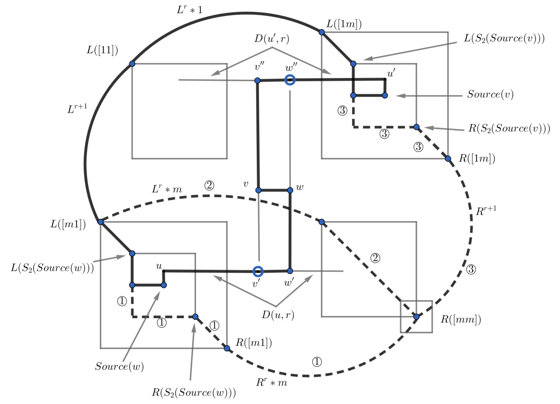
We claim that one of \(v',w'\) is the head of its \(D\)-path in dimension \(r+1\), while the other must be the tail of its \(D\)-path of this dimension, For this, note that \(v'\) and \(w'\) are neighbors in \(P_{m}^{r+1}\) so are on opposite sides of the bipartition of \(A_{r+1}, B_{r+1}\) in step \(5\) of the construction of \(S_{r+1}\). So by step \(6\) of that construction, \(v'\) and \(w'\) receive opposite head/tail designations for their \(D\)-paths dimension \(r+1\), proving the claim.
So arbitrarily take \(head(D(w',r+1)) = w'\), forcing \(tail(D(v',r+1)) = v'\). Therefore \(w\) is in the same tree component of \([D(r+1)]\) as \(w'\), so we get \(Source (w) = Source(w') = Source(v')\in [m1]\) since \(u\in [m1]\).
Now let \(v'' = head(D(v',r+1)\) and \(w'' = tail(D(w',r+1)\), so \(v'', w''\in [1]\). Then \(v''\) and \(w''\) are successive points on a path \(D(u',r)\subset [1]\), for some \(u'\in [1]\), corresponding to \(D(u,r)\subset [m]\). (We note here that in possibility (2), \(v''\) and \(w''\) are successive points on either \(L^{r}\ast 1\) or \(R^{r}\ast 1\), which will be considered when \((2)\) is analyzed.) Since \(D(u,r)\) and \(D(u',r)\), together with their heads and tails, are corresponding \(D\)-paths of dimension \(r\) in \([m]\) and \([1]\) respectively, we have \(D(u',r) = D(u,r)^{R}\) by step \(7\) of the construction of \(S_{r+1}\). So the point \(z\in D(u',r)\) corresponding to \(u\) is \(tail(D(u',r))\), noting also that \(z\in [11]\). Hence \(head(D(u',r))\in [1m]\), and by renaming we can let \(u' = head(D(u',r))\in [1m]\). So \(Source(w'') = Source(v'') = Source(v)\in [1m]\) and still recall that \(Source(w)\in [m1]\). The various \(D\)-paths and points are illustrated in Figure 12.
We now form the cycle \(W'\) in \(S_{r+1} + vw\) as follows.
\[\begin{aligned}W' =& w – v \xrightarrow{\:\text{L'b} \:} Source(v) \xrightarrow{\:\text{$P_{L}(Source(v))$ by Lc} \:} L(S_{2}(Source(v))) \xrightarrow{\:\text{La} \:} L([1m]) \xrightarrow{\:\text{$L^{r}\ast 1$} \:} L([11]) \xrightarrow{\:\text{$L^{r+1}$}}\\ &L([m1]) \xrightarrow{\:\text{La} \:} L(S_{2}(Source(w))) \xrightarrow{\:\text{$P_{L}(Source(w))$ by Lc} \:} Source(w) \xrightarrow{\:\text{L'b} \:} w.\end{aligned}\]
We then take \(R([mm])\notin W'\), and form the three independent \(R([mm])-W'\) paths in \(S_{r+1} + vw\) as follows.
\[\begin{aligned}P_{1} =& R([mm]) \xrightarrow{\:\text{$R^{r}\ast m$}} R([m1]) \xrightarrow{\:\text{La} \:} R(S_{2}(Source(w))) \xrightarrow{\:\text{Ld} \:} q(Source(w)),\\ &\text{(intersecting $W'$ at $q(Source(w))$)},\\ P_{2} =& R([mm]) \xrightarrow{\:\text{Lb} \:} L([mm]) \xrightarrow{\:\text{$L^{r}\ast m$}} L([m1]),\,\,\,\text{(intersecting $W'$ at $L([m1])$)},\\ P_{3} =& R([mm]) \xrightarrow{\:\text{$R^{r+1}$}\:} R([1m]) \xrightarrow{\:\text{La} \:} R(S_{2}(Source(v))) \xrightarrow{\:\text{Ld} \:} q(Source(v)),\\ &\text{(intersecting $W'$ at $q(Source(v))$)}.\end{aligned}\]
Consider now possibility case \((A2)\), still in case \(A\) and with \(k = r\). Here \(v'\) and \(w'\) are successive points on \(L^{r}\ast m\) or on \(R^{r}\ast m\), say by symmetry on \(R^{r}\ast m\). So \(v''\) and \(w''\) are corresponding successive points on \(R^{r}\ast 1\). As before we can take \(w' = head(D(w',r+1))\) and \(v' = tail(D(v',r+1))\). This case is illustrated in Figure 13.
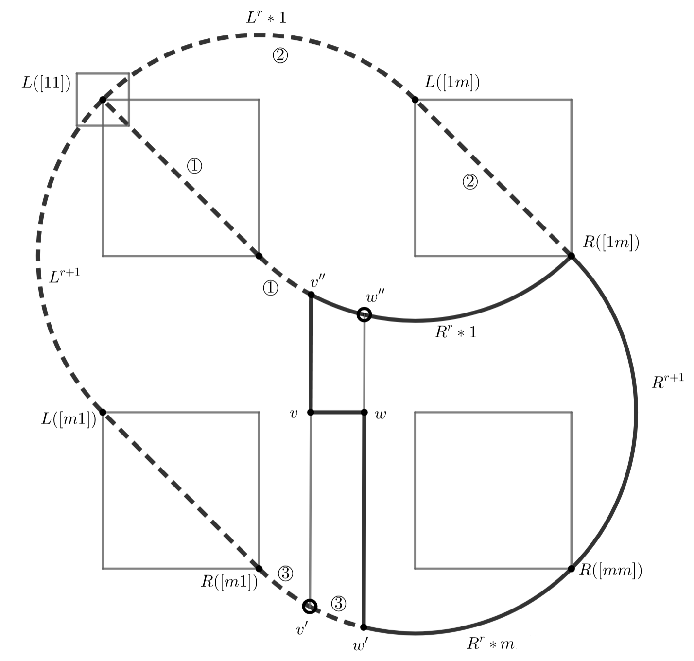
First we form the cycle \(W''\), indicated in bold in that figure, as follows.
\[W'' = w – v \xrightarrow{\:\text{$D(v'',r+1)$} \:} v'' \xrightarrow{\:\text{$R^{r}\ast 1$} \:} R([1m]) \xrightarrow{\:\text{$R^{r+1}$} \:} R([mm]) \xrightarrow{\:\text{$R^{r}\ast m$} \:} w'\xrightarrow{\:\text{$D(w',r+1)$} \:} w.\]
Now we take \(L([11])\notin W''\), and form three independent \(L([11]) – W''\) paths as follows. \[\begin{aligned}P_{1} =& L([11]) \xrightarrow{\:\text{Lb} \:} R([11]) \xrightarrow{\:\text{$R^{r}\ast 1$} \:} v'',\,\,\, \text{(intersecting $W''$ at $v''$)},\\ P_{2} = &L([11]) \xrightarrow{\:\text{$L^{r}\ast 1$} \:} L([1m]) \xrightarrow{\:\text{Lb} \:} R([1m]),\,\,\, \text{(intersecting $W''$ at $R([1m])$)},\\ P_{3} =& L([11]) \xrightarrow{\:\text{$L^{r+1}$} \:} L([m1]) \xrightarrow{\:\text{Lb} \:} R([m1]) \xrightarrow{\:\text{$R^{r}\ast m$} \:} w' ,\,\,\, \text{(intersecting $W''$ at $w''$)}.\end{aligned}\]
Still assuming \(k = r\), consider case \((B)\); that is, where one of \(v,w\) is in \(L^{r+1}\cup R^{r+1}\) while the other is in \([D'(r+1)]\) and illustrated in Figure 14. By symmetry we can suppose \(v\in L^{r+1}\), the latter having endpoints \(L([11])\) and \(L([m1])\), the case \(v\in R^{r+1}\) being essentially the same. Now \(w\in D(w', r+1)\) where \(w'\in [m]\cup [1]\), and by symmetry we take \(w'\in [m]\).
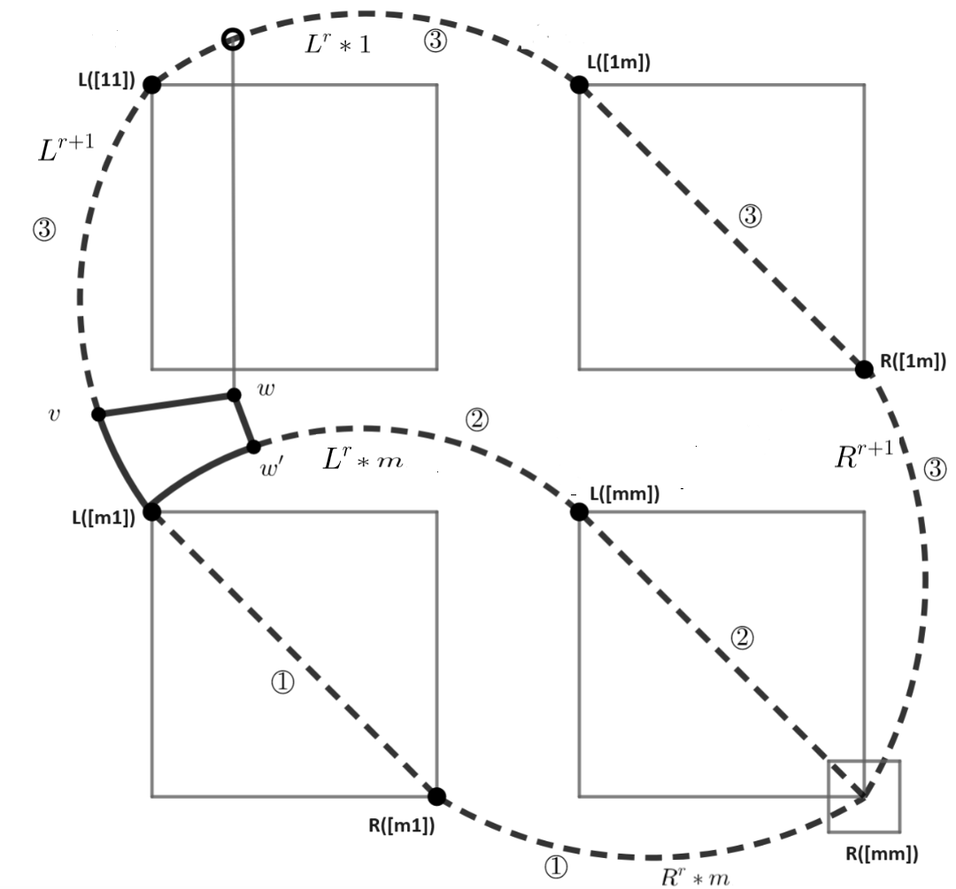
We can further specify \(w'\) as follows. Now \(k = r\) implies \(w_{r+1} = v_{r+1}\) and \(|w_{r} – v_{r}| = 1\). Since \(v_{r} = L([m1])_{r}\) and \(w_{r}' = w_{r}\), we then obtain \(|w_{r}' – L([m1])_{r}| = 1\). So this forces \(w'\) to be the point on \(L^{r}\ast m\) adjacent to \(L([m1])\).
Since \(L([11])\in A_{r+1}\), then \(L([m1])\in B_{r+1}\) because \(m\) is even. Hence \(w'\in A_{r+1}\), so by construction \(w' = head(D(w', r+1))\). Then in \(S_{r+1} +vw\) we have have a cycle \(Y\), the point \(R([mm])\notin Y\), and three independent \(R([mm]) – Y\) paths \(P_{i}\), \(1\le i\le 3\), as follows. In Figure 14, \(Y\) is the \(4\)-cycle illustrated in bold lines, and the paths \(P_{i}\) in dashed lines. \[\begin{aligned}Y =& w – v \xrightarrow{\:\text{$L^{r+1}$ } \:} L([m1]) \xrightarrow{\:\text{$L^{r}\ast m$} \:} w' \xrightarrow{\:\text{$D(w', r+1)$} \:} w,\\ P_{1} = &R([mm]) \xrightarrow{\:\text{$R^{r}\ast m$} \:} R([m1]) \xrightarrow{\:\text{Lb} \:} L([m1]),\,\,\, \text{(intersecting $Y$ at $L([m1])$)},\\ P_{2} =& R([mm]) \xrightarrow{\:\text{Lb} \:} L([mm]) \xrightarrow{\:\text{$L^{r}\ast m$} \:} w',\,\,\, \text{(intersecting $Y$ at $w'$)},\\ P_{3} = &R([mm]) \xrightarrow{\:\text{$R^{r+1}$} \:} R([1m]) \xrightarrow{\:\text{Lb} \:} L({1m}) \xrightarrow{\:\text{$L^{r}\ast 1$} \:} L([11]) \xrightarrow{\:\text{$L^{r+1}$} \:} v,\,\,\, \text{(intersecting $Y$ at $v$)}.\end{aligned}\]
This completes the analysis of the possibility \(k = r\), and we now move to the assumption \(k < r\). Again we begin with case \((A)\), where \(v,w\in [D'(r+1)]\). Figure 15 illustrates this case. The labeled vertices in this figure are explained in the discussion which follows, and the reader may wish to follow this discussion using the figure for illustration.
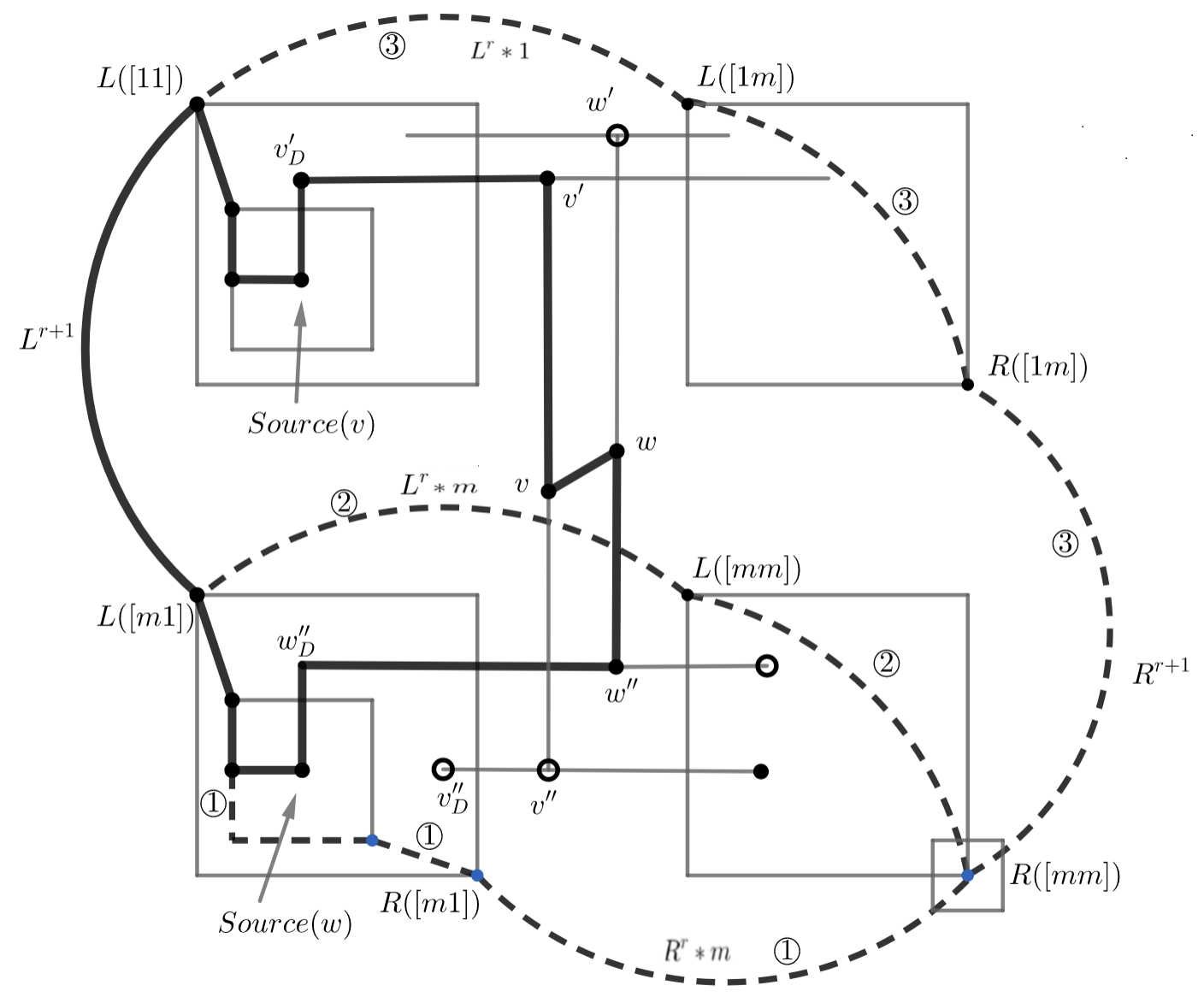
Let \(v', w'\in [1]\) correspond to \(v\) and \(w\) in \([1]\); that is, \(v'_{r+1} = w'_{r+1} = 1\) while \(v'_{j} = v_{j}\) and \(w'_{j} = w_{j}\) for \(1\le j\le r\). Similarly let \(v'', w''\in [m]\) be such that \(v''_{r+1} = w''_{r+1} = m\) while \(v''_{j} = v_{j}\) and \(w''_{j} = w_{j}\) for \(1\le j\le r\). Since \(v''_{r} = v_{r} = w_{r} = w''_{r}\), we see that \(v''\) and \(w''\) are on distinct \(D\)-paths of dimension \(r\) in \([m]\), while \(v'\) and \(w'\) are on the corresponding distinct \(D\)-paths of dimension \(r\) in \([1]\). Now \(v'\) and \(w'\) are neighbors in \(P_{m}^{r+1}\), so are on opposite sides of the bipartition \(A_{r+1}, B_{r+1}\) of \(P_{m}^{r+1}\). So \(v'\) and \(w'\) receive opposite head/tail designations in \(D(v',r+1)\) and \(D(w',r+1)\) respectively. By symmetry we can take \(v' = head(D(v',r+1))\) so \(w' = tail(D(w',r+1))\), so \(v'\in A_{r+1}\) and \(w'\in B_{r+1}\). Therefore \(v'' = tail(D(v',r+1))\) and \(w'' = head(D(w',r+1))\) and \(v''\) and \(w''\) are neighbors in \(P_{m}^{r+1}\) with \(v''\in B_{r+1}\) and \(w''\in A_{r+1}\).
Now let \(w''_{D}\in [m1]\) be the vertex with \((w''_{D})_{r} = 1\) and \((w''_{D})_{j} = w''_{j}\) for \(j\ne r\). Similarly let \(v''_{D}\in [m1]\) (resp. \(v'_{D}\in [11]\)) be such that \((v''_{D})_{r} = 1\) and \((v''_{D})_{j} = v''_{j}\) for \(j\ne r\) (resp. \((v'_{D})_{r} = 1\) and \((v''_{D})_{j} = v'_{j}\) for \(j\ne r\)). So we have \(w''\in D(w''_{D}, r)\), and by symmetry we can take \(w''_{D} = head(D(w''_{D}, r))\). So we have \(Source(w) = Source(w'')\in [m1]\). Again, the situation is illustrated in Figure 15.
We claim that \(Source(v)\in [11]\). For this it suffices to show that \(Source(v')\in [11]\) since \(v\) and \(v'\) are joined by a path (in fact he subpath subpath \(v\cdots v'\) of \(D(v'', r)\)) in \(D(r+1)\). Since \(v''_{r} = w''_{r}\) we have \(dist_{S_{r+1}}(v'', v''_{D}) = dist_{S_{r+1}}(w'', w''_{D})\). So since \(v''\) and \(w''\) are on opposite sides of the bipartition \((A_{r+1}, B_{r+1})\), it follows that \(v''_{D}\) and \(w''_{D}\) are also on opposite sides of the same bipartition. So we get \(v''_{D} = tail(D(v''_{D}, r))\) since \(w''_{D} = head(D(w''_{D}, r))\). But since \(D(v''_{D}, r) = D(v'_{D}, r)^{R}\) by construction, we get \(v'_{D} = head(D(v'_{D}, r))\). It follows that \(Source(v') = Source(v'_{D})\in [11]\), so finally \(Source(v)\in [11]\). Again see Figure 15.
We can then form our cycle \(C\) (shown in bold in Figure 15 ) and point \(R([mm])\notin C\), together with three independent \(R[mm] – C\) paths (shown dashed in that figure) as follows. \[\begin{aligned}C =& w – v \xrightarrow{\:\text{$D(v', r+1)$ } \:} v' \xrightarrow{\:\text{path through $v_{D}'$ } \:} Source(v) \xrightarrow{\:\text{$P_{L}(Source(v))$} \:} L(S_{2}(Source(v))) \xrightarrow{\:\text{La}}\\& L([11]) \xrightarrow{\:\text{$L^{r+1}$} \:} L([m1]) \xrightarrow{\:\text{La}} L(S_{2}(Source(w))) \xrightarrow{\:\text{$P_{L}(Source(w))$} \:}\\& Source(w) \xrightarrow{\:\text{path through $w_{D}'', w''$} \:} w,\\ P_{1} =& R([mm]) \xrightarrow{\:\text{$R^{r}\ast m$}} R([m1]) \xrightarrow{\:\text{La} \:} R(S_{2}(Source(w))) \xrightarrow{\:\text{Ld} \:} q(Source(w)),\\ &\text{(intersecting $C$ at $q(Source(w))$)},\\ P_{2} =& R([mm]) \xrightarrow{\:\text{Lb} \:} L([mm]) \xrightarrow{\:\text{$L^{r}\ast m$}} L([m1]),\,\,\, \text{(intersecting $C$ at $L([m1])$)},\\ P_{3} =& R([mm]) \xrightarrow{\:\text{$R^{r+1}$}} R([1m]) \xrightarrow{\:\text{Lb} \:} L([1m]) \xrightarrow{\:\text{$L^{r}\ast 1$} \:} L([11]),\,\,\, \text{(intersecting $C$ at $L([11])$)}.\end{aligned}\]
Still with \(k < r\), we finally consider case \((B)\), where one of \(\{ v,w \}\) is in \(L^{r+1}\cup R^{r+1}\) while the other is in \([D'(r+1)]\). One of the subcases here described later is illustrated in Figure 16. That figure is still useful for the reductions which follow.
By symmetry we can take \(v\in L^{r+1}\), recalling that the path \(L^{r+1}\) has ends \(L([m1])\) and \(L([11])\). Also \(w = D(w', r+1)\) where we can take \(w'\in [m]\) or \(w'\in [1]\), and we can arbitrarily take \(w'\in [m]\). With the same argument as in the case \(k = r\), we find that \(w'\) must be a neighbor in \(P_{m}^{r+1}\) of \(L([m1])\) across an edge of dimension \(k\). A straightforward induction on \(r\) shows that \(deg_{P_{m}^{r+1}}(x) = deg_{S_{r+1}}(x) = r+1\) for \(x\in \{ L([11]), L([1m]), L([m1]), L([mm]) \}\). Hence \(w'\) is a neighbor of \(L([m1])\) in \(S_{r+1}\). Observe further that every neighbor of \(L([m1])\) in \(S_{r+1}\) across an edge of dimension \(k\geq 3\) lies on some left attachment path \(L^{k}\ast B\) for some length \(r+1-k\) string \(B\) over \(\{m,1\}\), while for dimension \(k = 1,2\) the two neighbors of \(L([m1])\) are in the square \(S_{2}(L([m1]))\) containing \(L([m1])\).
We are therefore reduced to the following two cases defined by \(w'\):
\(w'\) is the point adjacent to \(L([m1])\) on some attachment path \(L^{k}\ast B\), or
\(w'\) belongs to no attachment path, in which case \(w'\) is one of the two neighbors of \(L([m1])\) in \(S_{2}(L([m1]))\).
Consider first case a), illustrated in Figure 16 with details which follow. Then \(L^{k}\ast B\) is in a subgraph \(S = S_{k}\ast B\subset [m1]\). In Figure 16 we illustrate the subgraphs \(S(1)\) and \(S(m)\) by two smaller rectangles inside the lower left larger rectangle representing \([m1]\). The ends of the attachment path \(L^{k}\ast B\) are shown as \(L([m1])\) and \(F\), while the ends of \(R^{k}\ast B\) as \(G\) and \(R(S) = H\). (Though we don’t use this in the construction which follows, we can deduce \(B\) by observing that every vertex in \(S\) has the same \(r+1-k\) length suffix \(B\) as \(L([m1])\), so \(B = 1^{r-k}m\). From this and \(L([m1]) = 1^{r}m\) we can deduce the coordinates \(F = 1^{k-1}m1^{r-k}m\), \(G = m^{k-1}1\ast 1^{r-k}m\) and \(R(S) = m^{k}\ast 1^{r-k}m\).)
We now have in \(S_{r+1}+vw\) the cycle \(C'\), the point \(R(S)\notin C'\), and three independent \(R(S) – C'\) paths \(R_{i}\) as follows and illustrated in the Figure 16.
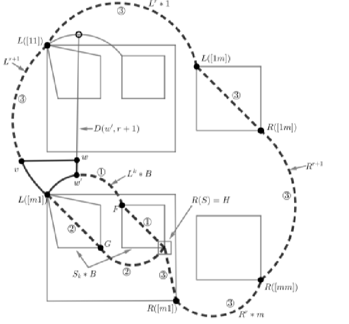
\[\begin{aligned}C' =& w – v \xrightarrow{\:\text{$L^{r+1}$} \:} L([m1]) \xrightarrow{\:\text{$L^{k}\ast B$} \:} w' \xrightarrow{\:\text{$D(w', r+1)$} \:} w,\\ R_{1} =& R(S) \xrightarrow{\:\text{$Lb$} \:} F \xrightarrow{\:\text{$L^{k}\ast B$} \:} w',\,\,\, \text{(intersecting $C'$ at $w'$)},\\ R_{2} =& R(S) \xrightarrow{\:\text{$R^{k}\ast B$}\:} G \xrightarrow{\:\text{$Lb$} \:} L([m1]),\,\,\, \text{(intersecting $C'$ at $L([m1])$),}\\ R_{3} =& R(S) \xrightarrow{\:\text{$La$} \:} R([m1]) \xrightarrow{\:\text{$R^{r}\ast m$} \:} R([mm]) \xrightarrow{\:\text{$R^{r+1}$} \:} R([1m]) \xrightarrow{\:\text{$Lb$} \:} L([1m])\xrightarrow{\:\text{$L^{r}\ast 1 $} \:} L([11]) \xrightarrow{\:\text{$L^{r+1}$} \:} v,\\ &\text{(intersecting $C'$ at $v$).}\end{aligned}\]
Now consider the second case b); that is, where \(w'\) belongs to no attachment path and is adjacent to \(L([m1])\) in \(S_{2}(L([m1]))\). Observe here that \(w' = head(D(w', r+1))\). This is because \(L([11]) = 1^{r+1}\in A_{r+1}\), so \(L([m1])\in B_{r+1}\) (since \(m\) is even), so \(w'\in A_{r+1}\cap [m]\) since \(w'\) is a neighbor of \(L([m1])\). Now in \(S_{r+1} +vw\) we form a cycle \(C''\), the point \(R([mm])\notin C''\), and three independent \(R([mm]) – C''\) paths \(Q_{i}\) as follows. \[\begin{aligned}C'' =& w – v \xrightarrow{\:\text{$L^{r+1}$} \:} L([m1]) \xrightarrow{\:\text{edge in $S_{2}(L([m1]))$ } \:} w' \xrightarrow{\:\text{$D(w', r+1)$} \:} w,\\ Q_{1} =& R([mm]) \xrightarrow{\:\text{Lb} \:} L([mm]) \xrightarrow{\:\text{$L^{r}\ast m$} \:} L([m1]),\,\,\, \text{(intersecting $C''$ at $L([m1])$)},\\ Q_{2} =& R([mm]) \xrightarrow{\:\text{$R^{r}\ast m$} \:} R([m1]) \xrightarrow{\:\text{Lb} \:} R(S_{2}(w')) \xrightarrow{\:\text{path in $S_{2}(w')$ } \:} w' ,\,\,\, \text{(intersecting $C''$ at $w'$)},\\ Q_{3} =& R([mm]) \xrightarrow{\:\text{$R^{r+1}$} \:} R([1m]) \xrightarrow{\:\text{Lb} \:} L([1m]) \xrightarrow{\:\text{$L^{r}\ast 1$} \:} L([11]) \xrightarrow{\:\text{$L^{r+1}$} \:} v,\,\,\, \text{(intersecting $C''$ at $v$)}.\end{aligned}\]