
In recent years, food safety and quality and safety accidents have occurred frequently, including the production of food raw materials, food processing, food packaging and product storage and transportation of the whole process there are many quality and safety problems [9, 15]. Food safety industry quality and safety management in a serious form, the application of information technology to establish food quality and safety management system, to complete the food gatekeeper, traceability, set limits and control and other aspects of management, to enhance the industry supervision work is of great significance.
With the continuous development of science and technology, image recognition technology is more and more widely used in the field of food safety inspection. The national supervision department attaches great importance to the quality of food production, the supervision is more and more strong, through the image recognition and other means of supervision, not only improves the efficiency and accuracy of food safety detection, but also makes the food quality and safety management has been effectively improved [8,12,10]. Image recognition technology is to collect, process and analyze the images of food by computer, so as to detect the packaging material, food appearance information, internal structure texture, ingredient content and freshness of food [4,3, 13]. And the abnormal pattern of image recognition is mainly through machine learning and deep learning and other technologies, a large number of food image data for training and learning, to establish a classification model of the abnormal pattern of food, through the model of the food images to be tested to analyze and identify, to determine whether there is anomalies in the food [20, 6, 17,19]. However, in the process of practical application, the accuracy of food safety detection may be affected by a variety of factors, such as environmental changes, diversity of food types and sample variability [14]. Therefore, in order to improve the accuracy of image recognition food safety detection, continuous learning and optimization of the model is required. This usually includes operations such as updating the parameters of the model, introducing new training samples and adjusting the model’s architecture [2,7]. Such an image recognition anomaly model has the advantages of high efficiency, high accuracy, non-destructiveness and comprehensiveness in food safety detection [5,21]. The anomaly pattern recognition method based on image recognition has important application value in food safety detection.
In this paper, in order to improve the real-time and accuracy of foreign object judgment and recognition, fuzzy recognition technology is used to identify the types of foreign objects in food images formed by X-ray irradiation. Firstly, bilateral filtering is used to remove the noise in the original food graphic, and contrast stretching transformation method is utilized to enhance the denoised X-ray image. Then from the perspective of mathematical morphology, the threshold segmentation technique is used to segment the food graphics effectively. Finally, combined with the BP neural network algorithm, the graphical features of food foreign objects are extracted to realize the safety detection of food foreign objects based on X-ray. The performance of the designed algorithm is verified on the data and and its practical application effect is analyzed.
This system can be realized in the following two ways:
DSP + FPGA image processing and foreign object recognition system.
The use of DSP combined with FPGA to process images, mainly using the logic processing capabilities of FPGA to carry out the front-end preprocessing of images, the use of high-performance DSP as the core CPU for image processing, DSP internal resources are very rich, used for the implementation of image processing algorithms have unique advantages for real-time processing can play a great help. However, the development of this program involves the development of hardware circuits, and software programming is very cumbersome, the development of a large cycle is long and very complex.
Computer software image processing and foreign object recognition system.
This program takes full advantage of the simplicity of computer programming, although the real-time is not as good as the previous one, but basically to meet the actual needs of the development cycle is short, do not have to design too much knowledge of the hardware, so this program is used.
Image acquisition card is the interface between the image acquisition part and the image processing part. The process in which an image is sampled, quantized, converted to a digital image, input and stored in the frame memory is called acquisition. Since the transmission of image signals requires high transmission speeds, general-purpose transmission interfaces can not meet the requirements, so the need for image acquisition card. Image acquisition card also provides the function of digital IO. After the trigger signal is generated by the external optical trigger sensor or the system software, a frame of the selected length (i.e., number of lines) is captured, processed, transmitted and stored in the capture card memory. However, a very important feature of the \(X\)-ray detector chosen for this system is that the image frame size and the start and end of the frame functions are only available within the frame grabber card. Once the operating parameters have been set, the \(X\)-ray detector produces image data continuously, line by line, completely independently of the acquisition card, which no longer has any logical control over it. Even when the acquisition card is completely stopped or the \(X\)-ray beam is turned off, the \(X\)-ray detector still produces image data line by line. The user interface software provides complete control over when and how the acquisition card receives the image data and how the data is further processed.
The Image Acquisition Card acquires the 16-bit parallel digital image data from the \(X\)-ray detector via an RS422 standard interface. In addition to the actual data signal, there is a 4-bit control signal at the image acquisition card interface. The image acquisition card uses the PCI slot on the motherboard of the industrial control computer and communicates with the main control computer via the PCI bus.
This system uses Coreco PC-DIG image acquisition card, the image acquisition module calls the driver and dynamic link library provided by the image acquisition card manufacturer. The image is transferred to the host computer’s memory at a speed of 120MB/sec, and images can be captured from digital cameras or sensors in 8, 10, or 12-bit LVDS or RS-422 format, with a pixel clock of up to 40MHz.
Driven by a conveyor belt, the food slowly passes through the \(X\)-ray detection system and is scanned line by line. The scintillation crystal screen inside the line array detector firstly transforms \(X\) rays into visible light, and then through photoelectric conversion, generates charges in each detection unit and accumulates them continuously. The line array detector starts the digital image acquisition process through the timed reading operation, and except for the instantaneous process of image reading out, each detection unit accumulates the light charges continuously. In the image readout process, the charge is transmitted line by line from the capacitance of each detection unit, the charge from each detection unit is corrected and written into a first-in-first-out queue to go, in the queue of data through the data connector to the RS422 format to the computer processing system to go.
The data transmitted by the acquisition card is line data, in this system 1 * 1024 size data, this data to do image processing is very inconvenient, and can not be based on this line of images to determine the characteristics of the foreign body, so you need to line data splicing, to get the whole image containing the food as a whole.
This can be done in two ways:
1) Because the food passes through the detection area on the conveyor belt at a certain speed, it can be controlled to stitch the data collected during the formulated time into one image, which is inversely proportional to the speed of the conveyor belt and directly proportional to the size of the food. i.e., \[\label{GrindEQ__1_} t=C\frac{l}{v} ,\tag{1}\] where \(C\) is a constant and 1 and \(v\) are the food size and conveyor speed respectively. The spliced image of this method generally meets the requirements, but sometimes the spacing of the food on the conveyor belt is not exactly the same, so sometimes the spliced image will lose part of the data, so it can be seen that this method needs to be improved.
2) The conveyor belt drives the food through the \(X\)-ray detection area, because the conveyor belt is generally more uniform thickness, so the conveyor belt is \(X\)-ray scanning rows of data after the image is not much difference in grayscale, so you can set a threshold to detect the difference in grayscale of the collected rows of data, and if greater than this threshold is considered to have detected the foodstuffs, and then a certain period of time of the rows of data spliced together into a single image, and then the image is processed [11].
Before acquiring the \(X\)-ray images, the boxed frozen foods were divided into two groups, \(A\) and \(B\), and melted at room temperature, and when the foods were fluffy, scissors and tweezers were used to put the foreign objects inside the foods in group \(B\). In order to maximize the image contrast and minimize the image noise, 10 sets of tested \(X\)-ray food images were used to adjust the \(X\)-ray tube voltage and tube current parameters, and the optimal tube voltage range of 60\(\mathrm{\sim}\)80 kv and tube current of 0.8\(\mathrm{\sim}\)1 mA were finally obtained.After setting the optimal parameters, 300 \(X\)-ray images of foreign body-free food and 300 \(X\)-ray images of foreign body-free food were acquired, respectively.
Distribution characteristics of different foreign objects in \(X\)-ray images.
Metals: Because of their high density and poor penetrability, metal steel balls, screws and wires show a distribution characteristic of low gray scale, dark color, large difference and sharp contrast with the surrounding objects and background in \(X\)-ray food images.
Stones: Stones are slightly less dense and less penetrating than metallic foreign objects, but much denser than foodstuffs, so they are able to present clear outlines and gray values different from those of foodstuffs in \(X\)-ray irradiation.
Glass: Transparent glass has a lower density than metal and stone, but good penetrability, and in \(X\)-ray images, presents a gray scale similar to that of food, with poor contrast, which is confusing and not easy to recognize.
Sources of noise in \(X\)-ray food images.
\(X\) Noise in ray food images is caused by a combination of natural conditions at the time of the experiment, such as light, as well as many factors such as the instrument’s circuitry, signal transmission, and A/D conversion. They are categorized as follows according to the specific conditions:
Noise inside the \(X\)-ray generator due to electronic ups and downs, or noise due to slightly different wavelengths of excited \(X\)-rays due to unstable tube voltage or tube current.
\(X\)-ray scattering, reflection of the photon noise generated, etc..
The detection environment is interfered by external electromagnetic waves, such as antenna interference.
Electronic noise generated by internal electronic devices such as image detectors, including AD conversion noise, D/A conversion noise, image element noise, etc.
Noise generated by mechanical movement. Due to voltage and current instability leads to image acquisition and processor device jitter, such as storage disk head jitter occurs.
Image denoising is the process of reducing noise in a digital image while preserving as many detailed features of the image as possible. The ultimate goal of denoising is to improve a given image and solve the problem of degradation of image quality due to noise interference in the actual image. Denoising techniques can effectively improve the quality of the image, increase the signal-to-noise ratio, and better reflect the information carried by the original image. Frequently used image denoising methods include mean filtering, median filtering, bilateral filtering and non-local mean filtering.
Bilateral filter is a kind of nonlinear filter, which mainly combines spatial information and brightness similarity to the image filtering process, while smoothing the image can be retained at the same time the edges and details of the image features [18]. Bilateral filters consider not only the effect of position on the center pixel, but also the effect of the similarity between the pixels in the convolution kernel and the center pixel, so that in bilateral filters, the value of the output pixel depends on the weighted combination of the neighboring pixel values, defined as follows: \[\label{GrindEQ__2_} g(i,j)=\frac{\sum\limits_{(x,y)\in R}f (x,y)\omega (i,j,x,y)}{\sum\limits_{(x,y)=\Omega }\omega (i,j,x,y)} ,\tag{2}\] where \(g(i,j)\) is the output image, \(f(x,y)\) is the input image, \(\Omega\) a domain window centered at pixel \((x,y)\), and the filter kernel \(\omega (i,j,x,y)\) depends on the product of the null domain kernel \(\phi\) and the value domain kernel \(\psi\). Both filter kernels are usually in the form of Gaussian functions, i.e.: \[\label{GrindEQ__3_} \phi (i,j,x,y)=\exp \left(-\frac{(i-x)^{2} +(j-y)^{2} }{2\sigma _{d}^{2} } \right),\tag{3}\] \[\label{GrindEQ__4_} \psi (i,j,x,y)=\exp \left(-\frac{\left\| f(i,j)-f(x,y)\right\| ^{2} }{2\sigma _{r}^{2} } \right),\tag{4}\] where \(\sigma _{d}\) is the standard deviation of the null domain Gaussian function and \(\sigma _{r}\) is the standard deviation of the value domain Gaussian function. From the above equation, it can be seen that the null domain filter coefficients depend on the spatial distance between pixels, the smaller the distance, the larger the value. The value domain filter coefficients depend on the similarity between pixels, the closer the pixels are, the larger the coefficients are. In the region of smooth gray scale change, the value domain filter coefficient is close to 1, then the null domain filter plays the main role, and the bilateral filter degrades to a Gaussian low-pass filter, which smoothes the image. In the region where the image changes sharply (the edge of the image), the difference between pixels is large, and the value domain filtering plays a major role, so that the image edge information can be maintained.
Image enhancement is an image processing method that makes the original unclear image clear or emphasizes certain features of interest in the image and suppresses the uninteresting features, so as to improve the image quality, enhance the image contrast, enrich the amount of information in the image, and strengthen the effect of image interpretation and recognition. When using \(X\)-ray imaging system to collect food images, due to the small dynamic range of the flat panel detector and underexposure or overexposure and other reasons, the acquired food images have insufficient contrast, unclear details and other problems, so it is necessary to carry out the image enhancement process to improve the visual effect of the image, so as to facilitate the analysis of the image in the later stage of the calculation and identification. Image enhancement techniques can be categorized into two main categories, namely, enhancement algorithms based on the null domain and enhancement algorithms based on the frequency domain, according to the different processing spaces. The former directly calculates the gray value of the image during processing, mainly gray scale transformation, histogram method, etc. The latter is to correct the transformation coefficients of the image in some kind of transform domain of the image, which is an indirect image enhancement algorithm, mainly frequency domain filtering, homomorphic filtering, etc.
Homomorphic filtering is an image enhancement method that combines frequency filtering and grayscale transformation, which uses the image’s irradiance and reflectance models as the basis for frequency domain processing, and improves the quality of the image by adjusting the image’s grayscale range and enhancing the contrast. The method eliminates the problem of uneven illumination on the image and enhances the details in the dark areas of the image without losing the details in the bright areas of the image, and its basic principle can be expressed as follows:
An image \(f(x,y)\) can be expressed as the product of the irradiation component \(i(x,y)\) and the reflection component \(r(x,y)\), i.e., \[\label{GrindEQ__5_} \left\{\begin{array}{l} {f(x,y)=i(x,y)r(x,y)}, \\ {0<i(x,y)<\infty }, \\ {0<r(x,y)<1}. \end{array}\right.\tag{5}\]
In the above equation, \(i(x,y)\) describes the illumination of the object, which changes slowly and is in the low-frequency component; \(r(x,y)\) describes the detail of the object, which changes faster and is in the high-frequency component. Take the logarithm of both sides of the above equation and do the Fourier transform to get the frequency domain of the linear combination: \[\label{GrindEQ__6_} \left\{\begin{array}{l} {z(x,y)=\ln f(x,y)=\ln i(x,y)+\ln r(x,y)}, \\ {Z(u,v)=F_{i} (u,v)+F_{r} (u,v)}, \end{array}\right.\tag{6}\] where \(F_{i} (u,v)\) and \(F_{r} (u,v)\) are the Fourier transforms of \(\ln i(x,y)\) and \(\ln r(x,y)\), respectively; filtering \(Z(u,v)\) using a filter \(H(u,v)\) gives: \[\label{GrindEQ__7_} S(u,v)=H(u,v)Z(u,v)=H(u,v)F_{i} (u,v)+H(u,v)F_{r} (u,v).\tag{7}\]
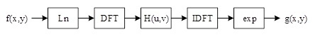
After filtering, the inverse Fourier transform is performed with \(s(x,y)=IDFT\left(S(u,v)\right)\). Finally, the output image is formed by taking the exponent of the filtered result as an inverse process: \[\label{GrindEQ__8_} g(x,y)=e^{s(x,y)} =i_{0} (x,y)r_{0} (x,y),\tag{8}\] where \(i_{0} (x,y)\) and \(r_{0} (x,y)\) are the irradiated and incident components of the processed image, respectively. The whole process of homomorphic filtering is shown in Figure 1.
In order to better control the irradiated and reflected components, the function \(H(u,v)\) of the above filter uses a deformation of the Gaussian high-pass filter to process the image, i.e., \[\label{GrindEQ__9_} H(u,v)=D^{2} \left(\gamma _{H} -\gamma _{L} \right)\left[1-e^{-c\left[D{'} (u,v)/D_{n} {'} \right]} \right]+\gamma _{L} .\tag{9}\]
In this case, choosing \(\gamma _{H} >1\) and \(\gamma _{L} <1\) achieves attenuating the contribution of low frequencies and enhancing the contribution of high frequencies, ultimately compressing the dynamic range of the image and enhancing the contrast of the image at the same time. The constant \(c\) controls the sharpness of the function slope, and \(D(u,v)\) and \(D_{0}\) denote the distance to the frequency center and the cutoff frequency, respectively. The larger \(D_{0}\) is, the more obvious the enhancement of image details.
In order to improve the efficiency of image algorithm analysis and development, this paper will use the German HALCON 8.0 software to analyze and process the image algorithm, the actual algorithm prototype, verify the algorithm through and then further transplant the algorithm to the host computer and DSP.
At present, more attention is paid to the hardware part of the system and image acquisition, and less attention is paid to the image processing and analysis part. An advanced machine vision system needs high-performance software in addition to high-performance hardware, and many common development software such as Microsoft’s VisualC++, NI’s LabWindows/CVI, etc. can be used for the development of machine vision system, but the development cycle is relatively long and the targeting of the machine vision system is not easy. Many common development software such as VisualC++ of Microsoft, LabWindows/CVI of NI can develop machine vision system, but the development cycle is longer, the target is weaker, and the complexity of program is higher. HALCON, the machine vision software from MVTec, is recognized as the machine vision software with the best performance. Using HALCON as the core software for machine vision and image processing can greatly shorten the development cycle and reduce the development difficulty.
Machine vision software HALCON is widely used in the world, users can take advantage of its open structure to quickly develop image processing and machine vision applications. A professional image processing tool contains more than just a library of image processing functions. The image processing task solves only a part of the overall machine vision solution, but also includes software parts such as processing controls and database connections, and hardware parts such as image acquisition and its illumination. Therefore, it is very important that the image processing system is easy to use and can be flexibly embedded into the development project.
Mathematical morphology uses structural elements with a certain shape as a tool to measure and extract the corresponding shape features in an image in order to analyze and identify the image. Mathematical morphology can be applied to maintain its basic shape features, simplify the image data, and remove extraneous structures.
The basic morphology is expansion and erosion, from these two transformations more morphological operations like open and closed operations can be defined.
The main types of mathematical morphology are binary morphology and grayscale morphology, in which the object of operations in binary morphology is the set, let \(X\) and \(B\) be the set of points in Euclidean space, generally \(X\) is the set of images (or dataset), and \(B\) is the structural element [1].
The expansion uses vector addition to merge two sets. The expansion is the set of the sum of all possible vectors added, the two operands of vector addition come from \(X\) and \(B\) and are taken to any possible combination. The definition of an expansion is shown below: \[\label{GrindEQ__10_} Dilation\left(X,B\right)=\left\{p\in \varepsilon ^{2} :p=x+b,x\in X\; And\; b\in B\right\}.\tag{10}\]
The effect of the expansion operation is to merge the background points around the target image into the object. If two objects are relatively close to each other, then the expansion operation will connect the two objects together. Expansion is useful to fill the voids in the objects after image segmentation.
Erosion uses vector subtraction for set elements, and Erosion is the dual operation of expansion. The definition of corrosion expansion Erosion is shown below. \[\label{GrindEQ__11_} Erosion\left(X,B\right)=\left\{p\in \varepsilon ^{2} :p+b=x,\mathrm{}or{\rm \; }every\; b\in B \right\}.\tag{11}\]
The role of erosion in mathematical morphology operations is to eliminate target image boundary points. Corrosion can remove objects that are smaller than the structural elements, and by selecting structural elements of different sizes, objects of different sizes can be removed. If there is a small connectivity between two objects, the corrosion operation can separate the two objects when the structural element is large enough.
Erosion and expansion are not inverse operations. If an image is first corroded and then expanded, the result is not the original image.
Open operation (Opening) is to use the same structural elements of the image first corrosion and then expansion of the operation. The definition of the Opening operation is shown below. \[\label{GrindEQ__12_} Opening\left(X,B\right)=Dilation\left(Erosion\left(X,B\right),X\right).\tag{12}\]
Open operation plays the role of polishing edges, that is, you can make the image of some of the sharp corners of the background into the background, the image processing with open operation, you can eliminate the details, so that the boundary is smooth, to eliminate the sharp peaks, flanges, cut off the narrow fine connection.
Closed operation is to use the same structural elements of the image first expansion and then corrosion operation. The definition of closed operation is shown below: \[\label{GrindEQ__13_} Clo\sin g\left(X,B\right)=Erosion\left(Dilation\left(X,B\right),X\right).\tag{13}\]
The closure operation fills in small holes and connects two neighboring targets, filters the outside of the image, and smoothes out sharp corners protruding into the inside of the image, making the edges of objects smoother.
Different pattern recognition theories and methods are used for different objects and purposes. Currently the main pattern recognition techniques include: statistical pattern recognition, syntactic structure pattern recognition, fuzzy pattern recognition, artificial neural network method and artificial intelligence method.
Pattern recognition is the process of processing and analyzing various forms of information (numerical, textual, and logical) that characterize a thing or phenomenon in order to describe, identify, classify, and explain it, and is an important part of information science and artificial intelligence.
Pattern recognition assumes that an image may contain one or more objects and that each object belongs to a number of predefined types, categories, or patterns. Given a digital image containing multiple objects, the pattern recognition process consists of three main stages, as shown in Figure 2.

Since the 80’s, with the neuroscientist’s in-depth study of the brain information processing, as well as the need for the development of computer science and artificial intelligence, the nonlinear large-scale parallel distributed processing as the mainstream of the neural network system has been developed rapidly, the use of neural network approach to the study of pattern recognition, as well as the use of neural computational structure to realize pattern recognition and artificial intelligence system has become a research hotspot.
Artificial neural network (ANN) is a complex network system consisting of a large number of simple processing units similar to neurons widely interconnected. It is proposed on the basis of the results of modern neural research and reflects several features of human brain function, but is not a real depiction of the nervous system, but only its simplification, abstraction and simulation. Through the adjustment of connection strengths, neural networks exhibit learning, generalization and classification characteristics similar to those of the human brain.
Learning algorithms for neurons can be divided into two categories: supervised and unsupervised. Supervised learning algorithms require that both the input and the correct output be given. The network adjusts the network based on the difference between the current output and the required target output so that the network reflects correctly. The best known algorithm of this type is the Backward Error Propagation (BP) algorithm for networks with implicit layers (). Unsupervised learning algorithms require only a set of inputs, and the network is able to gradually evolve to respond specifically to a certain pattern of inputs, typically such as competitive learning algorithms.
Among the various artificial neural network models, the most widely and successfully applied in pattern recognition is the multilayer feedforward network, which in turn is represented by the multilayer perceptron using the BP learning algorithm (conventionally abbreviated as BP network). Since the network is trained using supervised learning, it can only be used for supervised pattern recognition problems [16].
In this paper, the number of implicit layer nodes is calculated using the following empirical formula: \[\label{GrindEQ__14_} m=\left\{\begin{array}{ll} {n+0.618\left(n-t\right)} & {n\ge t}, \\ {t-0.618\left(t-n\right)} & {n<t}, \end{array}\right.\tag{14}\] where \(n\), \(m\), \(t\) are the number of nodes in the input, hidden and output layers, respectively.
For the food foreign object category classifier, substituting \(n=3\), \(t=6\) into Eq. (14) yields the number of nodes in the hidden layer \(m=4\).
In the training phase of the network, if the category label of the input training sample is \(i\), the expected output of the \(i\)th node is 1, and the rest of the output nodes are 0. In the recognition phase, when a sample of an unknown category is acted on the input, the outputs of the nodes are examined and the category of this sample is determined to be the one that corresponds to the largest output node. In some cases, if the difference between the node with the largest output and the outputs of the other nodes is small (less than a certain threshold), a rejection decision can be made. This is the most basic approach to pattern recognition with multilayer perceptrons.
The BP algorithm belongs to the \(\delta\) algorithm, which is a learning algorithm with a tutor, and the basic idea of its structure is: for \(P\) input learning samples: \(x_{1} ,x_{2} ,\cdots ,x_{p}\), the output samples corresponding to them are known to be: \(t_{1} ,t_{2} ,\cdots ,t_{p}\), and the errors of the actual outputs \(y_{1} ,y_{2} ,\cdots ,y_{p}\) and \(t_{1} ,t_{2} ,\cdots ,t_{p}\) are used to modify the connection weights and the thresholds, so as to make the \(y_{i} \left(i=1,2,\cdots p\right)\) and the desired \(t_{i}\) as close as possible to each other, so that the sum of squares of the errors in the output layer of the network is minimized.
The network structure is set to contain only \(n\) hidden layer, with one input neuron, \(s\) hidden layer neurons and activation function \(f_{j}\), \(m\) neurons in the output layer with corresponding activation function \(f_{k}\), an output of \(Y\), and a target vector of \(T\). The output of the \(j\)th neuron in the hidden layer is: \[\label{GrindEQ__15_} y_{j} =f_{j} \left(\sum\limits_{i=1}^{n}w_{ji} x_{i} +b_{j} \right)\left(j=1,2,\cdots ,s\right),\tag{15}\] where \(y_{j}\) is the output of node \(j\), \(w_{ji}\) is the connection weights between nodes, and \(b_{j}\) denotes the threshold value.
And the output of the \(k\)th neuron of the output layer is: \[\label{GrindEQ__16_} y_{k} =f_{k} \left(\sum\limits_{j=1}^{k}w_{kj} y_{j} +b_{k} \right)\left(k=1,2,\cdots m\right).\tag{16}\]
Define the error function as: \[\label{GrindEQ__17_} E\left(W,B\right)=1/2\sum\limits_{k=1}^{m}\left(t_{k} -y_{k} \right)^{2} .\tag{17}\]
Then the weights of the output layer change as: \[\label{GrindEQ__18_} \Delta w_{kj} =-\eta \frac{\partial E}{\partial w_{kj} } =-\eta \frac{\partial E}{\partial y_{k} } \frac{\partial y_{k} }{\partial w_{kj} } =\eta \left(t_{k} -y_{k} \right)f_{k} y_{j} =\eta \delta _{kj} y_{j} ,\tag{18}\] where \(\eta\) is the learning rate, and it has been shown that \(\eta\) is usually taken to be close to 1. Then \[\label{GrindEQ__19_} \delta _{kj} =\left(t_{k} -y_{k} \right)f_{k} =e_{k} f_{k} e_{k} =t_{k} -y_{k} .\tag{19}\]
Similarly, \[\label{GrindEQ__20_} \Delta b_{k} =-\eta \frac{\partial E}{\partial b_{k} } =-\eta \frac{\partial E}{\partial y_{k} } \frac{\partial y_{k} }{\partial b_{k} } =\eta \left(t_{k} -y_{k} \right)f_{k} =\eta \delta _{kj} .\tag{20}\]
For the change of weights in the implicit layer, i.e., from the \(i\)th input to the \(j\)th output the weights are: \[\label{GrindEQ__21_} \begin{array}{rcl} {\Delta w{}_{ji} } {=} {-\eta \frac{\partial E}{\partial w_{ji} } =-\eta \frac{\partial E}{\partial y_{k} } \frac{\partial y_{k} }{\partial y_{j} } \frac{\partial y_{j} }{\partial w_{ji} } } {=} {\eta \sum \left(t_{k} -y_{k} \right) f_{k} w_{kj} f_{j} x_{i} =\eta \delta _{ji} x_{i} }, \end{array}\tag{21}\] where \(\delta _{ji} =e_{j} \cdot f_{j}\), \(e_{j} =\sum\limits_{k=1}^{m}\delta _{kj} w_{kj}\).
Similarly, \[\label{GrindEQ__22_} \Delta b_{j} =\eta \delta _{ji} .\tag{22}\]
Although the backpropagation method has a solid theoretical basis, a rigorous derivation process, beautiful symmetry of the resulting formulas, clear physical concepts (error backpropagation), and a high degree of generality. Due to these advantages, it is still the predominant learning algorithm for multilayer forward neural networks. Despite the above contributions and advantages of the BP algorithm, it has been found that BP itself has many shortcomings in use, i.e., there are some problems that need to be improved.
Over the past decade, many researchers have made in-depth studies on the problem and proposed many improvement methods. Among them, the most commonly used ones are additional momentum method and adaptive learning rate method.
Additional momentum method.
The additional momentum method modifies the weights not only according to the current negative gradient direction of the objective function, but also takes into account the influence of the change trend on the error surface, i.e., the previous negative gradient direction, so that the training may jump out of the local minima. The way it modifies the weights is: \[ \Delta W_{ji} \left(k+1\right)=\left(1-mc\right)\eta \delta _{i} p_{j} +mc\Delta W_{ji} \left(k\right), \tag{23}\]\[ \Delta b_{i} \left(k+1\right)=\left(1-mc\right)\eta \delta _{i} +mc\Delta b_{i} \left(k\right), \tag{24}\] where, \(k\) is the number of training times and \(mc\) is the momentum factor, which is generally taken around 0.95.
Adaptive learning rate method.
This method automatically adjusts the learning rate according to the convergence of the network during the training process, i.e., when the new error exceeds a certain multiple of the old error, the learning rate decreases; when the new error is smaller than the old error, the learning rate increases; otherwise, it remains unchanged.
Other methods.
Change the return error to: \[\label{GrindEQ__24_} \varepsilon _{i} =\left(f'+pc\right)e_{i} ,\tag{25}\] where \(pc\) is a correction factor that can be adaptively adjusted according to the network convergence.
When the type \(S\) action function is used, the larger weighted sum will enter the saturation region of the type \(S\) function, which makes the value of \(f'\) very small, and thus the return error \(\varepsilon _{i}\) is also very small, which ultimately results in almost stagnation of the weight modification. The introduction of correction coefficients improves this phenomenon and avoids the phenomenon of network hemp seeding.
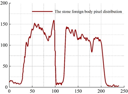
The distribution characteristics of line gray scale in the ray image is an important basis for the determination of foreign objects in the image, thus the line gray scale curves of various typical foreign objects in the image are analyzed, and the line curve gray scale characteristics are very important for the ability to accurately determine the foreign objects. Line pixel values are extracted using the denoised and enhanced dataset of food ray images containing three different foreign objects. The three images containing different foreign objects are compared with the line pixel distribution curves at the point where the foreign object is located and at the point where the foreign object is not contained.
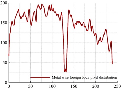
As shown in the figure, it can be clearly seen from the comparison graph. The gray level curve of the rows where the foreign objects are located, there are abnormal points, which are very different from the pixels that do not contain the foreign objects, and are shown as a large distribution of ups and downs on the gray level curve of the rows. For metal, stone, glass, such as the density difference with the examined food is relatively large foreign matter, due to its strong absorption ability of the ray of this kind of foreign matter where the line pixel value distribution curve will usually appear large fluctuations, after calculating three kinds of foreign matter where the line were 132, 108, 34, and does not contain foreign matter of the food in the same position at the grayscale value of the difference between the big, so that we can identify the existence of foreign matter.
Figure 3 shows the distribution curve of pixel values in the rows without foreign matter, and Figure 4 shows the distribution curve of pixel values in the rows of metal wire foreign matter. There is a significant fluctuation around 128 to 136.
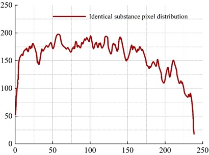
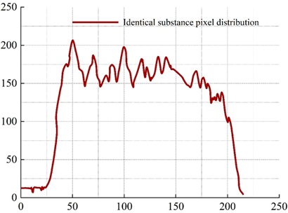
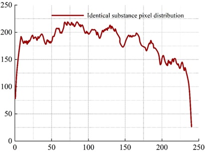
Figure 5 shows the distribution curve of pixel values in the no foreign body row and Figure 6 shows the distribution curve of pixel values in the stone foreign body row. A significant fluctuation around 101 to 119 can be clearly seen in Figure 6.
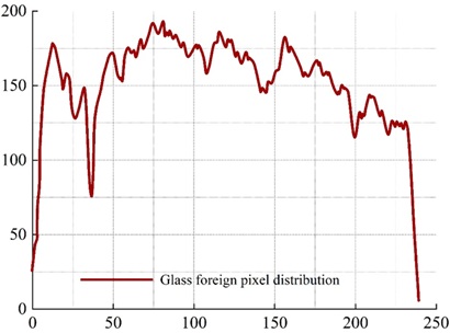
Figure 7 shows the distribution curve of pixel values in the no foreign body row and Figure 8 shows the distribution curve of pixel values in the glass foreign body row. A significant fluctuation around 31 to 37 can be clearly seen in Figure 8.
After obtaining the gray curve distribution of the image, it is further analyzed. Table 1 shows some of the sample data used in the training of the network, through which the network is trained and the network weights are constantly adjusted so that the output vector of the network is constantly close to the classification target and the individual weights of the network connection are obtained.[]
| Eigenvalue | K | e | \(\delta\) | Expected output | Foreign matter | ||
|---|---|---|---|---|---|---|---|
| 1 | 0.23 | 0.89 | 0.6 | 0 | 0 | 1 | Wire |
| 2 | 0.39 | 0.82 | 0.62 | 0 | 0 | 1 | |
| 3 | 0.23 | 0.68 | 0.54 | 0 | 0 | 1 | |
| 4 | 0.26 | 0.84 | 0.58 | 0 | 0 | 1 | |
| 5 | 0.17 | 0.92 | 0.56 | 0 | 0 | 1 | |
| 6 | 1.03 | 0.11 | 0.31 | 0 | 1 | 0 | Stone |
| 7 | 0.75 | 0.24 | 0.36 | 0 | 1 | 0 | |
| 8 | 0.93 | 0.19 | 0.24 | 0 | 1 | 0 | |
| 9 | 0.99 | 0.15 | 0.22 | 0 | 1 | 0 | |
| 10 | 0.85 | 0.27 | 0.31 | 0 | 1 | 0 | |
| 11 | 0.31 | 0.72 | 0.78 | 1 | 0 | 0 | Glass |
| 12 | 0.27 | 0.41 | 0.8 | 1 | 0 | 0 | |
| 13 | 0.45 | 0.57 | 0.86 | 1 | 0 | 0 | |
| 14 | 0.32 | 0.62 | 0.84 | 1 | 0 | 0 | |
| 15 | 0.39 | 0.81 | 0.82 | 1 | 0 | 0 | |
The training samples stone, wire, and glass were each taken as three eigenvalue samples as a test set, and the test results are shown in Table 2.
By using the data in the limited test sample set to predict the network, the results show that the defect classification correct rate of the network basically meets the experimental requirements. Judgment is made on the output results of the test data, for the number of output result values greater than 0.5, it is judged as 1; for the number less than 0.5, we judge it as 0, and finally the detection results are obtained. From the recognition rate after detection, the three kinds of foreign objects have reached 100%, but in fact from the output results of the data carefully analyzed, the detection of metal wires in the second line of data reached 0.4147442681640707, the detection of stones in the third line of 0.4775917723570386, the value of these data has been close to 0.5, indicating that can be judged to be the accuracy of the 0 rate in the reduction of. The possibility of misjudgment of the presence of foreign objects exists, and the judgment of the type of defect will be inaccurate.
The reason for the misjudgment of foreign objects is mainly due to the change of foreign object characteristic value:
Stone misclassification.
some stones are nearly triangular in shape, while the glass shape may also appear quadrilateral and multi-deformation, the stone and glass have the same possibility in the value of circularity e. The main difference between stone and glass is the gray deviation of the foreign matter itself \(\delta\). When the ratio of the longitudinal and transverse axes of the nearly triangular stone is larger than K, and the degree of circularity e is not high, if the density of the stone is not too homogeneous, the change of the gray deviation of the foreign matter itself \(\delta\) increases, although the value of \(\delta\) is still smaller than the value of glass, but the stone can be misclassified as glass easily. , although the value of \(\delta\) of the stone is still smaller than that of the glass, the stone is easy to be misjudged as glass.
Metal wire misjudgment.
the biggest difference between metal wire and stone and glass is that the ratio of longitudinal and transverse axes K is the largest, but the roundness e of metal wire and finer stone is closer, so part of metal wire may be misjudged as glass.
Misjudgment of glass.
The difference in gray scale deviation \(\delta\) between glass, metal wire, stones and other foreign materials is very large, and the difference in the value of roundness e between glass and metal wire is also very large, so the possibility of misjudgment as stones and metal wire is the smallest.
| Defect type | K | e | \(\delta\) | Output result | Test result | Recognition rate |
|---|---|---|---|---|---|---|
| Wire | 0.23 | 0.86 | 0.68 | 0.022569085848090; | 0,0,1 | 100% |
| 0.0001859073855550; | ||||||
| 0.9972037119614731 | ||||||
| 0.23 | 0.82 | 0.72 | 0.4147442681640707; | 0,0,1 | ||
| 0.0007106236676049; | ||||||
| 0.7778365923359559 | ||||||
| 0.23 | 0.69 | 0.62 | 0.2611933204290650; | 0,0,1 | ||
| 0.0007231335880791; | ||||||
| 0.9009081055541353 | ||||||
| Stone | 0.98 | 0.22 | 0.31 | 0.0001987673762857; | 0,1,0 | 100% |
| 0.9996305342787899; | ||||||
| 0.0008735563648794 | ||||||
| 0.83 | 0.32 | 0.41 | 0.0074822934898709; | 0,1,0 | ||
| 0.9917714563437915; | ||||||
| 0.0004982780794820 | ||||||
| 0.99 | 0.34 | 0.22 | 0.0000008257278707; | 0,1,0 | ||
| 0.9995832616775387; | ||||||
| 0.4775917723570386 | ||||||
| Glass | 0.2 | 0.57 | 0.77 | 0.9993642320030504; | 1,0,0 | 100% |
| 0.00058361416377080; | ||||||
| 0.0002405881301942 | ||||||
| 0.4 | 0.63 | 0.84 | 0.9998658506143140; | 1,0,0 | ||
| 0.0016301418372215; | ||||||
| 0.0000407935772125 | ||||||
| 0.31 | 0.25 | 0.81 | 0.9999755735428054; | 1,0,0 | ||
| 0.0027902532728969; | ||||||
| 0.0000020270483593 |
In this paper, a pattern recognition method based on image recognition for food foreign objects is proposed to achieve food safety detection. Experiments are carried out on the dataset of food ray images containing three different foreign objects after denoising and enhancement, and the row pixel distribution curves are compared, and the rows of the three kinds of foreign objects are calculated to be 132, 108 and 34 respectively, which are larger than the grayscale values of food products without foreign objects at the same position, thus the existence of foreign objects can be identified, and the performance of the algorithm designed in this paper is preliminarily verified. In the analysis of the actual application effect, the recognition rate of the three kinds of foreign objects reached 100%, and analyzed the main reasons why the foreign objects were misjudged.