
Ribonucleic acid (RNA) plays an important role in various biological processes within cells, ranging from catalytic activity to gene expression. An RNA molecule is described by its sequence of bases: A (adenine), U (uracil), G (guanine), and C (cytosine). RNA sequences have a chemical orientation from their sugar-phosphate backbones. This orientation is designated by end labels \(5^{\prime}\) and \(3^{\prime}\), with the \(5^{\prime}\) end typically appearing on the left. Helical structures are formed using the base sequences where A pairs with U while G pairs with C (and sometimes the non-Watson-Crick base pair G with U), and these helical structures consistent with certain planar graphs are known as RNA secondary structures.
More than four decades ago, Waterman and his coworkers pioneered the combinatorial and computational study of RNA secondary structures [19, 20, 23, 24]. Since then, there have been lots of works in the field, see [6, 8, 9, 10, 12, 13, 14, 15, 16, 17] and references therein. For example, enumeration of RNA secondary structures by some structural characteristics, like hairpins and cloverleaves [23], and base pairs [18] was first studied. Subsequently, further filtrations of RNA secondary structures were analyzed, as for instance, stacks, components, loops by Hofacker, Schuster and Stadler [12], orders of structures by Nebel [17], hairpins and cloverleaves by Liao and Wang [14], Chang and Zeng [1], and Helm et al. [11], saturated structures by Clote [6], the \(5^{\prime}\)–\(3^{\prime}\) end distance by Clote, Ponty and Steyaert [7], Han and Reidys [9], and the rainbow spectrum by Li and Reidys [13].
It is fair to say that the recursive nature of RNA secondary structures is well understood. Thus, it is possible to use recursion to count secondary structures by certain structural characteristics, and then obtain functional relations of the corresponding generating functions. However, it is not necessarily easy to derive exact formulae as in Schmitt and Waterman [18] and the majority of the contributions in the field is concerned with asymptotic results. In [18], the exact number of secondary structures over a sequence of length \(n\) that have \(k\) base pairs is obtained by establishing a bijection between secondary structures and plane trees, and then enumerating the corresponding plane trees, e.g. by Chen’s bijective approach [5].
Recently, the author discovered a new bijection \(\varphi\) between RNA secondary structures and plane trees [2], which gives rise to a new bijection on plane trees when combined with the Schmitt-Waterman bijection [18]. Based on the bijection \(\varphi\), exact and explicit formulae counting RNA secondary structures according to the number of stacks and the joint length distribution of stacks and loops were obtained for the first time in Chen, Reidys and Waterman [4], while some related asymptotic results, e.g. Hofacker, Schuster and Stadler [12], have been known for about two decades.
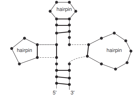
Among different kinds of loops, hairpin loops (or hairpins) are among the most important and have been extensively studied [1, 11, 14, 21, 22, 23]. In particular, certain subsets of secondary structures characterized by the number of contained hairpins and the way how these hairpin loops are organized have been enumerated in a variety of works, mostly asymptotically. For instance, general hairpins and general cloverleaves have been studied in [1, 14, 23]. An example of a general cloverleaf is illustrated in Figure 1, where a general cloverleaf is an arrangement of hairpin loops in a circular manner, and a general hairpin is basically the same as a general cloverleaf with the exception that there are no base pairs at the \(5^{\prime}\)-end and \(3^{\prime}\)-end (i.e. base pairs in the bottom part of Figure 1).
The main objective of the present work is to generalize the enumeration of general hairpins as well as cloverleaves and to exactly enumerate general RNA secondary structures with a given number of stacks and hairpin loops, regardless of their organization. Our approach is based on the bijection \(\varphi\) and purely combinatorial.
In this section, we review the bijection \(\varphi\) [2]. We first recall the definition of RNA secondary structures following Waterman [24]. Let \([n] = \{ 1,2, \ldots, n\}\). An RNA secondary structure of length \(n\) is a simple graph with vertices in \([n]\), every vertex having degree at most one, and edges in \(E\) satisfying
if \((i,j)\in E\), then \(|i-j|\geq 2\);
if \((i,j)\in E\) and \((k,l)\in E\), where \(i < j\) and \(k < l\), and \([i,j] \bigcap [k, l]\neq \varnothing\), then either \([i,j]\subset [k, l]\) or \([k, l] \subset [i,j]\) (where \([i,j]\) denotes the interval \(\{r: i\leq r \leq j\}\)).
We typically draw an RNA secondary structure as follows: we place all vertices in a horizontal line and we draw an edge as an arc in the upper half-plane. Then, the second condition in the above definition guarantees that any two arcs do not cross with each other. An arc determines a base pair. The vertex of an arc with a smaller label is called the left-end of the arc, and a vertex not adjacent to any edge is called an isolated base. In addition, if \((i,j)\) is an arc, we say that another arc \((i_1,j_1)\) (resp. an isolated base \(k\)) is covered by \((i,j)\) if \([i_1,j_1]\subset [i,j]\) (resp. \(k\in [i,j]\)), and we also say that the arcs \((i,j)\) and \((i_1, j_1)\) nest with each other. Sometimes another way of graphing an RNA secondary structure like Figure 1 is applied.
A plane tree \(T\) is an unlabeled, rooted tree, where its subtrees are also plane trees and linearly ordered. In a plane tree \(T\), the number of edges in the unique path from a vertex \(v\) to the root of \(T\) is called the level of \(v\), and the vertices adjacent to \(v\) on a higher level are called the children of \(v\). The vertices on level \(2i\) (resp. \(2i-1\)) for \(i\geq 0\) are called even-level (resp. odd-level) vertices. A vertex without any child is called a leaf, and an internal vertex otherwise. The root of a plane tree is always treated as internal. The outdegree of a vertex is the number of children of the vertex. We will draw plane trees with the root on the top level, i.e., level \(0\), and with the children of a level \(i\) vertex arranged on level \(i+1\) left-to-right following their linear order.
Chen’s bijection \(\varphi\) [2]. Let \(R\) be an RNA secondary structure of length \(2a+k\) with \(k\) isolated bases. We construct a plane tree \(\varphi(R)\) as follows:
S1: Add an auxiliary arc \((0, 2a+k+1)\). Label the isolated bases in \(R\) with \(b_1,b_2,\ldots, b_k\) left-to-right, and label the arcs with \(e_0, e_1,\ldots, e_a\) based on the left-to-right order of their left-ends, \(e_0\) being \((0, 2a+k+1)\).
S2: Let \(b_1\) be the root of \(\varphi(R)\), and generate \(k_1\) children for \(b_1\) if there are \(k_1\) arcs covering the isolated base \(b_1\), where the children from left to right correspond to these \(k_1\) arcs from the outermost to the innermost and are labeled accordingly.
S3: For \(j=2\) to \(k\), put a new child to the left of all existing children of the vertex that corresponds to the innermost arc covering the isolated base \(b_j\) in the current partially constructed tree and label the newly generated child with \(b_j\). Next generate \(k_j\) children for the vertex \(b_j\) if there are \(k_j\) unused arcs (i.e., those with labels not appearing in the current partial tree) covering the isolated base \(b_j\), where again the children from left to right correspond to these \(k_j\) arcs from the outermost to the innermost and are labeled accordingly.
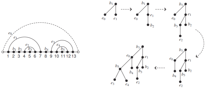
Then it is not difficult to see: (i) the vertices \(b_i\) correspond to the even-level vertices in \(\varphi(R)\), (ii) the sequence \(e_0e_1\cdots e_a\) will be obtained if the children of even-level vertices (in the order \(b_1b_2\cdots b_k\)) are collected left-to-right sequentially; (iii) the sequence \(b_1b_2\cdots b_k\) will be obtained if the even-level vertices are searched by depth-first search from right to left. So, the labels of the vertices can be easily and uniquely recovered after being removed. Therefore, the obtained structure is essentially a plane tree with \(a+k\) edges.
See Figure 2 for an example. We refer to [2] for details about the bijection.
Let \(R\) be an RNA secondary structure of length \(n\). We call the RNA secondary structure \(\hat{R}\) obtained from \(R\) by adding the auxiliary arc \((0, n+1)\) the canonical form of \(R\), or a canonical RNA secondary structure (of length \(n\)). Thus, every canonical RNA secondary structure has at least one arc. Conversely, given a canonical RNA secondary structure \(\hat{R}\), it is clear what the underlying RNA secondary structure \(R\) is.
Definition 3.1(Partial stack). A partial stack in an RNA secondary structure (irrespective of canonical or not) is a sequence of consecutive bases \(x, x+1, \ldots, x+k-1\) for some \(x\geq 0,\; k>0\) that are left-ends of some arcs while \(x-1\) and \(x+k\) are isolated bases (or \(x-1\) is not a base and/or \(x+k\) is not a base).
Equivalently, a partial stack is a maximal set of mutually nesting arcs whose left-ends are consecutive. The number \(k\) is called the length of the partial stack. Partial stacks are first introduced in [4].
Definition 3.2(Stack). A stack in an RNA secondary structure is a set of arcs mutually nesting with each other such that both the left-ends and right-ends are respectively consecutive, and no other such a set constains the present set of arcs as a subset (i.e., maximal).
A stack is called a helix sometimes. Loops in RNA secondary structures have been extensively studied, as they are important for certain energy models predicting the folded secondary structure of a given RNA (primary) base sequence. A loop consists of a set of isolated bases that are directly covered by the same arc [12], i.e. the innermost arc covering these isolated bases. The length of the loop is the size of the set, and we refer to the arc as the arc of the loop. The degree of a loop is one larger than the number of arcs directly covered by the arc of the loop [12].
Loops have been classified into different types: hairpin loops, interior loops, bulges, and multi-loops.
Definition 3.3(Hairpin). A hairpin loop is a loop where the arc of the loop does not cover any arcs, i.e. degree one.
For example, in Figure 2 (left), \(\{5\}, \{11\}\) are hairpin loops. An interior loop is a loop where there exists exactly one arc directly covered by the arc of the loop and separating at least two isolated bases (i.e., one is to the left and one is to the right).
Definition 3.4 (Bulge). A bulge is an interior loop such that either the left-ends or the right-ends of the arc of the interior loop and the arc directly covered by it are consecutive.
We call bulges of the first case right-bulges (or \(3^{\prime}\)-bulges) and that of the second case left-bulges (or \(5^{\prime}\)-bulges). For example, in Figure 2 (left), \(\{2,3\}\) gives a left-bulge. Other loops, i.e. degree larger than two, are called multi-loops.
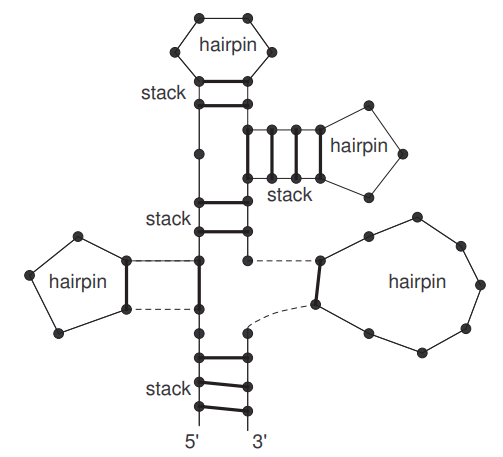
An example of an RNA secondary structure with hairpins and stacks displayed is shown in Figure 3. In the following, we shall combinatorially enumerate RNA secondary structures according to stacks and hairpin loops.
First, we collect some known results from the previous work [4].
Lemma 3.5([4]). The number of canonical RNA secondary structures with \(b+1\) (\(b\geq 0\)) base pairs, \(k\) isolated bases and \(l\) partial stacks is the same as the number of plane trees with \(b+k\) edges and \(k\) even-level vertices \(l\) of which are internal.
Lemma 3.6([4]). Let \(\hat{R}\) be a canonical RNA secondary structure. The length of a partial stack of \(\hat{R}\) uniquely corresponds to the outdegree of an even-level vertex in \(\varphi(R)\).
Lemma 3.7 ([4]). Let \(\hat{R}\) be a canonical RNA secondary structure. The size of a loop of \(\hat{R}\) uniquely corresponds to one plus the outdegree of an odd-level vertex in \(\varphi(R)\).
In a plane tree, we call a maximal set of (left-to-right) consecutive odd-level leaves and an immediately following odd-level internal vertex if any that are children of the same even-level vertex a E-block. By definition, for an even-level internal vertex \(v\), if its rightmost child is an internal vertex, then the number of E-blocks of \(v\) (i.e. determined by \(v\)) is the number of odd-level internal vertices that are children of \(v\); otherwise, the number of E-blocks determined by \(v\) is one plus the number of odd-level internal vertices that are children of \(v\).
Proposition 3.8([4]). Let \(\hat{R}\) be a canonical RNA secondary structure. Then, the number of stacks in \(\hat{R}\) equals the number of E-blocks in \(\varphi(R)\). In addition, the size of a stack of \(\hat{R}\) uniquely corresponds to the size of a E-block in \(\varphi(R)\).
Lemma 3.9. Let \(\hat{R}\) be a canonical RNA secondary structure. Then, the number of hairpin loops in \(\hat{R}\) equals the number of odd-level vertices that are respectively the rightmost children of some even-level vertices and respectively have leaves as the only children (if any) in \(\varphi(R)\). In addition, the length of a hairpin loop of \(\hat{R}\) uniquely corresponds to one larger than the number of children of such an odd-level vertex in \(\varphi(R)\).
Proof. The arc of a hairpin loop in \(\hat{R}\) is obviously the innermost arc among the arcs associated to a partial stack. Thus, from Chen’s bijection, the arc of a hairpin loop corresponds to the rightmost child of an even-level vertex in \(\varphi(R)\). The children of the arc (as a vertex) of a hairpin loop are obviously the isolated bases except the leftmost one covered by the arc. Since there are no other arcs covering these isolated bases, these isolated bases appear as leaves in \(\varphi(R)\), completing the proof. ◻
As an example illustrating Lemma 3.9, we can inspect the two hairpin loops in the RNA secondary structure in Figure 2 whose arcs are respectively \(e_2\) and \(e_4\).
Lemma 3.10. Let \(\hat{R}\) be a canonical RNA secondary structure. Then, the number of right-bulges in \(\hat{R}\) is the number of odd-level internal vertices that are not the rightmost children of any even-level vertices and respectively have leaves as the only children in \(\varphi(R)\).
Proof. By definition, the arc \(e\) of a right-bulge is not the innermost arc of a partial stack, thus the corresponding vertex in \(\varphi(R)\) is not the rightmost child of any even-level vertex. By definition, all but the leftmost element directly covered by \(e\) are isolated bases, and according to \(\varphi\), those isolated bases constitute the children of \(e\), all being leaves, and the lemma follows. ◻
For some practical reasons, there may be some requirements on the minimum length \(\theta\) (typically \(\theta \geq 2\)) of a stack and the minimum distance \(\sigma\) (typically \(\sigma \geq 3\)) of the two bases of a base pair, i.e., \(|j-i|>\sigma\) if bases \(i\) and \(j\) form a base pair. Note that the latter is equivalent to requiring the minimum length of a hairpin loop being \(\sigma\) as every base pair is either an arc of a hairpin loop or covering a hairpin loop. In the following, our enumeration will be based on \(\sigma>1\). The case of \(\sigma=1\) is slightly different, but it can be dealt analogously.
Lemma 3.11. For a canonical RNA secondary structure \(\hat{R}\) with \(\sigma>1\), the number of E-blocks in \(\varphi(R)\) is the same as the number of odd-level internal vertices, or equivalently, the rightmost child of any even-level internal vertex is internal.
Proof. There are the following two cases. For a given even-level internal vertex, if the rightmost child \(e\) corresponds to an arc which is not the arc of a hairpin loop, then the arc covers at least another arc. From Chen’s bijection, the leftmost isolated base covered by the latter must be a child of \(e\). Thus, \(e\) is an odd-level internal vertex; If \(e\) corresponds to an arc which is an arc of a hairpin loop, since there are \(\sigma>1\) isolated bases covered by \(e\), \(e\) must have \(\sigma-1>0\) children, as each isolated base other than the leftmost one induces a child of \(e\) according to Chen’s bijection. Thus, \(e\) is also an odd-level internal vertex, completing the proof. ◻
Based on Lemma 3.9 and Lemma 3.11, we obtain
Lemma 3.12. Let \(\hat{R}\) be a canonical RNA secondary structure with \(\sigma>1\). Then the number of hairpin loops in \(\hat{R}\) is the number of odd-level internal vertices that are respectively the rightmost children of some even-level vertices and have at least \(\sigma-1\) leaves as the only children in \(\varphi(R)\).
Now we are in a position to present a basic correspondence between RNA secondary structures and plane trees as follows.
Theorem 3.13. An RNA secondary structure \(R\) with \(b\) base pairs, \(k\) isolated bases, \(l_e\) partial stacks, \(s\) stacks of length at least \(\theta\), \(g\) right-bulges and \(h>0\) hairpin loops of length at least \(\sigma>1\) uniquely corresponds to a plane tree \(\varphi(R)\) in which there are \(k\) even-level vertices, \(b+1\) odd-level vertices, exactly \(h\) odd-level vertices that are respectively the rightmost children of some even-level vertices and have at least \(\sigma-1\) children all being leaves, and either
1. there are \(s+1\) E-blocks such that the leftmost E-block of the root is of size one while each of the rest of E-blocks is of size at least \(\theta\) and there are at least two E-blocks incident to the root, \(l_e\) even-level internal vertices, \(s+1\)
odd-level internal vertices where \(g+1\) of them are not the rightmost children of any even-level vertices and have leaves as the only children, or
2. there are \(s+1\) E-blocks such that there is exactly one E-block of size one incident to the root and each of the rest of E-blocks is of size at least \(\theta\), \(l_e+1\) even-level internal vertices, \(s+1\) odd-level internal vertices where \(g\) of them are not the rightmost children of any even-level vertices and have leaves as the only children, or
3. there are \(s\) E-blocks such that the leftmost E-block of the root is of size at least \(\theta+1\) while each of the rest of E-blocks has a size at least \(\theta\), \(l_e\) even-level internal vertices, \(s\) odd-level internal vertices where \(g\) of them are not the rightmost children of any even-level vertices and have leaves as the only children.
Proof. Let \(n=2b+k\). We just remark that the three cases come from the following three cases regarding the given RNA secondary structure \(R\): (1) \((1,n)\) is not a base pair but the base \(1\) is paired, (2) \((1,n)\) is not a base pair and \(1\) is an isolated base, (c) \((1,n)\) is a base pair. The rest should be clear from the above lemmas. ◻
Remark 3.14. An RNA secondary structure \(R\) with at least one base pair contains at least one hairpin loop, which implies the RNA secondary structure containing at least \(\sigma+2\) bases. In this case, it is clear that \(\hat{R}\) also satisfies the requirement of every hairpin loop being of length at least \(\sigma\).
Conversely, if there are no hairpin loops, then there are no base pairs. An RNA secondary structure \(R\) of length \(n<\sigma\) without base pairs satisfies the requirement of every hairpin loop having a length at least \(\sigma\) too, but \(\hat{R}\) does not. This is the reason that we require \(h>0\) in Theorem 3.13 for the sake of simplicity.
According to Theorem 3.13, enumerating RNA secondary structures by stacks and hairpin loops can be done by enumerating the corresponding plane trees. The latter can be achieved by enumerating certain labelled set-alternating trees. A labelled set-alternating E-tree (resp. O-tree) is a plane tree where the even-level vertices carry distinguishable labels from a set \(E\) (resp. \(O\)) and the odd-level vertices carry distinguishable labels from a set \(O\) (resp. \(E\)). We shall enumerate labelled set-alternating E-trees based on our variation of Chen’s bijection [5] dealing with uniformly (i.e. using only one set of labels) labelled plane trees.
In order to state our bijection motivated by Chen’s bijection [5], we set some notation. A forest is a set of trees. A (labelled) small tree is a (labelled) tree with only two levels in total. A small set-alternating tree is a set-alternating tree with only two levels. The size of a small tree is the number of edges in the small tree. We shall call a small set-alternating tree with a root in \(E\) (resp. \(O\)) a small E-tree (resp. O-tree).
Our bijection is between certain labelled set-alternating trees and certain forests consisting of some small E-trees and some small O-trees, where additional labels besides the ones used in the plane trees will appear in the forests. We shall mark each of the additional labels by \(^*\) and refer to them as starred labels. As the local structure of the children (e.g. distribution of leaves and internal vertices) of an odd-level internal vertex is not relevant, we call all children of an odd-level internal vertex an O-block. In the following, we sometimes refer to a vertex by its label.
Theorem 3.15. Suppose \(E=[k]\subset E^*=[k]\bigcup \{(k+1)^*, \ldots, (k+l_e-1)^*\}\) and \(O=[\overline{b+1} ] \subset O^*=[\overline{b+1}] \bigcup \{(\overline{b+2})^*, \ldots, (\overline{b+1+s})^*\}\). Then there is a bijection between the set \(\mathbb{T}\) of set-alternating trees over \(E\bigcup O\) with \(b+k\) edges and a root \(k\in E\), in which,
(a) there are exactly \(s\) E-blocks such that the leftmost E-block of the root has a size \(l\) (resp. at least \(l\)) and each of the rest has a size at least \(\theta\), and
(b) \(l_e\) even-level internal vertices, \(s\) odd-level internal vertices, and
(c) the vertices in \([\overline{h}]\) are the only odd-level internal vertices that are respectively the rightmost children of some even-level vertices and respectively have at least \(\sigma-1\) children all being leaves, and
(d) the vertices in the set \(\{\overline{h+1}, \ldots, \overline{h+g}\}\) are the only odd-level internal vertices that are not the rightmost children of any even-level vertices and have leaves as the only children,
and the set \(\mathbb{F}\) of forests of small set-alternating trees over \(E^* \bigcup O^*\) where in each forest:
(1) there are \(l_e\) small E-trees with roots from \(E\) such that the rightmost child of any small E-tree has a starred O-label, there is a small E-tree rooted on \(k\in E\) where the leftmost E-block has a size exactly \(l\) (resp. at least \(l\)) while the rest of E-blocks over these small E-trees have size at least \(\theta\) (a E-block in a small E-tree is a maximal set of consecutive vertices with unstarred labels and the following vertex with a starred label if any);
(2) there are \(h\) out of \(l_e\) small E-trees whose rightmost child has a label \((\overline{b+1+i})^*\) for some \(1\leq i \leq h\);
(3) the starred O-label \((\overline{b+1+s})^*\) must appear in the small E-tree rooted on \(k\);
(4) there are \(s\) small O-trees with roots from \(O\), among which \(h\) small O-trees of size at least \(\sigma-1\) have roots from the set \([\overline{h}]\) and do not have any starred labels, \(g\) small O-trees have roots from the set \(\{\overline{h+1}, \ldots, \overline{h+g}\}\) and do not have any starred labels, and any of the rest of \(s-h-g\) small O-trees has at least one starred label;
(5) the labels in the set \(\{ (\overline{b+2+h})^*, \ldots, (\overline{b+1+g+h})^*\}\) do not appear at the rightmost children of any small E-trees.
A proof of Theorem 3.15 will be given in the appendix. In the following, we shall enumerate the three classes of plane trees distinguished in Theorem 3.13 by employing Theorem 3.15. However, we shall only provide a detailed proof for the third class, and the remaining classes will follow analogously.
Proposition 3.16. The number \(Q_3(l_e, g)\) of plane trees of the third class in Theorem 3.13 is given by \[\begin{aligned} Q_3(l_e, g) &= \frac{1}{s} \, {s \choose h, g, l_e-h, s-g-l_e} {l_e-2 \choose s-h-g-1} \nonumber\\ & \qquad \times {k-g-h(\sigma-1)+s-2 \choose l_e+s-2} {b-1-s(\theta-1) \choose s-1} . \end{aligned} \tag{1}\]
Proof. Note that each plane tree of the third class induces \(h!g! (b+1-h-g)!(k-1)!\) distinct labelled set-alternating trees over \(E\bigcup O\) with a root \(k\in E\), in which
(a) there are exactly \(s\) E-blocks such that the leftmost E-block of the root has a size at least \(\theta+1\) and each of the rest has a size at least \(\theta\), and
(b) \(l_e\) even-level internal vertices, \(s\) odd-level internal vertices, and
(c) the vertices in \([\overline{h}]\) are the only odd-level internal vertices that are respectively the rightmost children of some even-level vertices and respectively have at least \(\sigma-1\) children all being leaves, and
(d) the vertices in the set \(\{\overline{h+1}, \ldots, \overline{h+g}\}\) are the only odd-level internal vertices that are not the rightmost children of any even-level vertices and have leaves as the only children.
According to Theorem 3.15, the corresponding forests can be enumerated as follows.
Label the roots of the small O-trees. First, we label the roots of the \(s\) small O-trees. Note that these roots have unstarred labels from \(O\) and these in \([\overline{h+g}]\) are there. So there are \({b+1 \choose s-(h+y)}\) \({b+1-(h+g) \choose s-(h+g)}\) different choices. (At the moment, we only need to determine the labels of the roots.)
Label the roots of the small E-trees. Next, we label the \(l_e\) roots of the \(l_e\) small E-trees. Note that these roots have unstarred labels from \(E\) including \(k\), which provides us with \({k-1 \choose l_e-1}\) choices.
Label the leaves of the small O-trees. We first distribute the remaining \(l_e-1\) starred E-label into \(s-h-y\) small O-trees with starred E-labels (i.e., those with roots not contained in \([\overline{h+g}]\)) in \({l_e-1-1 \choose s-(h+g)-1}(l_e-1)!\) different ways. Next distribute the \(k-l_e\) unstarred E-labels such that each of the small O-trees with a root in \([\overline{h}]\) gets at least \(\sigma-1\) E-labels, each of the small O-trees with a root in \([\overline{h+g}] \setminus [\overline{h}]\) gets at least one E-label, and the rest goes to the \(l_e-1+s-h-g\) spaces created by starred E-labels. This can be done in \[{k-l_e -g-h(\sigma-1)+l_e-1+s-1 \choose k-l_e-g-h(\sigma-1)} (k-l_e)!\] different ways.
Label the leaves of the small E-trees. First note that there are exactly \(l_e\) small E-trees whose rightmost leaves have starred O-labels. According to Theorem 3.15, the labels in the set \(\{(\overline{b+2})^*, \ldots, (\overline{b+1+h})^*\}\) must appear and the labels in the set \(\{ (\overline{b+2+h})^*, \ldots,\\ (\overline{b+1+y+h})^*\}\) must not appear. We distinguish the following two cases:
The starred O-label \((\overline{b+1+s})^*\) appears as the rightmost leaf of the small E-tree rooted on \(k\). Then, we have \({l_e-1 \choose h }\) choices for the places to put the labels in the set \(\{(\overline{b+2})^*, \ldots, (\overline{b+1+h})^*\}\), and each gives \(h!\) different placements; For the rest of rightmost leaves, we have \({s-1-h-g \choose l_e-1-h}\) choices for their labels and each gives \((l_e-1-h)!\) different placements; Next, we distribute the remaining \(s-l_e\) starred O-labels into \(l_e\) small E-trees in \({l_e+(s-l_e)-1 \choose s-l_e}\) distinct ways, and arrange these O-labels in \((s-l_e)!\) distinct ways; Finally, we distribute the remaining \(b+1-s\) unstarred O-labels into small E-trees such that to the left of the first starred O-label of the E-tree rooted on \(k\) there are at least \(\theta\) unstarred O-labels, and to the left of each of the remaining starred O-labels there are at least \(\theta-1\) unstarred O-labels, which can be done in \[{b+1-s-(\theta-1)-(s-1)(\theta-2)-1 \choose s-1} (b+1-s)!\] different ways.
The starred O-label \((\overline{b+1+s})^*\) does not appear as the rightmost leaf of the small E-tree rooted on \(k\). Then, we have \({l_e \choose h }\) choices for the places to put the labels in \(\{(\overline{b+2})^*, \ldots, (\overline{b+1+h})^*\}\), and each gives \(h!\) different placements; For the rest of rightmost leaves, we have \({s-1-h-g \choose l_e-h}\) choices for their labels and each gives \((l_e-h)!\) different placements; Next, we put \((\overline{b+1+s})^*\) to the left of the already placed starred O-label in the E-tree rooted on \(k\) and distribute the remaining \(s-1-l_e\) starred O-labels into \(l_e+1\) spaces provided by the small E-trees where the small E-tree rooted on \(k\) provides two spaces (i.e., both sides of \((\overline{b+1+s})^*\)) while each of the rest just provides one in \({l_e+1+(s-1-l_e)-1 \choose s-1-l_e}\) distinct ways, and arrange these O-labels in \((s-1-l_e)!\) distinct ways; Finally, we distribute the remaining \(b+1-s\) unstarred O-labels into small E-trees such that to the left of the first starred O-label of the E-tree rooted on \(k\) there are \(\theta\) unstarred O-labels, and to the left of each of the remaining starred O-labels there are at least \(\theta-1\) unstarred O-labels, which can be done in \[{b+1-s-(\theta-1)-(s-1)(\theta-2)-1 \choose s-1} (b+1-s)!\] different ways.
Hence the total number of forests is \[\begin{aligned} &{b+1-h-g \choose s-h-g} {k-1 \choose l_e-1} {l_e-1-1 \choose s-(h+g)-1} \\ &\quad \times (l_e-1)! {k-l_e -g-h(\sigma-1)+l_e-1+s-1 \choose k-l_e-g-h(\sigma-1)} (k-l_e)!(Z_1+Z_2)\\ &\qquad \times {b+1-s-(\theta-1)-(s-1)(\theta-2)-1 \choose s-1} (b+1-s)!\; , \end{aligned}\] where \[\begin{aligned} Z_1&={l_e-1 \choose h} h! {s-1-h-g \choose l_e-1 -h} (l_e-1-h)! {s-1 \choose s-l_e} (s-l_e)! \; ,\\ Z_2&={l_e \choose h} h! {s-1-h-g \choose l_e-h} (l_e-h)! {s-1 \choose s-1-l_e} (s-1-l_e)! \; . \end{aligned}\]
It is easy to show that \[Z_1+Z_2=(s-1)! {s-h-g \choose l_e-h}.\]
Dividing \(h!g! (b+1-h-g)!(k-1)!\) and further simplifying, we obtain \[\begin{aligned} Q_3(l_e, g) & = \frac{1}{s} {s \choose h, g, l_e-h, s-g-l_e} {l_e-2 \choose s-h-g-1}\\ & \quad \times {k-g-h(\sigma-1)+s-2 \choose l_e+s-2} {b-1-s(\theta-1) \choose s-1} , \end{aligned}\] and the proof follows. ◻
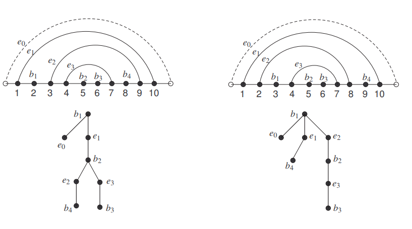
Example 3.17. Assume \(k=4,\, b+1=4, \, \sigma=2, \, \theta=1\), and \(s=3, \, h=1, \, l_e=2, \, g=1\). According to Proposition 3.16, the number of plane trees of the third class is \[\begin{aligned} \frac{1}{3} {3 \choose 1,1,1,0} {2-2 \choose 3-1-1-1}{4-1-1+3-2 \choose 2+3-2} {3-1 \choose 3-1}=2. \end{aligned}\]
The two plane trees and the corresponding RNA secondary structures are shown in Figure 4.
Analogously, we obtain the numbers for the other two classes.
Proposition 3.18. The number \(Q_1(l_e, g)\) of plane trees of the first class in Theorem 3.13 is given by \[\begin{gathered} \frac{ (s-1)! (b+1-h-g)}{h! (g+1)! (s-h-g)! (b+1-s)}\left[(s+1-l_e){s-1-h-g \choose l_e-1-h} + s {s-1-h-g \choose l_e-h} \right]\\ \times {l_e-2 \choose s-h-g-1} {k-g-h(\sigma-1)+s-2 \choose l_e+s-1} {b-1-s(\theta-1) \choose s-1} . \end{gathered} \tag{2}\]
Proposition 3.19. The number \(Q_2(l_e, g)\) of plane trees of the second class in Theorem 3.13 is given by \[\begin{aligned} &\frac{(s-1)! l_e }{h! g! (s+1-h-g)!} {s-h-g \choose l_e-h} {l_e-1 \choose s-h-g-1} \nonumber\\ & \qquad \times {k-g-h(\sigma-1)+s-1 \choose l_e+s} {b-1-s(\theta-1) \choose s-1} . \end{aligned}tag{3}\]
Remark 3.20. We do not know if there is any bio-significance to distinguish partial stacks and right-bulges at the moment. The above three propositions may be useful if the speculated bio-significance is found later.
Finally, it is easy to obtain the following theorem.
Theorem 3.21(Mail Theorem ). The number of RNA secondary structures with \(b\) base pairs, \(k>1\) isolated bases, \(s\) stacks such that each stack contains at least \(\theta\) base pairs and \(h\) hairpin loops such that each hairpin loop has a length at least \(\sigma\) is given by \[\begin{aligned} \sum_{l_e>0} \sum_{g\geq 0} Q_1(l_e, g) +Q_2(l_e, g)+Q_3(l_e,g). \end{aligned} {tag{4}\]
Proof. Note that it is possible for an RNA secondary structure to have no bulge loop. Thus, the summation for the number of bulges is over \(g\geq 0\). The rest is clear and the proof follows. ◻
Remark 3.22 It is possible to express the desired number in Theorem 3.21 in terms of \(Q_3(l_e,g)\) alone, since any RNA secondary structure can be decomposed into isolated segments and components with the leftmost base paired with the rightmost base, and the number of hairpins and stacks are additive across components. Secondly, in Chen, Reidys and Waterman [3], there is a formula computing the number of RNA secondary structures with a given fine parameter specification on hairpins, bulges, interior loops, multiloops, exterior loop and stacks. Certainly, summing over all possible distributions that fix the numbers of hairpins and stacks will also provide us with a formula for the desired number in Theorem 3.21. However, the expression is expected to be more complicated, implying the advantage of the approach in the present paper
The author thanks Christian Reidys for valuable discussion at the early stage of this study. This work was supported by the Anhui Provincial Natural Science Foundation of China (No. 2208085MA02) and Overseas Returnee Support Project on Innovation and Entrepreneurship of Anhui Province (No. 11190-46252022001).
For each \(T \in \mathbb{T}\), we first decompose \(T\) into a forest of small trees according to the following procedure.
i. Set \(i_e=0,\, i_o=0\);
ii. We assume \(\bar{j}<\overline{j+1}\) and any element \(i\in [k]\) is smaller than \(\bar{j}\in [\overline{b+1}]\). In \(T\), find the minimum internal vertex (in terms of its label from \([k]\) and \([\overline{b+1}]\)) whose children are leaves; Remove the small tree determined by \(v\) (i.e., \(v\) and its children), with all labels carried over.
iii. If \(v\) has a label in \([k]\), relabel \(v\) with label \((k+i_e+1)^*\) in the remaining tree (at the original position of \(v\) in \(T\)), and update \(T\) as the resulting tree, and set \(i_e=i_e+1\); If \(v\) has a label in \([\overline{b+1}]\), place a vertex with label \((\overline{s+i_o+1})^*\) in the remaining tree at the original position of \(v\) in \(T\), and update \(T\) as the resulting tree, and set \(i_o=i_o+1\);
iv. If \(T\) is not a small E-tree, go to step ii and continue, the procedure terminates otherwise.
In the end, it is obvious that we obtain \(l_e\) small E-trees and \(s\) small O-trees. Furthermore, we have the following properties.
All small E-trees have roots from \(E\) and all small O-trees have roots from \(O\).
Each odd-level internal vertex induces a starred O-label so there are \(s\) starred O-labels; Each even-level internal vertex, except the root, induces a starred E-label so there are \(l_e-1\) starred E-labels generated.
As the E-blocks are simply carrier over in small E-trees, the property (1) is clear.
Note that the vertices with the labels in \([\overline{h}]\) are internal and appear as the rightmost children of some even-level vertices. Obviously, these vertices induce the labels \(\{(\overline{b+2})^*, \ldots, (\overline{b+1+h})^*\}\) which must appear as the rightmost of children of some small E-trees, whence the property (2).
The last removed small O-tree must have its root as an internal vertex that is a child of the root \(k\). Thus, the corresponding induced starred label \((\overline{b+1+s})^*\) must appear in the small E-tree rooted on \(k\), whence the property (3).
The property (4) is obvious.
Clearly, the set of vertices \(\{\overline{h+1}, \ldots, \overline{h+y}\}\) induce the set of starred labels \[\{ (\overline{b+2+h})^*, \ldots, (\overline{b+1+y+h})^*\}.\]
Since the former are not the rightmost children of any even-level internal vertices, the latter must not appear as the rightmost children of any small E-trees. This leads to the property (5).
Next, we describe how to get back to a tree \(T \in \mathbb{T}\) from a forest \(F\in \mathbb{F}\).
(i) Find a tree in \(F\) with the minimum root such that there is no vertex with a starred label in the tree. If the root \(v\) of the found tree is an \(E\)-vertex, then merge the root with the vertex having the minimum label in the set \(\{ (k+1)^*, (k+2)^*,\ldots, (k+l_e-1)^*\}\) in \(F\), and label the newly generated vertex by the label of \(v\) (and discard the starred label involved). If the root \(v\) of the found tree is an \(O\)-vertex, then merge the root with the vertex having the minimum label in the set \(\{ (\overline{b+2})^*, (\overline{b+3})^*,\ldots, (\overline{b+1+s})^*\}\), and label the newly generated vertex by the label of \(v\). Update \(F\) as the resulting forest of trees.
(ii) iterate (i) until \(F\) becomes a single labelled plane tree \(T\).
Here we remark that a tree without any starred label (sought in step (i)) always exists, because there are in total \(l_e+s\) trees and \(l_e-1+s\) starred labels at the beginning, and later every time we decrease the number of starred E-labels (resp. O-labels) by one, we decrease the number of E-trees (resp. O-trees) by one at the same time. In addition, since the number of E-trees is always one larger than the number of starred E-labels, we eventually obtain an E-tree.
The numbers of even-level internal vertices and odd-level internal vertices in \(T\) are determined by the number of small trees with unstarred roots and are obviously \(l_e\) and \(s\). The number of E-blocks is well preserved in the process and obviously \(s\).
According to the above procedure from \(F\) to \(T\), among small O-trees, the ones with roots from \([\overline{h}]\) will be firstly and respectively merged with the starred labels in \(\{(\overline{b+2})^*, \ldots, \\ (\overline{b+1+h})^*\}\). Since the latter are the rightmost children in some small E-trees, the vertices in \([\overline{h}]\) will be the rightmost children of some even-level internal vertices, and by construction have at least \(\sigma-1\) children all being leaves. Next, analogously, the vertices in the set \(\{\overline{h+1}, \ldots, \overline{h+y}\}\) are the only odd-level internal vertices that are not rightmost children of any even-level vertices and have leaves as children. Since the rest of small O-trees have at least one starred label, they will be odd-level internal vertices that have at least one even-level internal vertex as a child, respectively. Hence, \(T\in \mathbb{T}\).
It should not be hard to verify that the above constructions give a bijection between \(\mathbb{T}\) and \(\mathbb{F}\). This completes the proof.