Graph theoretic problems concerning decompositions and packings have been central in combinatorics, as extensively documented in the foundational texts by Bondy and Murty [5] and Diestel [10]. Two triangles in a graph are said to be edge-disjoint if they do not share any common edge, though they may share at most one vertex. Edge-disjoint triangle packings in graphs arise naturally in several contexts including combinatorial design theory, network reliability, and coding theory.
The study of edge-disjoint triangle packings is intimately connected to Steiner Triple Systems (STS), which represent one of the most extensively studied classes of combinatorial designs [9]. A Steiner Triple System of order \(n\), denoted \(\text{STS}(n)\), is a collection of three-element subsets (called triples) of an \(n\)-element set such that every pair of distinct elements appears in exactly one triple [35]. When represented as a graph, an \(\text{STS}(n)\) corresponds to a perfect decomposition of the complete graph \(K_n\) into edge-disjoint triangles [40].
Furthermore, the classical existence theory for Steiner Triple Systems, established by Kirkman [21] and later proven by Reiss [29], shows that an \(\text{STS}(n)\) exists if and only if \(n \equiv 1\) or \(3 \pmod{6}\). This fundamental result provides a complete characterization of when \(K_n\) can be perfectly decomposed into edge-disjoint triangles. However, when \(n \not\equiv 1, 3 \pmod{6}\), perfect decompositions are impossible, leading naturally to questions about partial triangle packings.
The connection between our enumeration results and classical STS theory runs deeper than mere existence questions. When an \(\text{STS}(n)\) exists, the number of edge-disjoint triangles is exactly \(n(n-1)/6\), and our counting formulas provide a precise enumeration of all possible partial systems with fewer triangles. For the non-STS cases, our results enumerate the complete spectrum of possible triangle packings, extending the classical theory to a comprehensive counting framework.
Building on this foundation, Bryant and Horsley [8] determined the maximum number of edge-disjoint triangles in \(K_n\) for all values of \(n\), corresponding to maximum partial Steiner Triple Systems. Moreover, Wilson’s asymptotic existence theory [41] provides a powerful framework for understanding when partial systems with specified properties exist. For triangle packings, these results establish that the necessary conditions for the existence of \(k\) edge-disjoint triangles in \(K_n\) are also sufficient for sufficiently large \(n\).
Recent advances in hypergraph packing theory have provided new tools for triangle enumeration problems. The asymptotic enumeration of triangle-free graphs by Razborov [28] and the container method developed by Balogh, Morris, and Samotij [2] offer complementary approaches to our exact enumeration techniques.
The computational aspects of triangle packing enumeration connect to the broader area of \(\#P\)-complete counting problems. Valiant [37] established that counting perfect matchings is \(\#P\)-complete, and similar complexity results apply to hypergraph packing problems.
For applications in network analysis, the work of Milo et al. [25] on network motifs demonstrates the practical importance of triangle counting in biological and social networks. The enumeration of small subgraph patterns, including triangles, has applications in understanding network structure and function.
We use the following notation throughout this paper. Let \(T_n\) denote the total number of sets of pairwise edge-disjoint triangles in \(K_n\), including the empty set, and let \(T_n^k\) denote the number of \(k\)-element sets of pairwise edge-disjoint triangles in \(K_n\). The fundamental relationship between these quantities is given by \[\label{eq:fundamental_relation} T_n = \sum\limits_{k=0}^{\mu(n)} T_n^k, \tag{1}\] where \(\mu(n)\) is the maximum number of edge-disjoint triangles possible in \(K_n\). For small values of \(n\), we have the following base cases: \[\begin{aligned} T_3 &= T_3^0 + T_3^1 = 1 + 1 = 2 ,\nonumber\\ T_4 &= T_4^0 + T_4^1 = 1 + 4 = 5 ,\nonumber\\ T_5 &= T_5^0 + T_5^1 + T_5^2 = 1 + 10 + 15 = 26 \nonumber. \end{aligned}\]
Notably, the case of \(K_5\) illustrates the transition from classical STS theory to our enumeration framework. Since \(5 \equiv 5 \pmod{6}\), no \(\text{STS}(5)\) exists, yet we can have at most two edge-disjoint triangles. Our formula \(T_5^2 = 15\) counts all possible pairs of such triangles, providing precise enumeration where classical theory only establishes non-existence of perfect decompositions.
In this paper, we present a recurrence relation for \(T_n\) and derive exact formulas for \(T_n^2\), \(T_n^3\), and \(T_n^4\). The enumeration of \(T_n^2\) relates directly to the classical problem of counting pairs of edge-disjoint blocks in Steiner systems, which has applications in experimental design and error-correcting codes. Our results extend this classical framework to a complete enumeration theory for small triangle packings.
The remainder of this paper is organized as follows. Section 2 establishes the fundamental recurrence relation and develops the asymptotic analysis. Section 3 presents exact enumeration results for double, triple, and quadruple edge-disjoint triangle packings, including small cases. Section 4 discusses computational complexity. Finally, Section 5 discusses applications and concludes with directions for future research.
Before developing our enumeration techniques, we establish the fundamental existence theory underlying our counting results. The existence of \(k\) edge-disjoint triangles in \(K_n\) relates to partial triple systems and their connection to Steiner triple systems. A partial triple system \(\text{PTS}(n,1)\) of order \(n\) with exactly \(k\) triples corresponds to a set of \(k\) edge-disjoint triangles in \(K_n\).
It is well known (see [9], for example) that the maximum number of edge-disjoint triangles in \(K_n\), denoted \(\mu(n)\), is given by \[\label{eq:max_triangles} \mu(n) = \left\lfloor \frac{n(n-1)}{6} \right\rfloor – \delta, \quad \delta = \begin{cases} 1 & \text{if } n \equiv 5 \pmod{6}, \\ 0 & \text{otherwise}. \end{cases} \tag{2}\]
Remark 2.1. The correction term \(\delta\) arises because when \(n \equiv 5 \pmod{6}\), the number of edges \(\binom{n}{2}\) is not divisible by 3, preventing a perfect triangle decomposition. Specifically, \(\binom{n}{2} = \frac{n(n-1)}{2}\), and when \(n \equiv 5 \pmod{6}\), we have \(n(n-1) \equiv 5 \cdot 4 \equiv 2 \pmod{6}\), so \(\binom{n}{2} \equiv 1 \pmod{3}\). Therefore, the maximum number of edge-disjoint triangles is \(\left\lfloor\frac{\binom{n}{2}}{3}\right\rfloor = \frac{n(n-1)}{6} – 1\).
So, the condition for the existence of a \(\text{PTS}(n,1)\) with exactly \(k\) triples is simply \(k \leq \mu(n)\). The connection to Steiner triple systems provides crucial structural insight. An \(\text{STS}(n)\) exists precisely when \(n \equiv 1\) or \(3 \pmod{6}\), achieving the maximum \(\mu(n) = n(n-1)/6\) triangles in a perfect decomposition of \(K_n\). For non-STS cases where \(n \not\equiv 1, 3 \pmod{6}\), perfect decompositions are impossible, but partial systems with \(k < \mu(n)\) triangles can always be constructed. The existence of maximum systems guarantees the existence of all smaller systems by deletion, establishing that any collection of \(k \leq \mu(n)\) edge-disjoint triangles can be realized in \(K_n\).
This existence theory provides the foundation for our enumeration approach. While these results determine when triangle packings exist, our main contribution lies in counting exactly how many such packings are possible for each feasible value of \(k\). Our enumeration results build upon the work of Erdős, Rényi, and Sós [13] on triangle packings and techniques developed by Rödl [30] for general hypergraph packings.
Proposition 2.2. The number of matchings of size \(j\) in the complete graph \(K_n\) is given by \[\label{eq:matchings} M_j(K_n) = \frac{n!}{(n-2j)!2^j j!}. \tag{3}\]
Proof. Choose \(2j\) vertices from \(n\) in \(\binom{n}{2j}\) ways. The number of ways to partition them into \(j\) unordered pairs is \[\frac{(2j)!}{2^j j!}. \nonumber\]
Therefore, \[M_j(K_n) = \binom{n}{2j} \cdot \frac{(2j)!}{2^j j!} = \frac{n!}{(n-2j)!2^j j!}. \nonumber\] ◻
For the next result, given a graph \(G\) and a set of edges \(F \subseteq E(G)\), we let \(T(G \setminus F)\) denote the number of triangle packings in \(G\) that use no edge from \(F\).
Theorem 2.3. For every integer \(n \geq 3\), the number \(T_n\) of edge-disjoint triangle packings in \(K_n\) satisfies the recurrence \[\label{eq:main_recurrence} T_n = T_{n-1} + \sum\limits_{j=1}^{\lfloor(n-1)/2\rfloor} M_j(K_{n-1})T_{n-1}^{(j)}, \tag{4}\] where \(M_j(K_{n-1}) = \frac{(n-1)!}{(n-1-2j)!2^j j!}\) is the number of matchings of size \(j\) in \(K_{n-1}\), and \(T_{n-1}^{(j)}\) denotes the number of triangle packings in \(K_{n-1}\) that avoid a fixed set of \(j\) disjoint edges. The initial values are \(T_0 = T_1 = T_2 = 1\).
Proof. Fix a vertex \(v \in V(K_n)\). We partition all triangle packings of \(K_n\) based on the number \(j\) of triangles containing \(v\), where \(j\) ranges from zero to \(\lfloor(n-1)/2\rfloor\) since each triangle through \(v\) uses two distinct neighbors of \(v\) and these neighbor pairs must be disjoint.
Case 1. If \(j = 0\), then no triangle contains \(v\), so the packing lies entirely in the induced subgraph on the remaining \(n-1\) vertices, which is isomorphic to \(K_{n-1}\). The number of such packings is \(T_{n-1}\).
Case 2. If \(j \geq 1\), then the \(j\) triangles containing \(v\) correspond bijectively to a matching of size \(j\) in \(K_{n-1}\) (the neighborhood of \(v\)). There are \(M_j(K_{n-1})\) such matchings. For any fixed matching \(M\) of size \(j\), the edges of \(M\) are used in the triangles through \(v\) and hence cannot appear in other triangles by edge-disjointness. The remaining triangles must form an edge-disjoint packing in \(K_{n-1} \setminus M\).
Since any two matchings \(M\) and \(M'\) of size \(j\) in \(K_{n-1}\) yield isomorphic graphs \(K_{n-1} \setminus M\) and \(K_{n-1} \setminus M'\) (via the vertex permutation mapping \(M\) to \(M'\)), the number of triangle packings in \(K_{n-1} \setminus M\) depends only on \(j\), not on the specific matching. We denote this quantity by \(T_{n-1}^{(j)}\). Therefore, the number of packings with exactly \(j\) triangles containing \(v\) is \(M_j(K_{n-1}) \cdot T_{n-1}^{(j)}\).
Summing over the two cases yields Eq. (4). ◻
For asymptotic analysis of the recurrence relation established in Theorem 2.3, we require precise control over the recurrence coefficients. The following technical lemma provides the necessary uniform bounds for the matching coefficients that appear in our enumeration.
Lemma 2.4. For \(n \geq 3\) and \(0 \leq j \leq \lfloor(n-1)/2\rfloor\), the number of matchings of size \(j\) in \(K_{n-1}\) satisfies \[M_j(K_{n-1}) = \frac{(n-1)!}{(n-1-2j)!2^j j!} = \frac{(n-1)^{2j}}{2^j j!} \exp(\theta_{n,j}), \nonumber\] where the error term \(\theta_{n,j}\) satisfies \[\theta_{n,j} = -\frac{j(2j-1)}{n-1} + O\left(\frac{j^3}{n^2}\right). \nonumber\]
In particular, for \(j = o(n^{1/2})\), we have \(\theta_{n,j} = o(1)\) and consequently \(M_j(K_{n-1}) \sim \frac{(n-1)^{2j}}{2^j j!}\).
Proof. Starting with the exact formula, we express the factorial quotient as a product. Namely, \[\frac{(n-1)!}{(n-1-2j)!} = \prod_{t=0}^{2j-1} (n-1-t) = (n-1)^{2j} \prod_{t=0}^{2j-1} \left(1 – \frac{t}{n-1}\right). \nonumber\]
Taking logarithms of both sides, we obtain \[\log\left(\frac{(n-1)!}{(n-1-2j)!}\right) = 2j \log(n-1) + \sum\limits_{t=0}^{2j-1} \log\left(1 – \frac{t}{n-1}\right). \nonumber\]
To evaluate the logarithmic sum, we apply the Taylor expansion \(\log(1-x) = -x – \frac{x^2}{2} + O(x^3)\) with \(x = \frac{t}{n-1}\). This yields \[\sum\limits_{t=0}^{2j-1} \log\left(1 – \frac{t}{n-1}\right) = -\frac{1}{n-1}\sum\limits_{t=0}^{2j-1} t – \frac{1}{2(n-1)^2}\sum\limits_{t=0}^{2j-1} t^2 + O\left(\frac{j^3}{n^3}\right). \nonumber\]
Next, we compute the required sums explicitly. We have \[\sum\limits_{t=0}^{2j-1} t = \frac{(2j-1)(2j)}{2} = j(2j-1), \quad \text{and} \quad \sum\limits_{t=0}^{2j-1} t^2 = \frac{(2j-1)(2j)(4j-1)}{6} \leq \frac{8j^3}{3}. \nonumber\]
Substituting these values back into our expression, we find \[\sum\limits_{t=0}^{2j-1} \log\left(1 – \frac{t}{n-1}\right) = -\frac{j(2j-1)}{n-1} + O\left(\frac{j^3}{n^2}\right). \nonumber\]
Exponentiating both sides establishes the desired asymptotic formula. Finally, the bound for \(j = o(n^{1/2})\) follows directly from the fact that \(\frac{j(2j-1)}{n-1} = o(1)\) under this condition. ◻
To understand the dominant contribution to our enumeration, we establish that terms with large \(j\) in the recurrence relation contribute negligibly to the total count.
Theorem 2.5. Let \(J_n = \lfloor n^{2/3} \rfloor\). Then for some constant \(c > 0\), we have \[\sum\limits_{j>J_n} a_{n,j} \cdot T_{n-1-2j} \leq \exp(-cn^{2/3})T_{n-1}, \nonumber\] where \(a_{n,j} = M_j(K_{n-1})\).
Proof. To establish the tail estimate, we return to the recurrence relation from Theorem 2.3 \[T_n = \sum\limits_{j=0}^{\lfloor(n-1)/2\rfloor} a_{n,j}T_{n-1-2j}. \nonumber\] Our goal is to demonstrate that the tail sum for \(j > J_n\) contributes negligibly to the total.
First, we establish an upper bound for the recurrence coefficients. From Lemma 2.4, for sufficiently large \(n\) and \(j > J_n\), we have the bound \[a_{n,j} \leq \frac{(n-1)^{2j}}{2^j j!}. \nonumber\]
Next, we need to control the ratio \(\frac{T_{n-1-2j}}{T_{n-1}}\). To do this, we derive a crude upper bound for \(T_m\). Since triangle packings correspond to choosing edge-disjoint triangles from at most \(\binom{m}{3}\) available triangles, and the maximum number of edge-disjoint triangles is bounded by \(\mu(m) \leq \binom{m}{2}/3\) (due to edge constraints), we obtain \[T_m \leq \sum\limits_{k=0}^{\mu(m)} \binom{\binom{m}{3}}{k} \leq 2^{\binom{m}{3}}. \nonumber\] Consequently, \(\log T_m \leq \binom{m}{3} \leq \frac{m^3}{6}\).
Using this bound, we can estimate the logarithmic ratio as follows \[\log\left(\frac{T_{n-1-2j}}{T_{n-1}}\right) \leq \frac{(n-1-2j)^3 – (n-1)^3}{6} \leq -Cn^2j \nonumber\] for some positive constant \(C\) when \(j = o(n)\). Therefore, we have the exponential decay \[\frac{T_{n-1-2j}}{T_{n-1}} \leq \exp(-Cn^2j). \nonumber\]
Combining our bounds, we can now estimate the tail contribution. Using the bound on \(a_{n,j}\) together with the exponential decay, we find \[a_{n,j} \cdot \frac{T_{n-1-2j}}{T_{n-1}} \leq \frac{(n-1)^{2j}}{2^j j!} \exp(-Cn^2j). \nonumber\]
For \(j > J_n = n^{2/3}\), the exponential term \(\exp(-Cn^2j)\) dominates the polynomial and factorial terms. More precisely, the sum over the tail region satisfies \[\sum\limits_{j>J_n} \frac{(n-1)^{2j}}{2^j j!} \exp(-Cn^2j) \leq \exp(-cn^{2/3}), \nonumber\] for some positive constant \(c\), since the individual terms decay super-exponentially in this range. This completes the proof of the tail estimate. ◻
With these technical tools established, we can now address the main asymptotic result and provide strong evidence for a conjectured asymptotic.
Theorem 2.6. The number \(T_n\) of edge-disjoint triangle packings in \(K_n\) satisfies \[\frac{1}{12}n^2 \log n – Cn^2 \leq \log T_n \leq \frac{1}{4}n^2 \log n + Cn^2 \nonumber,\] for some absolute constant \(C > 0\) and all sufficiently large \(n\).
Proof. We establish elementary upper and lower bounds using direct combinatorial arguments.
For the upper bound, we consider the sequential selection of triangles under edge-disjointness constraints. The maximum number of edge-disjoint triangles is \(\mu(n) = \lfloor\frac{n(n-1)}{6}\rfloor \sim \frac{n^2}{6}\). After selecting \(j\) triangles, the number of available triangles is at most \(\binom{n}{3} – 3j(n-3)\) since each used edge eliminates at most \(n-3\) additional triangles. This gives \[T_n^k \leq \frac{1}{k!} \prod_{j=0}^{k-1} \left[\binom{n}{3} – 3j(n-3)\right]. \nonumber\]
For \(k = \mu(n)\), taking logarithms and using the bound \(\log(1-x) \leq -x\): \[\log T_n^{\mu(n)} \leq \mu(n) \log n + \sum\limits_{j=0}^{\mu(n)-1} \log\left(1 – \frac{18j}{n^2}\right) – \mu(n) \log \mu(n) + O(n^2) \leq \frac{1}{4}n^2 \log n + O(n^2). \nonumber\]
For the lower bound, we use an explicit block construction. Partitioning \([n]\) into \(t = \lfloor n^{1/3} \rfloor\) blocks of size approximately \(b = n^{2/3}\), we form triangles across triples of blocks. Using \(\lfloor b/3 \rfloor\) triangles per triple ensures edge-disjointness. With \(\binom{t}{3} \approx \frac{n}{6}\) independent triples and careful counting of the choices per triple, this construction yields \(\log T_n \geq \frac{1}{12}n^2 \log n – Cn^2\) after parameter optimization. ◻
Corollary 2.7. The number \(T_n\) of edge-disjoint triangle packings in \(K_n\) satisfies \[\log T_n = \Theta(n^2 \log n) \quad \text{as } n \to \infty. \nonumber\]
More precisely, there exist positive constants \(c_1, c_2\) such that \[c_1 n^2 \log n \leq \log T_n \leq c_2 n^2 \log n \nonumber,\] for all sufficiently large \(n\).
Proof. This follows immediately from Theorem 2.6. ◻
The bounds in Theorem 2.6 establish an order of magnitude while Corollary 2.7 proves that triangle packing enumeration grows exponentially with exponent \(\Theta(n^2 \log n)\). However, the gap between the upper bound coefficient \(\frac{1}{4}\) and the lower bound coefficient \(\frac{1}{12}\) suggests that techniques from probabilistic combinatorics, generating function theory, or design enumeration are needed to determine whether the following conjecture is correct.
Conjecture 2.8. The number of edge-disjoint triangle packings in \(K_n\) satisfies \[\log T_n = \frac{1}{6}n^2 \log n + O(n^2) \quad \text{as } n \to \infty. \nonumber\]
The gap between our proven bounds and the conjectured precise asymptotic reflects the genuine difficulty of triangle packing enumeration. While Theorem 2.6 establishes that \(\log T_n = \Theta(n^2 \log n)\), determining the exact coefficient appears to require techniques from probabilistic combinatorics, generating function theory, or design enumeration that go beyond the scope of this paper. Still, the next remark provides strong support for this conjecture, although it should not be counted as mathematical proof.
Remark 2.9. The coefficient \(\frac{1}{6}\) arises naturally from several perspectives. The maximum number of edge-disjoint triangles is approximately \(\frac{n^2}{6}\), suggesting this scale governs the asymptotics. Moreover, by Theorem 2.1 of Pippenger and Spencer [26], the random greedy hypergraph matching process maintains quasirandom structure throughout most of its evolution. This suggests that triangle removal can continue for roughly \(\frac{n^2}{6}\) steps with approximately \(n\) choices per step, yielding \(\exp(\frac{n^2}{6} \log n)\) distinct sequences.
The connection to Steiner triple systems provides additional support. When \(n \equiv 1, 3 \pmod{6}\), perfect triangle decompositions exist, and their enumeration contributes significantly to \(T_n\). Rödl [30] proves that the nibble method produces large partial packings covering almost all edges, while Keevash [19, 20] establishes the existence and asymptotic enumeration of Steiner triple systems. His results imply that there are exponentially many such designs, with an exponent of order \(n^2 \log n\). While the precise coefficient requires careful analysis of his formulas, the \(\frac{1}{6}\) scaling is consistent with the structure of these results, though establishing this connection rigorously remains open.
Having established the general recurrence and asymptotic framework, we now present exact enumeration results for specific values of \(k\), starting with small cases and progressing to more complex configurations. For completeness, we begin with the explicit enumeration for small values of \(n\).
Proposition 3.1. The complete enumeration for small complete graphs is given by \[\begin{aligned} T_3 &= 2 \quad (T_3^0 = 1, T_3^1 = 1) \nonumber,\\ T_4 &= 5 \quad (T_4^0 = 1, T_4^1 = 4) \nonumber,\\ T_5 &= 26 \quad (T_5^0 = 1, T_5^1 = 10, T_5^2 = 15) \nonumber. \end{aligned}\]
Proof. For \(K_3\), there is exactly one triangle, giving \(T_3^0 = 1\) (empty set) and \(T_3^1 = 1\) (the single triangle).
For \(K_4\), there are \(\binom{4}{3} = 4\) triangles, but no two can be edge-disjoint since any two triangles in \(K_4\) must share an edge. Thus \(T_4^0 = 1\), \(T_4^1 = 4\), and \(T_4^k = 0\) for \(k \geq 2\).
For \(K_5\), there are \(\binom{5}{3} = 10\) triangles. Any two triangles can share at most one vertex to be edge-disjoint. Since each triangle uses three vertices and we have only five vertices total, two edge-disjoint triangles must share exactly one vertex. The number of such pairs is \(T_5^2 = 15\), which can be computed by choosing a shared vertex (five ways) and then choosing two pairs from the remaining four vertices (three ways), giving \(5 \times 3 = 15\). ◻
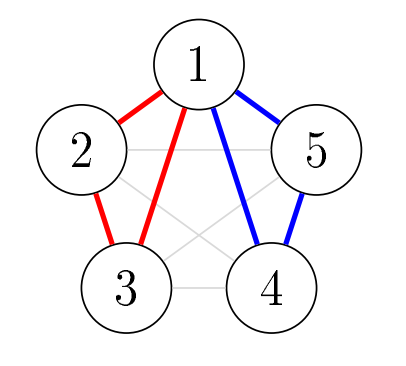
Here, as an example, we illustrate \(T_5^2\), the double edge-disjoint triangle packings in \(K_5\). Let the vertices of \(K_5\) be \(\{1, 2, 3, 4, 5\}\). Since vertex-disjoint triangles would require six vertices, all pairs of edge-disjoint triangles in \(K_5\) must share exactly one vertex. For any fixed vertex \(v\) (say, vertex 1), the triangles containing \(v\) are formed by choosing two vertices from the remaining four. However, two such triangles will be edge-disjoint if and only if the two pairs of vertices chosen are disjoint.
The four remaining vertices can be partitioned into two pairs in exactly three ways:
\(\{\{2,3\}, \{4,5\}\}\) giving triangles \(\{1,2,3\}\) and \(\{1,4,5\}\); see Figure 1 for this case.
\(\{\{2,4\}, \{3,5\}\}\) giving triangles \(\{1,2,4\}\) and \(\{1,3,5\}\)
\(\{\{2,5\}, \{3,4\}\}\) giving triangles \(\{1,2,5\}\) and \(\{1,3,4\}\)
Repeating this process for each of the five vertices gives \(T_5^2 = 5 \times 3 = 15\), a value that is supported by the general formula in Theorem 3.2. Namely, \(T_5^2 = \frac{5 \cdot 4 \cdot 3 \cdot 2 \cdot 1 \cdot 9}{72} = 15\).
Theorem 3.2. For \(n \geq 5\), the number \(T^2_n\) of pairs of edge-disjoint triangles in \(K_n\) is \[T^2_n = \frac{n(n – 1)(n – 2)(n – 3)(n – 4)(n + 4)}{72}.\]
Proof. The result follows by partitioning the count into the cases of vertex-disjoint triangles and triangles sharing exactly one vertex.
Case 1. (Vertex-disjoint triangles).
Choose any 6 vertices out of \(n\) and partition them into two groups of 3. The number of such choices is \[\frac{1}{2!}\binom{n}{6}. \nonumber\]
Case 2. (Triangles sharing exactly one vertex).
For a fixed vertex \(v\) there are \(\binom{n-1}{4}\) ways to choose 4 other vertices and 3 ways to partition these into 2 pairs (which, together with \(v\), form two triangles). Summing over all \(v\) yields \[3n\binom{n-1}{4}. \nonumber\]
Combining these cases, we have \[T_n^2 = \frac{1}{2!}\binom{n}{6} + 3n\binom{n-1}{4} = \frac{n(n-1)(n-2)(n-3)(n-4)(n+4)}{72}. \nonumber\] ◻
This result directly extends classical STS theory by providing exact counts for pairs of edge-disjoint blocks. In the context of \(\text{STS}(n)\) when \(n \equiv 1, 3 \pmod{6}\), this formula counts the number of ways to select 2 triples from the complete system such that they intersect in at most one point.
Definition 3.3. Let \(V\) be a finite labelled vertex set and let \(B\) be a multiset of \(m\) blocks (subsets of \(V\)) of fixed size \(k\) (“\(k\)-blocks”). A configuration is an unordered \(m\)-tuple of \(k\)-blocks drawn from \(\binom{V}{k}\) that satisfies a given combinatorial constraint (e.g. edge-disjointness).
Definition 3.4. Fix a configuration on \(m\) blocks of size \(k\) whose vertex-incidence multiset contains exactly \(N := mk\) vertex-slots (counting multiplicity). The multiplicity profile is the integer partition of \(N\) defined by the multiset of positive vertex-occurrence counts. Equivalently, if the configuration uses exactly \(v\) distinct vertices, and the occurrence-multiplicities of those vertices are \(\mu_1, \ldots, \mu_v\) (positive integers summing to \(N\)), then the multiplicity profile is the vector \((\mu_1, \ldots, \mu_v)\) up to permutation.
The multiplicity profile method reduces the global counting problem to a finite collection of local slot-allocation subproblems, one subproblem per feasible profile.
Proposition 3.5. The total number of configurations on an \(n\)-vertex labelled ground set is \[\sum\limits_{\text{feasible } \mu} \binom{n}{v(\mu)} |A(\mu)|, \nonumber\] where \(v(\mu)\) is the number of distinct vertices used in profile \(\mu\), and \(|A(\mu)|\) is the number of admissible slot allocations for that profile.
Proof. Choose the \(v\)-subset of vertices that will support the configuration in \(\binom{n}{v}\) ways. The number of distinct unordered configurations with multiplicity profile \(\mu\) on a fixed \(v\)-set equals the number of admissible allocations of vertex occurrences to triangle positions, accounting for symmetries. Summing over all feasible profiles yields the formula. ◻
Theorem 3.6. The number \(T_n^3\) of three-element sets of pairwise edge-disjoint triangles in \(K_n\) is \[T_n^3 = 120\binom{n}{6} + 735\binom{n}{7} + 840\binom{n}{8} + 280\binom{n}{9},\nonumber\] for \(n \geq 6\), and \(T_n^3 = 0\) for \(n \leq 5\).
Proof. For \(n \leq 5\), three edge-disjoint triangles require at least six vertices (when all three triangles share a common vertex), so \(T_n^3 = 0\).
For \(n \geq 6\), we use the multiplicity profile method from Definitions 3.3 and 3.4. Here, with \(m = 3\) triangles and \(k = 3\) vertices per triangle, we have \(N = 9\) total vertex-slots. Let \(a(v)\) denote the number of ways to arrange three edge-disjoint triangles on exactly \(v\) vertices. Then \[T_n^3 = \sum\limits_{v=6}^9 a(v)\binom{n}{v}.\nonumber\]
We analyze each case based on the total number of distinct vertices used.
Case 1. (\(v = 9\)).
All triangles are vertex-disjoint. We partition nine vertices into three unordered triples, which gives \[a(9) = \frac{9!}{(3!)^3 \cdot 3!} = 280.\nonumber\]
Case 2. (\(v = 8\)).
Exactly one vertex appears in two triangles. Choose the doubled vertex (eight ways), select four vertices for the two triangles containing it, and partition these into two pairs (three ways). The remaining three vertices form the third triangle. This yields \[a(8) = 8 \cdot \binom{7}{4} \cdot 3 = 840.\nonumber\]
Case 3. (\(v = 7\)).
We must determine all feasible multiplicity profiles for three edge-disjoint triangles using exactly seven vertices.
Claim 1. The only feasible multiplicity profiles for \(v = 7\) are \((3,1^6)\) and \((2^2,1^5)\).
Proof. Since we have \(N = 9\) vertex-slots distributed among \(v = 7\) vertices, the average multiplicity is \(\frac{9}{7} > 1\). By the pigeonhole principle, at least one vertex must appear at least twice. Let \(d\) denote the number of vertices with multiplicity \(\geq 2\). Since each such vertex contributes at least 2 to the total, and the remaining \(7-d\) vertices contribute at least 1 each, we have \[2d + (7-d) \leq 9 \Rightarrow d + 7 \leq 9 \Rightarrow d \leq 2.\]
For \(d = 1\), one vertex has multiplicity \(m \geq 2\), and six vertices have multiplicity 1. This gives \(m + 6 = 9\), so \(m = 3\). This yields profile \((3,1^6)\).
For \(d = 2\), two vertices have multiplicities \(m_1, m_2 \geq 2\), and five vertices have multiplicity 1. This gives \(m_1 + m_2 + 5 = 9\), so \(m_1 + m_2 = 4\). Since \(m_1, m_2 \geq 2\), the only solution is \(m_1 = m_2 = 2\). This yields profile \((2^2,1^5)\). ◻
(a) Profile \((3,1^6)\).
One vertex appears in all three triangles. Choose this vertex (7 ways) and partition the remaining 6 vertices into 3 pairs. This gives \[7 \cdot \frac{6!}{2^3 \cdot 3!} = 105.\nonumber\]
(b) Profile \((2^2,1^5)\).
Two vertices each appear in exactly two triangles. By edge-disjointness, they can appear together in at most one triangle. Choose the doubled pair \(\{a,b\}\) (21 ways), choose a vertex \(x\) to complete triangle \(\{a,b,x\}\) (5 ways), and partition the remaining 4 vertices into pairs for the other triangles (6 ways). This yields \[21 \cdot 5 \cdot 6 = 630.\nonumber\]
Combining subcases gives \(a(7) = 105 + 630 = 735\).
Case 4. (\(v = 6\)).
We determine the unique feasible multiplicity profile.
Claim 2. For \(v = 6\), the unique feasible multiplicity profile is \((2^3,1^3)\).
Proof. With \(N = 9\) vertex-slots distributed among \(v = 6\) vertices, we need integer solutions to \(\sum\limits_{i=1}^6 m_i = 9\) where each \(m_i \geq 1\). Since the minimum total is 6 (all multiplicities equal 1), we need exactly 3 additional slots. The only way to distribute these is to have exactly three vertices with multiplicity 2 and three with multiplicity 1. ◻
For profile \((2^3,1^3)\), edge-disjointness requires that each triangle contains exactly two doubled vertices and one single vertex. Choose three doubled vertices \(\binom{6}{3} = 20\) ways. The triangles have the form \(\{a,b,x\}\), \(\{a,c,y\}\), \(\{b,c,z\}\) where \(\{a,b,c\}\) are doubled and \(\{x,y,z\}\) are single vertices. There are \(3! = 6\) ways to assign single vertices to triangles, yielding \(a(6) = 20 \times 6 = 120\).
The result follows by combining all cases. ◻
The following enumeration involves complex multiplicity profiles that are represented by Figures 2 through 10 in Appendix 5.8. The appendix aids in understanding both the multiplicity profile method and the slot allocation arguments that underlie the proof.
Theorem 3.7. The number \(T_n^4\) of four-element sets of pairwise edge-disjoint triangles in \(K_n\) for \(n \geq 6\) is \[\begin{aligned} \label{eq:quadruple_packing} T_n^4 &= 30\binom{n}{6} + 2100\binom{n}{7} + 25200\binom{n}{8} + 86625\binom{n}{9} \\ &\quad + 116550\binom{n}{10} + 69300\binom{n}{11} + 15400\binom{n}{12}. \nonumber \end{aligned} \tag{5}\]
For \(n \leq 5\), we have \(T_n^4 = 0\).
Proof. For \(n \leq 5\), four edge-disjoint triangles require at least six vertices (when all triangles share a common vertex), so \(T_n^4 = 0\).
For \(n \geq 6\), we apply the multiplicity profile method established above. With \(m = 4\) triangles and \(k = 3\) vertices per triangle, we have \(N = 12\) total vertex-slots. Let \(a(v)\) denote the number of ways to arrange four edge-disjoint triangles on exactly \(v\) vertices. Then \[T_n^4 = \sum\limits_{v=6}^{12} a(v)\binom{n}{v}.\nonumber\]
We analyze each case based on the total number of distinct vertices used by the four triangles, applying slot allocation techniques for each feasible multiplicity profile.
Case 1. (\(v = 12\)). All triangles are vertex-disjoint. Partition twelve vertices into four unordered triples, which gives \[a(12) = \frac{12!}{(3!)^4 \cdot 4!} = 15400.\nonumber\]
Case 2. (\(v = 11\)). By the same constraint analysis as in the previous theorem, profile \((2,1^{10})\) is the unique feasible configuration. Choose the doubled vertex (eleven ways), select four vertices for the two triangles containing it and partition into pairs (\(\binom{10}{4} \times 3 = 210 \times 3\) ways), then partition the remaining six vertices into two triples for the other triangles (ten ways). This yields \[a(11) = 11 \times 210 \times 3 \times 10 = 69300.\nonumber\]
Case 3. (\(v = 10\)). Profile \((2^2,1^8)\) is the unique feasible configuration by constraint analysis. Choose the doubled pair \(\{a,b\}\) (45 ways). Three subcases arise based on their intersection pattern.
(i) \(a\) and \(b\) never appear together. Each appears in exactly 2 triangles. Partition 8 singles into 4 pairs (105 ways), assign 2 pairs to \(a\)-triangles and 2 to \(b\)-triangles (6 ways). This gives \(105 \times 6 = 630\).
(ii) \(a\) and \(b\) appear together in exactly 1 triangle. Choose single for shared triangle (8 ways), choose pair for \(a\)-only triangle (21 ways), choose pair for \(b\)-only triangle (10 ways). This gives \(8 \times 21 \times 10 = 1680\).
(iii) \(a\) and \(b\) appear together in exactly 2 triangles. Choose 2 singles for the shared triangles (28 ways), partition the remaining 6 singles into 2 triples (10 ways). This gives \(28 \times 10 = 280\).
Combining these subcases yields \(a(10) = 45 \times (630 + 1680 + 280) = 116550\).
Case 4. (\(v = 9\)). We systematically determine all feasible multiplicity profiles.
Claim 3. For four triangles on nine vertices, the feasible multiplicity profiles are \((4,1^8)\), \((3,2,1^7)\), and \((2^3,1^6)\).
Proof. Let \(d_k\) denote the number of vertices with multiplicity exactly \(k\). The constraints are \[\begin{aligned} d_1 + d_2 + d_3 + d_4 &= 9,\nonumber\\ d_1 + 2d_2 + 3d_3 + 4d_4 &= 12.\nonumber \end{aligned}\]
Since we have only 4 triangles, multiplicities cannot exceed 4.
If \(d_4 = 1\), then \(d_1 + d_2 + d_3 = 8\) and \(d_1 + 2d_2 + 3d_3 = 8\). Subtracting gives \(d_2 + 2d_3 = 0\), so \(d_2 = d_3 = 0\) and \(d_1 = 8\). This yields profile \((4,1^8)\).
If \(d_4 = 0\) and \(d_3 = 1\), then \(d_1 + d_2 = 8\) and \(d_1 + 2d_2 = 9\). This gives \(d_2 = 1\) and \(d_1 = 7\), yielding profile \((3,2,1^7)\).
If \(d_4 = d_3 = 0\), then \(d_1 + d_2 = 9\) and \(d_1 + 2d_2 = 12\). This gives \(d_2 = 3\) and \(d_1 = 6\), yielding profile \((2^3,1^6)\). ◻
(a) Profile \((4,1^8)\). One vertex appears in all four triangles. Choose this vertex (9 ways), partition the remaining 8 vertices into 4 pairs (105 ways). This gives \(9 \times 105 = 945\).
(b) Profile \((3,2,1^7)\). One vertex \(t\) appears in 3 triangles, another vertex \(d\) appears in 2 triangles. Choose \((t,d)\) ordered (72 ways). Two subcases arise:
(i) \(d\) in 1 \(t\)-triangle + 1 non-\(t\) triangle gives \(\binom{7}{5} \times 5 \times 3 = 315\) per \((t,d)\)
(ii) \(d\) in 2 \(t\)-triangles only gives \(\binom{7}{4} \times \binom{4}{2} = 210\) per \((t,d)\)
This yields \(72 \times (315 + 210) = 37800\).
(c) Profile \((2^3,1^6)\). Three vertices appear twice each. Choose 3 doubled vertices (84 ways). Three structural types arise based on doubled vertices per triangle:
(i) Type \((2,2,2,0)\): Three triangles have 2 doubled vertices each gives \(6 \times 5 \times 4 = 120.\)
(ii) Type \((2,2,1,1)\): Two triangles have 2 doubled vertices each, two have 1, each gives \(540.\)
(iii) Type \((3,1,1,1)\): One triangle has all 3 doubled vertices gives \(15 \times 6 = 90.\)
Combining subcases gives \(a(9) = 945 + 37800 + 63000 = 86625\).
Case 5. (\(v = 8\)). Profile \((2^4,1^4)\) is unique by constraint analysis. Using slot allocation principles similar to previous cases, we obtain \[a(8) = \binom{8}{4} \cdot \frac{12!}{(2!)^4 \cdot (3!)^4} = 70 \cdot \frac{479001600}{16 \cdot 1296} = 25200.\nonumber\]
Case 6. (\(v = 7\)). Profile \((3,2^2,1^4)\) is unique by constraint analysis. The slot allocation gives \[a(7) = 7 \times 15 \times \frac{12!}{3! \cdot 4 \cdot (3!)^4} = 105 \times \frac{479001600}{6 \cdot 4 \cdot 1296} = 2100.\nonumber\]
Case 7. (\(v = 6\)). Profile \((2^6)\) corresponds to a 3-uniform 2-regular hypergraph on six vertices, equivalent to specific 1-factorizations of \(K_6\), yielding \(a(6) = 30\).
Combining all cases yields the stated formula. ◻
Corollary 3.8. As \(n \to \infty\), the number \(T_n^4\) satisfies the asymptotic estimate \[T_n^4 \sim \frac{15400}{12!} n^{12} = \frac{77}{2395008} n^{12}. \nonumber\]
Proof. The expression for \(T_n^4\) in Theorem 3.7 is a linear combination of binomial coefficients \(\binom{n}{k}\) for \(k = 6, 7, \ldots, 12\). Recall that each binomial coefficient \(\binom{n}{k}\) is a polynomial in \(n\) of degree \(k\) given by \[\binom{n}{k} = \frac{n^k}{k!} + O(n^{k-1}). \nonumber\]
Therefore, the dominant term as \(n \to \infty\) comes from the highest degree term, which is \(15400\binom{n}{12}\). We compute \[15400\binom{n}{12} = 15400\left(\frac{n^{12}}{12!} + O(n^{11})\right) = \frac{15400}{12!} n^{12} + O(n^{11}). \nonumber\]
All other terms in the expression are of order \(O(n^{11})\) or lower. Since \(12! = 479001600\), we can simplify \[\frac{15400}{479001600} = \frac{77}{2395008}. \nonumber\]
Thus it follows that \[T_n^4 \sim \frac{15400}{12!} n^{12} = \frac{77}{2395008} n^{12}. \nonumber\] ◻
To confirm the correctness of our closed forms for \(T_n^k\), we carried out computational enumeration of all triangles in \(K_n\) and checked disjointness constraints for small \(n\). Table 1 shows some small \(n\) values. The sequences for \(T_n^k\) with \(k = 2, 3, 4\) have been submitted to and approved in the Online Encyclopedia of Integer Sequences [34] as sequences A381862, A381863, and A054647.
The complexity of counting substructures in graphs traces back to Valiant’s seminal 1979 work establishing the \(\#P\)-completeness hierarchy, where counting perfect matchings in bipartite graphs was shown to be \(\#P\)-complete [37]. The broader framework of \(\#P\)-completeness was developed to capture the computational difficulty of counting problems that correspond to NP decision problems [38].
| \(n\) | \(T(K_n)\) | \(T_n^1\) | \(T_n^2\) | \(T_n^3\) | \(T_n^4\) |
|---|---|---|---|---|---|
| 3 | 2 | 1 | 0 | 0 | 0 |
| 4 | 5 | 4 | 0 | 0 | 0 |
| 5 | 26 | 10 | 15 | 0 | 0 |
| 6 | 271 | 20 | 100 | 120 | 30 |
| 7 | 5596 | 35 | 385 | 1575 | 2310 |
| 8 | 231577 | 56 | 1120 | 10080 | 42840 |
Packing problems in graph theory have their origins in extremal graph theory, particularly the work of Turán [36] and later Erdős and Stone [14] in the 1940s-1960s on forbidden subgraph problems. The specific study of triangle packings emerged from research on decompositions of complete graphs and Steiner triple systems [21, 40].
The algorithmic complexity of packing problems was systematically studied beginning in the 1970s. Karp [18] established the NP-completeness of various packing problems in his foundational 1972 work. The parameterized complexity approach to these problems was developed in the 1990s by Downey and Fellows [11], providing the theoretical framework for understanding when problems become tractable for small parameter values.
For triangle packings specifically, the decision version (determining whether \(k\) edge-disjoint triangles exist) was shown to be NP-complete through reductions from 3-dimensional matching [15]. The complexity of packing problems in planar graphs was studied by Kirkpatrick and Hell [22], though their work focused on vertex-disjoint (rather than edge-disjoint) subgraph packings.
The counting version of triangle packing follows the general pattern established by Valiant [37]: if the decision version of a problem is NP-complete, the corresponding counting version is typically \(\#P\)-complete. This connection was formalized through parsimonious reductions, which preserve the exact number of solutions [33].
Recent applications of triangle counting and packing have emerged in network analysis, where triangular motifs represent fundamental structural units in social networks [39] and biological networks [25]. In computational biology, triangle packings arise in protein interaction network analysis and phylogenetic reconstruction [17].
The enumeration formulas we have derived naturally lead to questions about the computational complexity of computing \(T_n^k\) for fixed \(k\) as a function of \(n\). We consider two fundamental counting problems that arise in triangle packing enumeration. The first concerns computing the number of triangle packings in complete graphs, which corresponds to evaluating the combinatorial functions \(T_n^k\) we have studied. The second addresses the more general problem of counting triangle packings in arbitrary input graphs, where the graph structure itself becomes part of the computational challenge.
Definition 4.1. For integers \(k \geq 0\) and \(v \geq 0\), let \(a_k(v)\) denote the number of sets of \(k\) pairwise edge-disjoint triangles in the complete graph \(K_v\) on labeled vertices \(\{1, 2, \ldots, v\}\).
These coefficients \(a_k(v)\) play a central role in our complexity analysis since they capture the combinatorial essence of triangle packing enumeration independent of the host graph size.
Theorem 4.2. The computational complexity of triangle packing enumeration exhibits the following fundamental dichotomy:
(a) For any fixed constant \(k\), computing \(T_n^k\) can be accomplished in polynomial time \(O(n^{3k})\).
(b) The general problem of computing the number of \(k\)-edge-disjoint triangle packings in an arbitrary graph \(G\) is \(\#P\)-complete when \(k\) is part of the input.
(c) For fixed \(k\), the coefficients \(a_k(v)\) can be precomputed in time \(O(v^{3k})\) for all relevant values of \(v\), after which \(T_n^k\) can be evaluated in \(O(k^2)\) arithmetic operations using the expansion \[T_n^k = \sum\limits_{v=v_{\min}}^{3k} a_k(v)\binom{n}{v}, \nonumber\] where \(v_{\min}\) is the minimum number of vertices required to support \(k\) edge-disjoint triangles.
Proof. The proof demonstrates each aspect of the complexity dichotomy through different algorithmic and reduction techniques.
For the polynomial-time result when \(k\) is fixed, we employ direct enumeration. The complete graph \(K_n\) contains exactly \(\binom{n}{3}\) triangles, so there are \(\binom{\binom{n}{3}}{k}\) possible \(k\)-element subsets to consider. Since \(\binom{n}{3} = O(n^3)\) and \(k\) is constant, this gives \[\binom{\binom{n}{3}}{k} = O\left(\frac{(n^3)^k}{k!}\right) = O(n^{3k}) \nonumber,\] candidate sets. Each candidate can be tested for edge-disjointness in \(O(k^2)\) time by examining the edges used by the \(k\) triangles. Therefore, the total running time is \(O(n^{3k})\) for fixed \(k\).
The \(\#P\)-completeness result for arbitrary \(k\) follows from a parsimonious reduction from \(\#3D\)-Matching, a canonical \(\#P\)-complete problem. Given a 3-uniform hypergraph \(H = (X \cup Y \cup Z, E)\) with \(|X| = |Y| = |Z| = m\), we construct a graph \(G_H\) that encodes the matching constraints through a gadget-based design.
The construction proceeds as follows. For each element \(p \in X \cup Y \cup Z\), we introduce two vertices \(p_L\) and \(p_R\) connected by an element edge \((p_L, p_R)\). For each hyperedge \(e = (x, y, z) \in E\), we add a gadget vertex \(u_e\) and connect it to all six vertices \(x_L, x_R, y_L, y_R, z_L, z_R\). This creates exactly three triangles within each gadget: \(\{u_e, x_L, x_R\}\), \(\{u_e, y_L, y_R\}\), and \(\{u_e, z_L, z_R\}\).
The key insight is that element edges serve as exclusive resources. Two triangles from different gadgets that both attempt to use the same element edge \((p_L, p_R)\) share that edge and cannot both appear in an edge-disjoint packing. This constraint structure exactly mirrors the disjointness requirements of 3D-matching.
To establish a bijection, we employ a canonicalization scheme. We fix a total ordering on all elements in \(X \cup Y \cup Z\) and designate, for each hyperedge \(e = (x, y, z)\), the triangle corresponding to the smallest element among \(\{x, y, z\}\) as the canonical triangle for gadget \(e\). This ensures that each perfect 3D-matching in \(H\) corresponds to exactly one set of \(m\) edge-disjoint canonical triangles in \(G_H\), and conversely.
The reduction preserves the count exactly (parsimoniousness), runs in polynomial time, and reduces a \(\#P\)-complete problem to triangle packing enumeration, establishing \(\#P\)-completeness for the general case.
For the precomputation approach, we observe that any set of \(k\) edge-disjoint triangles uses between \(v_{\min}\) and \(3k\) vertices, where \(v_{\min}\) is the smallest integer such that \(K_{v_{\min}}\) can support \(k\) edge-disjoint triangles. The number of such triangle packings in \(K_n\) can be expressed as \[T_n^k = \sum\limits_{v=v_{\min}}^{3k} a_k(v)\binom{n}{v} \nonumber,\] since we choose \(v\) vertices from \(n\) in \(\binom{n}{v}\) ways and then count the edge-disjoint packings on those \(v\) vertices.
Each coefficient \(a_k(v)\) can be computed by enumerating all \(\binom{\binom{v}{3}}{k} = O(v^{3k})\) possible \(k\)-subsets of triangles in \(K_v\) and testing for edge-disjointness. Since there are only \(O(k)\) relevant values of \(v\), the total precomputation time is \(O(v^{3k})\). Once these coefficients are known, evaluating the sum requires computing \(O(k)\) binomial coefficients, each computable in \(O(k)\) time, yielding \(O(k^2)\) total arithmetic operations. ◻
This complexity dichotomy exemplifies a fundamental pattern in parameterized complexity theory. When the parameter \(k\) is fixed and small, the problem becomes tractable through exhaustive enumeration within the constrained search space. However, when \(k\) grows as part of the input, the exponential dependence on \(k\) renders the problem intractable, aligning with the \(\#P\)-complete classification.
The precomputation strategy offers practical benefits for applications where multiple evaluations of \(T_n^k\) are needed for the same value of \(k\) but different values of \(n\). By separating the combinatorially intensive computation of \(a_k(v)\) coefficients from the polynomial evaluation of the resulting sum, we achieve significant computational savings in repeated computation scenarios.
These results provide a complete characterization of the computational landscape for triangle packing enumeration, establishing both the theoretical boundaries of tractability and practical algorithmic approaches for efficient computation within those boundaries.
We have established both exact enumeration formulas for small triangle packings and asymptotic bounds for the total growth rate. The exact formulas for \(T_n^2\), \(T_n^3\), and \(T_n^4\) extend classical Steiner Triple System theory and provide practical tools for counting edge-disjoint triangle configurations. Our main asymptotic contribution is that \(\log T_n = \Theta(n^2 \log n)\). This establishes that triangle packing enumeration grows exponentially with a quadratic logarithmic exponent. However, the gap between our proven bounds (\(\frac{1}{12} \leq \text{coefficient} \leq \frac{1}{4}\)) and the conjectured precise coefficient \(\frac{1}{6}\) indicates the genuine difficulty of triangle packing enumeration.
Our enumeration results for edge-disjoint triangle packings extend classical Steiner Triple System theory and have applications across several domains in combinatorics and applied mathematics.
In telecommunications networks, triangular topologies provide natural redundancy structures for fault tolerance [16]. Consider a metropolitan area network connecting 8 major switching centers. Using our result \(T_8^2 = 1{,}120\), network planners can evaluate 1,120 distinct ways to establish two triangular protection rings among these centers. For instance, one configuration might use triangles \(\{A, B, C\}\) and \(\{D, E, F\}\) where centers \(A, B, C\) form one protection ring and centers \(D, E, F\) form another, with centers \(G\) and \(H\) serving as backup nodes. If the direct link \(A \leftrightarrow B\) fails, traffic can route through \(C\), while the second triangle provides independent redundancy for the remaining network segments.
In submarine cable networks, consider a transatlantic system with 12 landing points across North America, Europe, and intermediate islands. Our formula \(T_{12}^4 = 1{,}154{,}217{,}930\) indicates over one billion ways to arrange four edge-disjoint triangular cable configurations. A practical example involves triangles connecting \(\{\text{New York}, \text{London}, \text{Reykjavik}\}\), \(\{\text{Boston}, \text{Dublin}, \text{Faroe Islands}\}\), \(\{\text{Miami}, \text{Madrid}, \text{Azores}\}\), and \(\{\text{Montreal}, \text{Amsterdam},\\ \text{Greenland}\}\). Each triangle provides a complete backup routing system, and the edge-disjoint property ensures that no two triangles share the same physical cable link [27].
Triangle packings relate directly to constant-weight error-correcting codes [24]. Consider a data transmission system using our \(T_8^3 = 10{,}080\) result. We construct a constant-weight code with 10,080 codewords, each of length \(\binom{8}{2} = 28\) bits and weight 9 (representing three triangles with three edges each). The edge-disjoint property guarantees minimum Hamming distance 6 between any two codewords.
For example, codeword \(c_1\) might correspond to triangles \(\{1, 2, 3\}\), \(\{4, 5, 6\}\), \(\{7, 8, 1\}\) represented as a 28-bit vector where positions correspond to edges \((i, j)\) with \(i < j\). The bits at positions \((1, 2)\), \((1, 3)\), \((2, 3)\), \((4, 5)\), \((4, 6)\), \((5, 6)\), \((7, 8)\), \((7, 1)\), \((8, 1)\) are set to 1, while all others are 0. Any other codeword \(c_2\) representing three different edge-disjoint triangles will differ in at least 6 positions, enabling detection and correction of up to 2 bit errors during transmission [42].
In pharmaceutical research, consider a clinical trial testing 7 experimental drugs across multiple treatment centers. Using our formula \(T_7^2 = 385\), researchers have 385 ways to design a two-center study where each center tests exactly three drugs in triangular interaction patterns.
A specific design might assign center A to test drugs \(\{X, Y, Z\}\) in all pairwise combinations, while center B tests \(\{U, V, W\}\) similarly, with drug \(T\) serving as a common control. The edge-disjoint property ensures that no drug pair is tested at both centers, eliminating inter-center confounding effects. This design allows researchers to estimate six drug interactions at center A, six at center B, while maintaining statistical independence between centers. The total of 385 possible designs enables optimization based on patient demographics, geographic factors, or regulatory constraints [1].
In agricultural field trials, consider testing 6 fertilizer combinations across experimental plots. Our result \(T_6^2 = 100\) provides 100 ways to arrange two triangular block designs. One arrangement might use triangular plots testing fertilizers \(\{\text{NPK-high}, \text{Organic}, \text{Control}\}\) in the north field and \(\{\text{NPK-low}, \text{Compost}, \text{Biochar}\}\) in the south field. The triangular geometry ensures each fertilizer pair appears exactly once per field, while edge-disjointness prevents fertilizer interactions from confounding results across fields [32].
In online social platforms, triangular closure patterns represent fundamental community structures [39]. Consider analyzing a social network of 10 users where our result \(T_{10}^3 = 86{,}625\) indicates 86,625 ways to identify three non-overlapping triangular friend groups.
A practical example involves users \(\{\text{Alice}, \text{Bob}, \text{Carol}\}\) forming one tight-knit group where all three are mutual friends, \(\{\text{David}, \text{Eve}, \text{Frank}\}\) forming another group, and \(\{\text{Grace}, \text{Henry}, \text{Ivan}\}\) forming a third group, with user Jack remaining unaffiliated. This configuration helps social media algorithms understand community boundaries for targeted advertising, content recommendation, and friend suggestions. The edge-disjoint property ensures that identified communities have minimal overlap, providing cleaner segmentation for marketing analytics [23].
Twitter’s community detection algorithms could use this enumeration to identify non-overlapping influential clusters. For instance, among 9 political commentators, one triangle might include \(\{\text{Progressive-A}, \text{Progressive-B}, \text{Progressive-C}\}\), another \(\{\text{Conservative-A},\\ \text{Conservative-B}, \text{Conservative-C}\}\), and a third \(\{\text{Moderate-A}, \text{Moderate-B}, \text{Moderate-C}\}\). The 735 possible configurations (from \(T_9^3 = 735\)) help algorithms optimize echo chamber detection and cross-community bridge recommendations [12].
In protein interaction networks, triangular motifs represent functional modules [25]. Consider analyzing a metabolic pathway involving 8 key enzymes. Our formula \(T_8^2 = 1{,}120\) indicates 1,120 ways to identify two non-overlapping triangular functional modules.
A specific example involves enzymes \(\{E_1, E_2, E_3\}\) forming a glycolysis regulation triangle where each enzyme pair exhibits strong co-expression, while enzymes \(\{E_4, E_5, E_6\}\) form a lipid synthesis triangle. Enzymes \(E_7\) and \(E_8\) serve as connecting hubs between pathways. This decomposition helps biologists identify drug targets: inhibiting any enzyme in the glycolysis triangle affects glucose metabolism, while targeting the lipid triangle impacts fat synthesis, with minimal cross-pathway interference due to edge-disjointness [17].
In SARS-CoV-2 research, consider 7 viral proteins where \(T_7^2 = 385\) represents possible ways to identify two triangular interaction modules. One triangle might involve \(\{\text{Spike},\\ \text{NSP1}, \text{NSP2}\}\) representing entry mechanisms, while another involves \(\{\text{NSP12}, \text{NSP13},\\ \text{NSP14}\}\) representing replication machinery. This modular decomposition guides multi-target drug design strategies.
In cloud computing, consider allocating virtual machines across 6 physical servers using our result \(T_6^2 = 100\). Each configuration represents two triangular server clusters where servers within each triangle share workload balancing responsibilities.
A practical deployment might cluster servers \(\{S_1, S_2, S_3\}\) for CPU-intensive applications and \(\{S_4, S_5, S_6\}\) for memory-intensive applications. The triangular arrangement ensures that if server \(S_1\) fails, applications can migrate to either \(S_2\) or \(S_3\) within the same cluster, maintaining performance characteristics. The edge-disjoint property prevents resource conflicts between clusters, ensuring predictable performance isolation. Among the 100 possible configurations, cloud providers can optimize based on power consumption, network topology, or maintenance schedules [3].
In manufacturing scheduling, consider a factory with 9 production lines where \(T_9^3 = 735\) represents ways to form three triangular production cells. One configuration might assign lines \(\{L_1, L_2, L_3\}\) to automotive parts, \(\{L_4, L_5, L_6\}\) to aerospace components, and \(\{L_7, L_8, L_9\}\) to consumer electronics. Within each triangle, the three production lines can substitute for each other during maintenance or high-demand periods. The edge-disjoint property ensures that no production line serves multiple product categories simultaneously, maintaining quality control and reducing setup times [7].
In threshold secret sharing schemes, consider 8 participants where our formula \(T_8^2 = 1{,}120\) provides 1,120 ways to establish two independent triangular access structures. In one configuration, participants \(\{\text{Alice}, \text{Bob}, \text{Carol}\}\) can jointly reconstruct secret \(S_1\), while participants \(\{\text{Dave}, \text{Eve}, \text{Frank}\}\) can reconstruct secret \(S_2\). Participants George and Helen serve as trustees with special roles.
The edge-disjoint property ensures information-theoretic security: knowledge of participants in one triangle provides no information about the other secret. This design supports scenarios like nuclear launch codes where two independent triangular groups must agree simultaneously. The 1,120 possible configurations allow security designers to optimize based on geographic distribution, organizational hierarchy, or operational requirements [35].
For future directions, we note that the multiplicity profile method presented here extends beyond triangle packings to general hypergraph enumeration problems. Recent advances in hypergraph regularity theory [31] suggest that similar counting techniques may apply to \(r\)-uniform hypergraphs for \(r > 3\).
The extension to random graphs \(G(n, p)\) presents particularly interesting challenges. For triangle packings in random graphs, the threshold behavior near \(p = \Theta(n^{-1/2})\) determines when large triangle packings first become possible [4]. Our enumeration techniques, combined with martingale methods from probabilistic combinatorics, could provide precise counts for the expected number of triangle packings of size \(k\) in random graphs.
Another promising direction involves studying triangle packings in geometric graphs, where vertices are points in Euclidean space and edges connect nearby points [6]. The geometric constraints create additional structure that may lead to more efficient enumeration algorithms and refined asymptotic estimates.
The author thanks the anonymous referees for their careful reading and helpful suggestions that improved the presentation of this work.
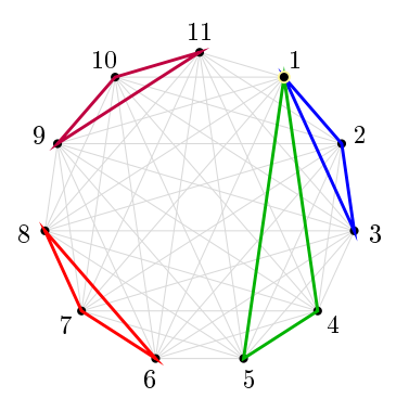
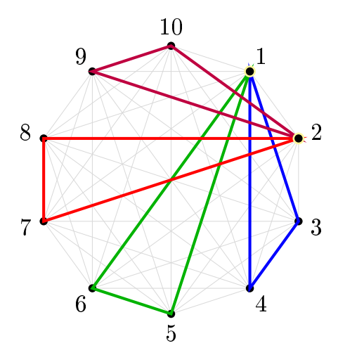
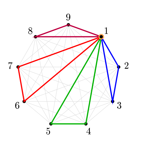
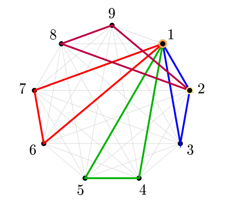
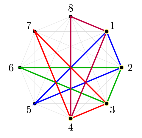
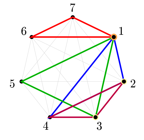
This appendix illustrates all multiplicity profile cases for 4-triangle edge-disjoint packings as proved in Theorem 3.7. Each configuration is drawn within the complete graph \(K_v\) of the relevant order \(v\) and each triangle uses a different color to distinguish the four triangles in each packing.
| \(v\) | \(a(v)\) | Profile Type | Description |
|---|---|---|---|
| 12 | 15400 | \((1^{12})\) | Four vertex-disjoint triangles |
| 11 | 69300 | \((2, 1^{10})\) | One vertex doubled |
| 10 | 116550 | \((2^2, 1^8)\) | Two vertices doubled each |
| 9 | 86625 | Multiple | \((4,1^8)\), \((3,2,1^7)\), \((2^3,1^6)\) |
| 8 | 25200 | \((2^4, 1^4)\) | Four vertices doubled each |
| 7 | 2100 | \((3, 2^2, 1^4)\) | Complex overlapping |
| 6 | 30 | \((2^6)\) | Maximum overlap |
The complete formula is: \[T_n^4 = 30\binom{n}{6} + 2100\binom{n}{7} + 25200\binom{n}{8} + 86625\binom{n}{9} + 116550\binom{n}{10} + 69300\binom{n}{11} + 15400\binom{n}{12}.\]