
The rapid development of simulation, algorithms and mathematics has triggered the rapid progress of lightweighting technology, and lightweighting has spread from automotive, aerospace, aviation and other fields to the traditional manufacturing field, and has become an important development direction in the field of mechanical manufacturing [5, 31, 24]. The design of mechanical components is a comprehensive consideration of structure, material, process and other factors to meet the requirements of its function, structure and performance [26, 22]. Theoretically, the design of a component to reach the limit of lightweighting should be to make the component in the working state, all the local performance is close to or reached the limit performance of the state, there is no redundancy in the structural design [3, 34, 25, 8]. That is, the theoretical limit reached by the lightweight design of mechanical components is that the component in the working state, all of its local performance is played to the extreme [18, 9]. However, the current design of mechanical components is far from involving this issue, which presents a new challenge to mechanical design.
Lightweighting is essentially a multidisciplinary design optimization problem. At present, the optimal design of mechanical equipment and components structure is mainly through the topology optimization technology to optimize the shape and size, design to meet the use requirements and lightweight structure [29, 16]. Structural dimensions generally refer to the external dimensions of the body and components, plate thickness, cross-sectional shape dimensions, joint dimensions and other parameters, which are used as the design variables to construct and optimize the structure with the objective function of minimizing the structural mass under the conditions of stiffness, strength, vibration, energy absorption, safety, fatigue and other conditions that meet the various working conditions [13, 27, 12, 10]. The lightweighting of mechanical structures using topology optimization method overcomes the subjective dependence on human in traditional design, especially in the lightweighting of industrial components, which is widely used [28, 7, 11]. In addition, the topology optimization method can realize the lightweight structure optimization design concept closer to “no performance redundancy”, so that the design of mechanical components is closer to the limit of lightweight, which is the breakthrough and development of the lightweight design of machinery and its concept [19, 23, 17, 35]. It provides a possibility for further realizing the design of the best working capacity state embodied by the reasonable matching of the local performance of the parts.
Mechanical optimal design is the use of simulation, algorithms and mathematical means to establish an optimization model to meet the design requirements, the use of computer analysis and calculation, so that the design of mechanical parts and components in certain constraints, through the appearance, shape, structure, quality, cost, load-bearing capacity, power characteristics of the adjustment of the design of machinery and equipment structure to optimize [14, 38]. Hu et al. [6] showed that topology optimization of mechanical structures can be used to obtain excellent mechanical equipment performance by reasonably arranging the equipment materials in the engineering design stage, and combined with the finite element analysis method to calculate the mechanical structures under different topology optimization methods to effectively reduce the redundant mechanical structures in order to improve the performance of mechanical equipment. Pang & Fard [21] topology-optimized design model for reducing the weight of bell cranks to achieve lightweight and structurally robust road racing car design using weights as the objective function and structural stiffness and strain energy as the optimization constraints. Zhang et al. [36] designed a multi-objective topology optimization method and applied it to improve the topology layout optimization of automobile wheels and performed crash simulations under impact load conditions, and found that the method effectively improved the impact resistance of wheels made of lightweight materials. Wang et al. [32] applied the topology optimization method of major structural components to the robot integration design and established a meta-model of the robot mass-stiffness interrelationship through finite element analysis and virtual joint method to achieve lightweight robot integration design. Xue et al. [33] proposed a hybrid topology optimization method (SIMP-GA) fusing SIMP (solid isotropic material with penalization) method and genetic algorithm, which significantly improves the computational efficiency of structural design and ensures the connectivity of the structure, and provides an effective way for the lightweight design of machinery and equipment structure. Zhou et al. [37] examined the anisotropic topology optimization design method applicable to heavy UAVs to promote the automated design of large-scale three-dimensional variable-axis multi-condition lightweight composite structures, which is conducive to the excellent performance of heavy UAVs even under complex multi-load conditions. Long et al. [2] emphasized that topology optimization is an effective method to obtain a lightweight structure that meets the structural strength requirements, which can provide a reference for the lightweight design of a miniature flapping wing vehicle (FMAV) by establishing topology optimization models with different loads and constraints. Orme et al. [20] introduced additive manufacturing constraints for structural minimization in the topology optimization algorithm, and successfully realized the lightweight topology optimization design of space vehicles through design exploration and numerical computation. It can be seen that mechanical optimization design is an important method for mechanical equipment to achieve lightweight, and it is very crucial to improve the design quality of mechanical equipment and components, and shorten the role of the research and development cycle.
In this paper, an algebraic topology approach is used for lightweight design of automated mechanical equipment structures. Mathematical formulas are used to describe the mechanical equipment topology optimization problem, and a linear programming algorithm is used to solve it. Take the bridge crane as an example, the topology optimization of its main girder structure is carried out. The corresponding design variables, objective functions and constraints are determined according to the Crane Design Manual. Based on the homotopy group algebraic topology tool, the geometric structure of the topological space is transformed into a group, and the improved Memetic algorithm is used to solve the parameters. The mass, strength and stiffness of the main girder structure before and after optimization are analyzed statically, and the modal dynamic analysis of the main girder structure is carried out for each order of frequency, so as to judge the effect of structural lightweighting.
To effectively apply lightweight design principles, it is essential to establish a theoretical foundation based on algebraic topology, which provides the tools to model and analyze structural connectivity.
Algebraic topology is a branch of mathematics that combines algebraic and topological concepts to study structural similarity [4]. It is mainly concerned with how to inscribe and categorize topological spaces by algebraic structures and how to use topological concepts to study algebraic structures.
Topological space is a fundamental concept in mathematics used to study the structure and properties of spaces. In a topological space, the set of points and the sets of these points have certain structural relations between them, and this relation will be introduced in open sets to describe it [30]. The topological space is defined as follows:
Consider a set of ordered pairs \(\left(X,\tau \right)\), where \(X\) is a set and \(\tau\) is a cluster of subsets of \(X\), when the following properties are satisfied:
1) The empty set and \(X\) belong to \(\tau\).
2) The union of any number of elements in \(\tau\) still belongs to \(\tau\).
3) The intersection of a finite number of elements in \(\tau\) still belongs to \(\tau\).
Then this ordered pair \(\left(X,\tau \right)\) is a topological space, \(\tau\) is a topology of \(X\), and the elements of \(\tau\) are called open sets. Here is a concrete example, assuming \(X=\left\{a,b,c\right\}\), then \(\tau _{1} =\left\{\emptyset ,\left\{a\right\},\left\{a,b,c\right\}\right\}\) is a valid topology on \(X\), while \(\tau _{2} =\left\{\emptyset ,\left\{a\right\},\left\{b\right\},\left\{c\right\}\left\{a,b,c\right\}\right\}\) is not, since \(\left\{a\right\}\cup \left\{b\right\}=\left\{a,b\right\}\) is not an element of \(\tau\). Then \(\left(X,\tau _{2} \right)\) is a topological space. From this, it can be seen that only one topological space is constructed here, and in fact multiple topological spaces can be constructed depending on \(X\) and differently on \(\tau\).
Homotopy groups provide a mathematical basis for optimization models as a central tool for characterizing the “connectivity” and “hole structure” of topological spaces.
Suppose that there is a topological space \(X\), and that the \(n\)-dimensional homotopy group \(H_{n} (X)\) consists of all \(n\)-dimensional chains generated by mapping \((n+1)\) for the boundary of a simplex in \(X\) to a \(n\)-dimensional simplex. One of the important features of homotopy groups is that they are closed to group operations if \(a\) and \(b\) are elements in \(H_{n} (x)\). Homotopy groups can be computed by chaining and boundary mapping with the formula: \[\label{GrindEQ__1_} H_{n} (x)=\ker \left(\partial :C_{n} (x)\to C_{n-1} (X)\right)/im\left(\partial :C_{n+1} (X)\to C_{n} (X)\right) , \tag{1}\] where \(C_{n} (X)\) is the \(n\)-dimensional simplex complexity of \(X\) and \(\partial\) is the boundary mapping, which maps \(n\)-dimensional chains to \((n-1)\)-dimensional chains.
The current large-scale machinery manufacturing industry is mainly through the selection of high-quality materials, improve the level of product design and the use of advanced technology and other three main ways to lightweight mechanical equipment components, which is more obvious in the automobile manufacturing industry, aerospace and aviation technology, as well as military and defense fields. This is mainly due to the lightweight mechanical equipment components to improve the improvement of mechanical equipment components of the advanced and stability, thereby ensuring the safety and reliability of the components when used. It can be seen that the application of lightweight mechanical equipment components technology, in order to improve the design level of mechanical components and production technology is of great significance at the same time, but also in energy saving and environmental protection, improve the utilization rate of raw materials, and increase the efficiency of the product and so on play a great role.
Among the ways to realize lightweighting, structural optimization design is the most basic and commonly used means, i.e., to reduce the weight of the structure as much as possible under the premise of meeting the structural strength, stiffness and other conditions. Therefore, structural optimization design is often used to design new products, improve existing structures, and seek safe and economical structural forms, and has now become an indispensable tool in modern design methods.
According to the different classification of design variables, structural optimization can be divided into three levels: size optimization, shape optimization, and topology optimization, and each level of optimization corresponds to a different design stage according to the degree of difficulty in solving the three levels. Because the topology optimization design method can provide the designer with a conceptual design model at the initial stage of engineering design problems, and can obtain the structural form with the optimal material distribution, so compared with the first two, it can obtain greater economic benefits, and the quality of the topology directly affects the quality of the final optimization plan [15].
The main object of study in the optimal design of structural topology is the continuum, and the results of the optimal solution for topology optimization need to describe the specific material characteristics in the continuum structure. This is to make the topological problem of seeking the optimal solution transformed into the problem of seeking the optimal distribution of materials in a specific region. The continuum structure is discretized through the finite element idea. The problem of its material presence or absence is discussed, i.e. here the problem of density 0 and 1. 0 represents the removal of material and 1 represents the retention of material. The overall density distribution of all the cells is continuously calculated and finally the retained density distribution forms the structure which is the optimal force transfer path for the structure.
OptiStruct is a finite element analysis and topology-optimization solver within Altair HyperWorks, used to conceptualize and refine structural designs. Depending on design requirements, it supports optimization of static, modal, and other performance measures. A generic structural optimization model addressed by OptiStruct can be written as
\[\label{eq:optistruct} \left\{\begin{aligned} & \min_{X \in \mathbb{R}^n} && f(X) = f(x_1,\ldots,x_n) \\[2pt] & \text{s.t.} && g_j(X) \le 0, \qquad j=1,\ldots,m, \\[-2pt] & && h_k(X) = 0, \qquad k=1,\ldots,m_h, \\[-2pt] & && x_i^{L} \le x_i \le x_i^{U}, \qquad i=1,\ldots,n . \end{aligned}\right. \tag{2}\]
The objective function \(f(X)\), constraint functions \(g(X)\) and \(h(X)\) are the corresponding results obtained from finite element analysis.
In order to improve the static, dynamic performance of the mechanical equipment structure and to achieve lightweight design, topology optimization design under constraints is achieved by defining different optimization objectives. Static and dynamic performance in FEA refers to the mathematical indexes of static stiffness and modal frequency and the volume fraction and mass of the structure, which are defined as optimization objectives and constraint functions according to different requirements.
The mathematical model, with cell densities as design variables and structural volume as the objective, is \[\label{eq:model} \left\{\begin{aligned} & \min_{\,\{x_{i,j}\}} && V(x) \;=\; \sum_{i=1}^{m}\sum_{j=1}^{n} v_{i,j}\, x_{i,j} \\[2pt] & \text{s.t.} && C(x) \;=\; \beta\, C_{0}, \\[-2pt] & && K(x)\,U \;=\; F, \\[-2pt] & && x_{i,j} \in \{0,1\}, \qquad i=1,\dots,m,\; j=1,\dots,n. \end{aligned}\right. \tag{3}\] Here, \(x_{i,j}\) denotes the (binary) cell density of the \(j\)-th cell in the \(i\)-th subdomain, \(v_{i,j}\) is the corresponding cell volume, \(V(x)\) is the total structural volume, \(C(x)\) is the structural compliance (flexibility) with baseline \(C_{0}\) and scaling factor \(\beta\), \(K(x)\) is the stiffness matrix, \(U\) the displacement vector, and \(F\) the external load vector. \(V_{0}\) denotes the pre-optimization volume.
In the mathematical model, \(x_{j}\) is discrete between 0 and 1, which makes optimization impossible. So, it is assumed to be a continuous variable i.e: \[\label{GrindEQ__6_} 0\le x_{\min } \le x_{j} \le 1,\left(j=1,2,\ldots ,n\right) , \tag{4}\] where \(x_{\min }\) is the smallest material unit density value.
In practice such units do not exist, and in order to avoid the generation of such units and to make the iterative calculations fast, a penalty factor is introduced so that it restricts the intermediate density units. In this paper, the SIMP interpolation method is used, assuming that the establishment of a relational equation for the existence of the setup variable and the elastic modulus allows the calculation to proceed.
Mathematical model for modal-frequency topology optimization: \[\label{eq:modal_topopt} \left\{\begin{aligned} & \max_{\{x_j,\Phi_i,\;\omega_i\}}\quad \omega_i^2(x) \;=\; \frac{\Phi_i^{\mathsf T} K(x)\, \Phi_i}{\Phi_i^{\mathsf T} M(x)\, \Phi_i} \\[3pt] & \text{s.t.}\quad \bigl(K(x) – \omega_i^{2} M(x)\bigr)\,\Phi_i = 0, \\[2pt] & \hphantom{\text{s.t.}}\quad \sum_{j=1}^{n} v_j\, x_j \;\le\; f\, V_0, \\[2pt] & \hphantom{\text{s.t.}}\quad x_{\min} \le x_j \le 1,\qquad j=1,\ldots,n . \end{aligned}\right. \tag{5}\] Here, \(\omega_i\) is the \(i\)-th natural (intrinsic) frequency, \(\Phi_i\) the corresponding eigenvector, \(K(x)\) and \(M(x)\) the stiffness and mass matrices, respectively; \(v_j\) is the volume associated with element \(j\), \(V_0\) is the reference (pre-optimization) volume, and \(f\in(0,1]\) is the prescribed volume fraction. The design variables \(x_j\) (with lower bound \(x_{\min}\ge 0\)) represent element densities.
Currently, there are two main types of solution algorithms for topology optimization: the optimization criterion method and the mathematical programming method. Optimization criterion methods include discrete, continuous, and discrete-continuous. Mathematical programming methods include linear programming algorithms, sequential convex programming algorithms, and moving asymptote algorithms. Based on the previous research on algebraic topology, this paper adopts linear programming algorithm for topology optimization solution.
By taking a first-order Taylor expansion of the objective and response constraints at the \(l\)-th iterate \(x^{\,l}\), the nonlinear problem is approximated by the following linear program: \[\label{eq:lp_taylor} \left\{\begin{aligned} & \min_{\;\Delta x^{\,l}}\quad M(x) \;\approx\; M\!\left(x^{\,l}\right) + \nabla M\!\left(x^{\,l}\right)^{\!T}\,\Delta x^{\,l} \\[4pt] & \text{s.t.}\quad K_{t}\!\left(x^{\,l}\right) + \nabla K_{t}\!\left(x^{\,l}\right)^{\!T}\,\Delta x^{\,l} \;\ge\; \underline{K}_{t}, \\[2pt] & \hphantom{\text{s.t.}}\quad K_{b}\!\left(x^{\,l}\right) + \nabla K_{b}\!\left(x^{\,l}\right)^{\!T}\,\Delta x^{\,l} \;\ge\; \underline{K}_{b}, \\[2pt] & \hphantom{\text{s.t.}}\quad \lambda_{i}\!\left(x^{\,l}\right) + \nabla \lambda_{i}\!\left(x^{\,l}\right)^{\!T}\,\Delta x^{\,l} \;\ge\; \underline{\lambda}_{i},\qquad i=1,2,3, \\[2pt] & \hphantom{\text{s.t.}}\quad -\,s^{\,l} \;\le\; \Delta x^{\,l} \;\le\; s^{\,l} . \end{aligned}\right. \tag{6}\] Here, \(x=[x_{1},x_{2},\ldots,x_{n}]^{T}\) collects all design variables; for each component indexed by \(n\), \(x_{n}=[\,b_{n},\,h_{n},\,t_{n},\,\rho_{n}\,]^{T}\). The initial iterate \(x^{0}\) equals the user-provided baseline (mechanical skeleton) design. The symbol \(\nabla\) denotes the gradient, \(\Delta x^{\,l}=x-x^{\,l}\) is the step at iteration \(l\), and \(s^{\,l}\) specifies the move limits. Problem (6) is a linear program and can be solved efficiently, e.g., with a modified simplex method.
During the solution process, each linear programming subproblem is checked for convergence using \[\label{eq:rel_change} \left|\frac{f\!\left(x^{(k)}\right)-f\!\left(x^{(k-1)}\right)}{f\!\left(x^{(k-1)}\right)}\right| \;<\;\varepsilon,\qquad \varepsilon>0, \tag{7}\] where \(\varepsilon\) is a prescribed tolerance (convergence accuracy) quantifying the relative change between successive iterates. When (7) is satisfied, the original problem is deemed to have converged. Here, \[f \in \{\, M,\; K_{t},\; K_{b},\; \lambda_{i}\; (i=1,2,3) \,\}.\]
The workflow of the sequential linear programming procedure for the structural optimization model is illustrated in Figure 1.
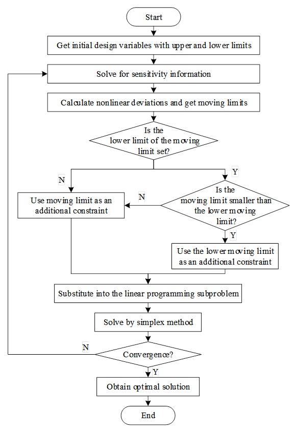
The size of the moving limit determines the accuracy of the linear programming model, which generally depends on the specific problem. In this paper, the moving limit is determined based on the nonlinear deviation of the objective and constraint functions, which is defined as: \[\label{GrindEQ__10_} d^{(k)} =\max \left(\left|\frac{f\left(x^{(k)} \right)-f^{(k-1)} \left(x^{(k)} \right)}{f\left(x^{(k)} \right)} \right|,\left|\frac{h_{i} \left(x^{(k)} \right)-h_{i}^{(k-1)} \left(x^{(k)} \right)}{h_{i} \left(x^{(k)} \right)} \right|\right) . \tag{8}\]
Then the moving limit of the \(k+1\)st iteration is: \[\label{GrindEQ__11_} s^{(k+1)} =\sqrt{\frac{\delta ^{(k+1)} }{d^{(k)} } } s^{(k)} , \tag{9}\] where \(\delta ^{(k+1)}\) is the nonlinear deviation to be controlled in the \(k+1\) round of iterations, usually selected empirically, the nonlinear deviation will affect the convergence speed, after testing this paper defaults to 0.6. The moving limit of the first round of iterations is taken as 10% of the corresponding design variables. The moving limit determined according to the formula (9) will decrease with the increase of the number of iterations, so as to improve the accuracy of the Taylor expansion and the performance of the sequential linear programming.
There are some limitations in the application of linear programming method for the design research process, such as the large amount of computation, constraints processing difficulties and other problems. Therefore, there is a need to explore an effective optimization algorithm to be used in the process of optimization and design of mechanical equipment structure.
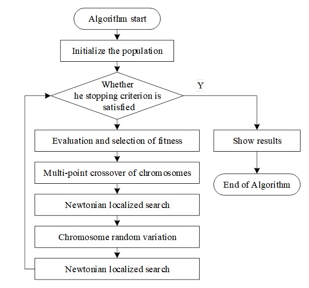
The cultural genetic algorithm (Memetic), in essence, is a combination of population-based global search and individual-based local heuristic search [1]. The Memetic algorithm process is very similar to GA, and the key difference is that the Memetic algorithm has an additional local search optimization process after crossover and mutation. For the function optimization problem, the traditional genetic algorithm is capable of global optimization, but it is prone to premature growth. For the traditional local search algorithm, it starts from an initial solution and searches for a better solution than it in its neighborhood, it can quickly find out the better solution, and its shortcoming is mainly that its faster local search performance can only be exerted when the initial value of iteration is in the vicinity of the real solution. The Memetic algorithm fully absorbs the advantages of both genetic algorithms and the traditional local search algorithms, and adopts the operation process of genetic algorithms, but after each crossover and mutation, the local search is carried out. However, local search is carried out after each crossover and mutation, and the undesirable population is eliminated early by optimizing the population distribution, which in turn reduces the number of iterations.
In this paper, the strategy of combining adaptive crossover, variation and proposed Newton local search is used to improve the execution strategy of Memetic algorithm to solve the transformed function optimization problem, and the specific Memetic algorithm operates as follows:
1) Coding: binary coding is used, and the length of the chromosome is determined according to the range of the value of the independent variable and the accuracy of the solution, which is generally between 20 and 50.
2) Fitness function: Because a nonlinear system may admit multiple solutions, the problem \(\min_{x\in D} g(x)\) can have multiple local/global optima. We therefore adopt a multi-evolution strategy. To discourage redundant searches across successive evolutions, the best solution from each evolution is stored in a global array \(X_a=\{X_a[1],\dots,X_a[L]\}\). Before the next evolution starts, any candidate \(x\) that falls within a \(\delta\)-neighborhood of a previously found solution is penalized, i.e., if \(x \in \bigcup_{k=1}^{L}\mathcal{O}(X_a[k],\delta)\) (with \(\mathcal{O}(X_a[k],\delta)=\{y:\|y-X_a[k]\|\le\delta\}\)), then its fitness is set to a large constant. Hybridization is then performed between the current best individual and randomly selected individuals. The fitness function is defined as \[\label{eq:fitness_penalty} f(x)= \begin{cases} C, & x \in \displaystyle\bigcup_{k=1}^{L}\mathcal{O}\!\left(X_a[k],\delta\right),\\[6pt] g(x), & \text{otherwise}, \end{cases} \tag{10}\] where \(C\gg 1\) is a large penalty constant and \(L\) is the number of (optimal) solutions found so far. Smaller values of \(f(x)\) indicate better individuals.
3) Crossover: We employ multi–point crossover. The crossover probability \(P_c\) controls how often the swapping operation is applied and is adapted according to population fitness: \[\label{eq:pc_adapt} P_c = \begin{cases} P_c \,\dfrac{f_{\max} – f_{\text{parent}}^{\max}}{f_{\max} – f_{\text{avg}}}, & f_{\text{parent}}^{\max} \ge f_{\text{avg}}, \\[8pt] P_c, & f_{\text{parent}}^{\max} < f_{\text{avg}}, \end{cases} \tag{11}\] where \(f_{\text{parent}}^{\max}\) is the larger fitness value of the two parents selected for crossover at the current step, \(f_{\max}\) is the best (maximum) fitness in the current population, and \(f_{\text{avg}}\) is the population’s average fitness.
4) Mutation: We use random–point mutation. The mutation probability \(P_m\) governs the fraction of new genes introduced into the population and is adapted as \[\label{eq:pm_adapt} P_m = \begin{cases} P_m \,\dfrac{f_{\max} – f(x)}{f_{\max} – f_{\text{avg}}}, & f(x) \ge f_{\text{avg}}, \\[8pt] P_m, & f(x) \le f_{\text{avg}}, \end{cases} \tag{12}\] where \(f(x)\) is the fitness of the individual undergoing mutation at the current step.
5) Local search strategy: To accelerate convergence on nonlinear systems and leverage the speed and accuracy of classical numerical methods, we embed a quasi-Newton (BFGS) local search within the Memetic framework. Offspring generated at each reproduction step are, with probability \(P_{n}\), refined by the following procedure.
Step 1. Iterate over the population and apply Steps 2–4 to each individual.
Step 2. For the \(i\)-th individual, draw \(r \sim \mathcal{U}(0,1)\).
Step 3. If \(r \le P_{n}\), perform two quasi-Newton line-search steps:
(3.1)First step. Let \(x^{(k)}\) be the current point, \(g_{1}=\nabla f\!\left(x^{(k)}\right)\), and set \(H_{1}=I\) (identity, sized to the decision space). Compute the descent direction \(d^{(1)}=-H_{1}g_{1}\) and perform a (one-dimensional) line search to obtain \[\lambda_{1}\;\in\;\arg\min_{\lambda \ge 0}\; \phi_{1}(\lambda) \;=\; f\!\bigl(x^{(k)}+\lambda\,d^{(1)}\bigr).\] Update \(x^{(k+1)} = x^{(k)} + \lambda_{1} d^{(1)}\).
(3.2)BFGS update and second step. Define \[p^{(1)} = x^{(k+1)} – x^{(k)} = \lambda_{1} d^{(1)},\qquad g_{2}=\nabla f\!\left(x^{(k+1)}\right),\qquad q^{(1)} = g_{2} – g_{1}.\] Set \(\rho_{1} = 1/\bigl(q^{(1)T}p^{(1)}\bigr)\) and update the inverse-Hessian approximation by the standard BFGS formula \[H_{2} = \bigl(I – \rho_{1} p^{(1)} q^{(1)T}\bigr)\,H_{1}\,\bigl(I – \rho_{1} q^{(1)} p^{(1)T}\bigr) + \rho_{1} p^{(1)} p^{(1)T}.\] Compute \(d^{(2)}=-H_{2}g_{2}\) and perform a line search \[\lambda_{2}\;\in\;\arg\min_{\lambda \ge 0}\; \phi_{2}(\lambda) \;=\; f\!\bigl(x^{(k+1)}+\lambda\,d^{(2)}\bigr),\] then set \(x^{(k+2)} = x^{(k+1)} + \lambda_{2} d^{(2)}\) as the refined offspring.
Step 4. The refined offspring \(x^{(k+2)}\) replaces its parent in the new population.
The study takes the optimal design analysis of main girder of bridge crane as an example, and uses the algebraic optimization method to carry out the optimal design of lightweight structure.
The main girder structure of an overhead crane, which is mainly responsible for and transfers the burden of the crane and its self-weight, is an important component of the whole structure of the crane. Most of the design optimization problems for the main girder of an overhead crane are highly nonlinear, including different design variables and complex stress, displacement, load carrying capacity and geometric configuration constraints. Therefore, the establishment of an accurate and reasonable mathematical model plays a very important role in solving the problem.
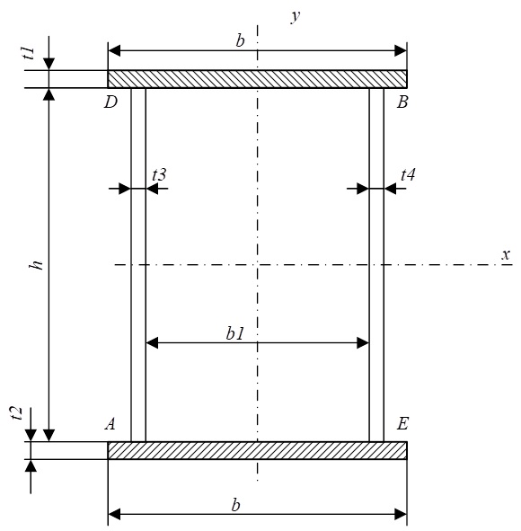
The main girder of a crane is usually a box section made of structural steel plates, consisting of main and sub webs, top and bottom flanges.The parameters of the main girder section are shown schematically in Figure 3. In general, they have different thicknesses. Since the optimization task is to obtain the minimum deadweight, i.e., minimum main girder cross-sectional area, while satisfying the given conditions. The variable parameters of the main beam are summarized in Table 1.
| Parameter name | Parameter symbol |
|---|---|
| Flange (mm) | b |
| Flange spacing (mm) | h |
| Main abdominal thickness (mm) | t3 |
| Secondary abdominal thickness (mm) | t4 |
| Upper flange thickness (mm) | t1 |
| Lower flange thickness (mm) | t2 |
The design variables are expressed as a column vector: \[\label{eq:design_vars} X = [\,b,\, t_1,\, t_2,\, h,\, t_3,\, t_4\,]^{T} = [\,x_1,\, x_2,\, x_3,\, x_4,\, x_5,\, x_6\,]^{T}. \tag{13}\]
Crane solid-web girders are typically welded box sections made of structural steel plates, comprising primary and secondary webs and upper and lower flanges. The optimization objective is to minimize self-weight—equivalently, the main girder’s cross-sectional area—while satisfying the design conditions for a given span. In this work, an off-track box-type main girder is considered, and the objective function is \[\label{GrindEQ__16_} \min_{x}\; f(x)\;=\;A(x)\;=\;x_{1}\bigl(x_{2}+x_{3}\bigr)\;+\;x_{4}\bigl(x_{5}+x_{6}\bigr), \tag{14}\] where \(A(x)\) denotes the cross-sectional area.
In order to make the design variables satisfy the structural strength, stiffness, stability, manufacturing process and dimensional constraints, the following constraints can be determined according to the Crane Design Manual.
The boundary constraints of the design variables need to consider that the upper and lower limit values of the design variables should not range too large, and a reasonable range should be selected, otherwise the search efficiency of the algorithm will be affected. According to querying the Crane Design Manual, the range of values of the six parameter vectors in the main girder section is determined as shown in Table 2.
| Variable | x1 | x2 | x3 | x4 | x5 | x6 |
|---|---|---|---|---|---|---|
| Max (mm) | 300 | 6 | 6 | 650 | 6 | 6 |
| Min (mm) | 700 | 32 | 32 | 1900 | 10 | 10 |
When the load acts at midspan, the maximum positive (tensile) stress occurs in the flanges at the section of maximum bending moment. The normal stress at the checked section must satisfy \[\label{GrindEQ__17_} \sigma \;=\; \frac{M_x}{W_x} \;+\; \frac{M_y}{W_y} \;\le\; [\sigma], \tag{15}\] where \(M_x\) is the bending moment due to vertical loading on the main girder section (N\(\cdot\)mm), \(M_y\) is the bending moment in the checked section due to horizontal inertia when the trolley starts/brakes (N\(\cdot\)mm), and \(W_x\), \(W_y\) are the section moduli in the vertical and horizontal directions, respectively. The allowable stress is \[\label{GrindEQ__18_} [\sigma] \;=\; \frac{\sigma_s}{n_s}, \tag{16}\] with \(\sigma_s\) the steel yield strength and \(n_s\) the safety factor.
Considering the locations \(A\) and \(B\) (Figure 3) where the free-bending normal stress attains its maximum, the constraints are \[\label{GrindEQ__19_} g_1(x) \;=\; \frac{\sigma_A}{[\sigma]} – 1 \;\le\; 0, \qquad g_2(x) \;=\; \frac{\sigma_B}{[\sigma]} – 1 \;\le\; 0, \tag{17}\] where \(\sigma_A\) and \(\sigma_B\) are the peak normal stresses at points \(A\) and \(B\) of the critical midspan section.
The web at the span end carries the largest shear and is used for checking. The shear stress must satisfy \[\label{GrindEQ__21_} \tau \;=\; \frac{Q_{\max}\, S_x}{I_x\, \delta_3} \;+\; \frac{M_n}{2 A_0\, \delta_3} \;\le\; [\tau], \tag{18}\] where \(I_x\) is the second moment of area of the checked section (mm\(^4\)), \(S_x\) is the first moment of area about the neutral axis for the portion of the section carrying shear (N\(\cdot\)mm), \(\delta_3\) is the web thickness (mm), and \(A_0\) is the area of the checked section (mm\(^2\)). The maximum shear force is \[\label{GrindEQ__22_} Q_{\max} \;=\; Q_b \;+\; Q_q, \tag{19}\] where \(Q_b\) is due to the self-weight of the main girder (N), and \(Q_q\) is due to the trolley wheel loads (N). The torsional (warping) term is \[\label{GrindEQ__23_} M_n \;=\; M_{pns} \;+\; M_{bns} \;+\; M_{pmc}, \tag{20}\] where \(M_{pns}\) is the torque from horizontal inertia of moving loads (N\(\cdot\)mm), \(M_{bns}\) is the torque from the girder’s self-weight (N\(\cdot\)mm), and \(M_{pmc}\) is the torque from eccentric trolley wheel loads (N\(\cdot\)mm). The corresponding constraint is \[\label{GrindEQ__24_} g_3(x) \;=\; \frac{\tau}{[\tau]} – 1 \;\le\; 0. \tag{21}\]
At the dangerous welds \(D\) and \(E\) in the midspan region, the fatigue constraints are \[\label{GrindEQ__25_} g_4(x) \;=\; \frac{1}{1.1}\!\left[ \left(\frac{\sigma_{D x,\max}}{[\sigma_{x r}]}\right)^{\!2} +\left(\frac{\sigma_{m}}{[\sigma_{y r}]}\right)^{\!2} -\frac{\sigma_{D x,\max}\,\sigma_{m}}{[\sigma_{x r}]\,[\sigma_{y r}]} +\left(\frac{\tau_{D}}{[\tau_{x p r}]}\right)^{\!2} \right] – 1 \;\le\; 0, \tag{22}\] \[\label{GrindEQ__26_} g_5(x) \;=\; \frac{1}{1.1}\!\left[ \left(\frac{\sigma_{E x,\max}}{[\sigma_{x r}]}\right)^{\!2} +\left(\frac{\tau_{E}}{[\tau_{x y r}]}\right)^{\!2} \right] – 1 \;\le\; 0, \tag{23}\] where \([\sigma_{x r}]\) is the allowable tensile/compressive fatigue stress corresponding to \(\sigma_{D x,\max}\) (or \(\sigma_{E x,\max}\)), \([\sigma_{y r}]\) is the allowable compressive fatigue stress corresponding to the mean stress \(\sigma_m\), and \([\tau_{x p r}]\), \([\tau_{x y r}]\) are the allowable shear fatigue stresses corresponding to \(\tau_D\) and \(\tau_E\), respectively. Here, \(\sigma_{D x,\max}\) and \(\sigma_{E x,\max}\) are the maximum normal stresses at \(D\) and \(E\), and \(\tau_D\), \(\tau_E\) are the corresponding maximum shear stresses.
Under service loads, the main beam’s static stiffness is characterized by its deflection; the maximum midspan deflection must not exceed the permissible limit. In practice, ancillary components (platforms, railings, etc.) also contribute to overall stiffness.
The horizontal static deflection is evaluated as \[\label{GrindEQ__27_} f_{H} =\frac{(P_{1}+P_{2})L^{3}}{48EI_{y}}\!\left(1-\frac{3L}{4r}\right) +\frac{5q_{L}L^{4}}{384EI_{y}}\!\left(5-\frac{4L}{r}\right) \;\le\;[f_{H}], \tag{24}\] where \(P_{1}\) is the wheel load due to the lifted mass (N), \(P_{2}\) is the wheel load due to the trolley self-weight (N), \(q_{L}\) is the inertia force from the girder self-weight (N), \(E\) is the elastic modulus (Pa), \(L\) is the span (mm), \(B\) is the trolley wheelbase (mm), and \([f_{H}]\) is the allowable horizontal static deflection. The parameter \(r\) is given by \[r \;=\; L \;+\; \frac{8C^{3}+l^{3}}{3B^{2}}\cdot\frac{I_{1}}{I_{2}},\qquad C=\frac{B-l}{2}.\]
The vertical static deflection is computed as \[\label{GrindEQ__28_} f_{V} =\frac{(P_{1}+P_{2})\Bigl(0.75L^{2}-\bigl(\tfrac{L-b}{2}\bigr)^{2}\Bigr)\bigl(\tfrac{L-b}{2}\bigr)} {12EI_{x}} \;\le\;[f_{V}], \tag{25}\] where \(b\) is the trolley wheelbase (mm) and \([f_{V}]\) is the allowable vertical static deflection.
Thus, the static stiffness constraints are \[\label{GrindEQ__29_} g_{6}(x)=\frac{f_{H}}{[f_{H}]}-1\;\le\;0,\qquad g_{7}(x)=\frac{f_{V}}{[f_{V}]}-1\;\le\;0, \tag{26}\] where \(f_{H}\) and \(f_{V}\) are the maximum horizontal and vertical midspan deflections, respectively, and \([f_{H}]\), \([f_{V}]\) are the corresponding allowable limits. For duty class A5, \([f_{H}]=L/2000\) and \([f_{V}]=L/800\).
With the trolley fully loaded and positioned in the span, the main beam exhibits vertical and horizontal natural vibrations. The corresponding fundamental frequencies must meet prescribed limits. A common vertical check is \[\label{GrindEQ__31_} f_{v} \;=\; \frac{1}{2\pi}\sqrt{\frac{g}{\bigl(y_{0}+\lambda_{0}\bigr)\,(1+\beta)}} \;\ge\; [f_{v}], \tag{27}\] and the frequency constraints can be written as \[\label{GrindEQ__32_} g_{8}(x)=[f_{h}]-f_{h}\;\le\;0,\qquad g_{9}(x)=[f_{v}]-f_{v}\;\le\;0, \tag{28}\] where \([f_{v}]\) and \([f_{h}]\) are the allowable vertical and horizontal natural frequencies, typically \([f_{v}]\in[2,4]\ \mathrm{Hz}\) and \([f_{h}]\in[1.5,2]\ \mathrm{Hz}\).
The height-to-span ratio of the main beam is typically chosen in the range \[\label{GrindEQ__34_} \frac{h}{L} \;\in\; \left[\frac{1}{18},\,\frac{1}{14}\right], \tag{29}\] taking the larger value for shorter spans and the smaller value for longer spans.
As shown in Figure 3, the combined (equivalent) stress at point \(D\) (connection of the main web and the upper flange) is constrained by \[\label{GrindEQ__35_} \sigma_{c,D} \;=\; \sqrt{\sigma_{D x,\max}^{2} + \sigma_{m}^{2} – \sigma_{D x,\max}\,\sigma_{m} + 3\,\tau_{D}^{2}}, \tag{30}\] where \(\sigma_{D x,\max}\) is the maximum normal (positive) stress at \(D\), \(\sigma_{m}\) is the contact (bearing) stress at \(D\) due to wheel load, and \(\tau_{D}\) is the shear stress at \(D\). The corresponding constraint is \[\label{GrindEQ__36_} g_{10}(x) \;=\; \frac{\sigma_{c,D}}{[\sigma]} – 1 \;\le\; 0, \tag{31}\] with \([\sigma]\) the allowable equivalent stress.
The minimum clear spacing between the two webs of the main beam satisfies \[\label{GrindEQ__37_} b_{0} \;=\; b – c \;\ge\; 300, \qquad c \in [40,\,60], \tag{32}\] where \(b\) is the web-to-web distance (overall), \(c\) is the allowance for local details (e.g., fillets/stiffeners), and \(b_{0}\) is the resulting clear spacing (all dimensions in mm).
After the model design and topology optimization of the new structure of the parts in the early stage, it is not yet possible to carry out direct additive manufacturing processing, and the newly designed parts also need to use finite element tools to carry out static mechanical performance verification, modal analysis and other simulation experiments to verify the reliability of the innovative structure.
The geometrical structure of the topological space is studied by transforming it into a group based on homotopy groups and setting the parameter values of the main beam structure using the Memetic algorithm proposed above.
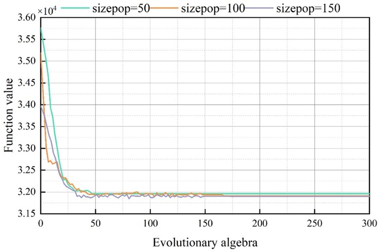
The size of the population size is selected according to the difficulty of solving the problem, such as the number of peaks of the solution function and the number of constraints. In general, the larger the population size, the better the population diversity, the stronger the global search ability, and at the same time, its search accuracy will be correspondingly improved, and the faster the convergence speed will be, but the larger the population size, the larger the computational volume, and the longer the time of its solving computation will be. All other parameters in the algorithm are set the same, and the population size of 50, 100, 150 were selected for calculation and testing for 30 times. The relevant data obtained during the calculation process are shown in Table 3, and in order to visualize the performance of the algorithm parameters, the floating-point type data comparison is used directly. The curve graph of the results of one test is randomly selected for comparison, and its optimal individual fitness change curve is shown in Figure 4. Combined with Table 3 and Figure 4 for analysis, in the case of other settings of the algorithm are the same, it is found that when the population size is 50, its iterative computation converges prematurely, and it is easy to fall into the local optimum, and the global search ability is poor. Under a limited number of iterations, its converged optimal solution is worse than the solutions obtained when the population size is 100 and 150. The optimal fitness change curves are similar when the population size is 100 and 150 respectively, and the solutions obtained at the end are basically the same, and the values of their design variables are basically the same after rounding. In addition, the average number of optimal solution generations for population size 100 is 166, and the average number of optimal solution generations for population size 150 is 177, compared to which the algorithm for population size 100 has a faster convergence speed on average, and the amount of computation is relatively small. Through the above comparisons, the population size sizepop=100 is selected after comprehensively considering the factors such as the advantages and disadvantages of the solutions, the convergence speed, and the size of the computation.
| Parameter Project | x1 | x2 | x3 | x4 | x5 | x6 | f(x) | Optimal algebra |
|
Population quantity
N=50 |
696.44 | 9.97 | 9.98 | 1491.62 | 6 | 6.02 | 31907.12 | 191 |
| 696.24 | 9.92 | 9.91 | 1493.47 | 6.03 | 6.04 | 31888.24 | 187 | |
| 694.24 | 9.97 | 10 | 1502.35 | 6.02 | 6.04 | 31877.67 | 150 | |
| 694.74 | 9.99 | 9.97 | 1500.02 | 6.05 | 6.05 | 31904.48 | 134 | |
| 697.94 | 9.95 | 9.94 | 1498.09 | 6.05 | 6.04 | 31877.99 | 171 | |
| Mean | 695.42/9.96/9.97/1496.87/6.03/6.04 | 31894.38 | 136 | |||||
|
Population quantity
N=100 |
695.11 | 9.99 | 9.92 | 1498.61 | 6.04 | 6 | 31895.23 | 198 |
| 694.21 | 9.96 | 9.97 | 1492.06 | 6.03 | 6.01 | 31879.82 | 145 | |
| 695.65 | 9.96 | 9.95 | 1494.25 | 6.05 | 6.01 | 31876.18 | 186 | |
| 694.55 | 9.93 | 9.96 | 1499.05 | 6.01 | 6.02 | 31860.97 | 140 | |
| 695.43 | 9.95 | 9.93 | 1496.17 | 6.02 | 6.01 | 31864.1 | 194 | |
| Mean | 696.33/9.95/9.94/1497.99/6.02/6.03 | 31924.14 | 166 | |||||
|
Population quantity
N=150 |
696.17 | 9.95 | 9.93 | 1495.52 | 6.01 | 6 | 31869.24 | 133 |
| 695.45 | 9.96 | 9.96 | 1490.07 | 6.04 | 6.02 | 31866.63 | 190 | |
| 694.45 | 9.97 | 9.97 | 1493.5 | 6.05 | 6.04 | 31889.63 | 153 | |
| 696.45 | 9.97 | 9.95 | 1491.22 | 6.06 | 6.01 | 31918.3 | 176 | |
| 695.42 | 9.98 | 9.96 | 1496.09 | 6.03 | 6.06 | 31895.65 | 196 | |
| Mean | 696.27/9.93/9.91/1496.93/6.01/6 | 31914.32 | 177 | |||||
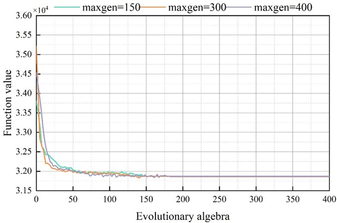
In the process of optimization calculation, the solution result will gradually converge with the increase of iteration number, and finally satisfy the termination condition, so the choice of the maximum number of times directly determines the advantages and disadvantages of the optimization result. If the number of iterations is too small, the early termination of the calculation may occur, and the number of iterations is too large, which may cause a waste of computing resources. Therefore, in this paper, in the case of population size of 100, the maximum number of iterations are selected as 150, 300 and 400 for the test, and the data obtained are analyzed by statistical comparison. Each case is tested 30 times, and the statistical comparison data are shown in Table 4, and the change curve of the optimal individual fitness at different maximum iteration times is shown in Figure 5. Combined with Figure 5 and Table 4, it can be analyzed that, when the population size is 100, and under the premise of other parameter settings are also the same, it can be obtained from Figure 5 that, when the maximum number of iterations is 150, the evolutionary iteration stops at the 144th generation, and the obtained optimal solution is poorer than that obtained at the maximum number of iterations of 300 and 400, respectively, the iteration is terminated too early, and the iterative computation has not yet converged to the optimal solution. As can be seen from Table 4, the two cases when the number of iterations is 300 and 400 respectively, the objective function values obtained from the optimization are very close, and the average number of optimal solution generations of the former appeared around the 176th generation, compared with the latter, convergence is good, and the amount of computation is also relatively small. The maximum number of iterations maxgen=300 is selected after considering the quality of the solution, the convergence of the algorithm and the amount of computation.
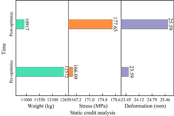
In order to deeply investigate whether the optimized main girder structure meets the strength and stiffness requirements of the crane, the optimized main girder structure model is subjected to static analysis. The comparison of the static analysis results before and after optimization is shown in Figure 6. The mass of the main girder before and after optimization is 12,572kg and 10,917kg respectively, which is reduced by 1,655kg, with an optimization rate of 13%, and the quality target optimization effect is remarkable. According to the “Crane Design Code” (GB/T 3811-2008) about the maximum static deflection of the main girder of the bridge crane \(\mathrm{\le}\) S/1000, the permissible static deflection should be less than 32mm, and the permissible stress should be less than 181Mpa.The maximum stress of the optimized main girder structure is 177.65Mpa, and the maximum deflection deformation of the span is 25.595mm, and the strength, stiffness calibration is passed. The optimized main girder structure meets the design requirements. Therefore, the main girder structure of the crane has better static characteristics and deformation resistance after optimization.
| Parameter Project | x1 | x2 | x3 | x4 | x5 | x6 | f(x) | Optimal algebra |
|
Cut-off algebra
Kmax=150 |
695.06 | 10 | 9.91 | 1495.61 | 6.02 | 6.03 | 31864.51 | 176 |
| 695.17 | 9.92 | 9.92 | 1501.91 | 6.03 | 6.03 | 31886.58 | 130 | |
| 697.18 | 9.99 | 9.98 | 1492.62 | 6.03 | 6.01 | 31916.42 | 146 | |
| 695.71 | 9.93 | 9.98 | 1490.49 | 6.03 | 6.04 | 31883.4 | 195 | |
| 696.52 | 9.95 | 9.97 | 1493.6 | 6.05 | 6.01 | 31907.34 | 196 | |
| Mean | 695.27/9.97/9.91/1486.53/6.01/6.01 | 31905.14 | 95 | |||||
|
Cut-off algebra
Kmax=300 |
695.78 | 9.97 | 9.92 | 1502.12 | 6.03 | 6.02 | 31904.91 | 152 |
| 697.71 | 9.91 | 9.98 | 1500.04 | 6.03 | 6.05 | 31919.87 | 180 | |
| 697.9 | 9.99 | 9.91 | 1498.18 | 6.02 | 6.06 | 31905.1 | 156 | |
| 694.68 | 9.91 | 9.93 | 1497.31 | 6.03 | 6.05 | 31891 | 149 | |
| 695.7 | 9.96 | 9.99 | 1493.38 | 6.02 | 6.02 | 31860.74 | 176 | |
| Mean | 696.33/9.94/9.95/1473.51/6/6.02 | 31963.22 | 176 | |||||
|
Cut-off algebra
Kmax=400 |
696.13 | 9.93 | 9.91 | 1501.15 | 6.02 | 6.06 | 31862.78 | 145 |
| 695.48 | 9.96 | 9.91 | 1501.13 | 6.02 | 6.02 | 31903.72 | 150 | |
| 697.04 | 9.98 | 9.92 | 1494.69 | 6.03 | 6.03 | 31905.61 | 189 | |
| 695.73 | 9.98 | 9.91 | 1499.8 | 6.02 | 6.04 | 31865.73 | 193 | |
| 695.59 | 9.92 | 9.93 | 1496.09 | 6.05 | 6.04 | 31917.96 | 152 | |
| Mean | 696.37/9.94/9.93/1487.44/6.03/6.02 | 31955.24 | 185 | |||||
Modal analysis, i.e., free vibration analysis, can be used to derive the intrinsic frequency and vibration pattern of a structure, thus enabling the structure to avoid resonance and predicting the form of vibration of the structure under different loads. In addition, modal analysis can also determine the self-oscillation period of the structure, thus helping analysts to determine a reasonable transient analysis time step.
Bridge cranes are usually accompanied by starting and braking along the track and frequent lifting and lowering of goods by the trolley pickup device in the working process, and these motions usually bring a certain amount of shock vibration to the whole machine, which will generate a lot of noise and reduce the service life of the whole machine in serious cases, and thus it is necessary to carry out a modal analysis of the crane.
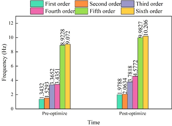
Before and after the optimization of the main girder structure of each order frequency comparison shown in Figure 7. Before optimization, the inherent frequency of the vertical direction of the bridge is 3.3652Hz, and after optimization, the inherent frequency of the vertical direction of the bridge is increased to 3.7818Hz, with an optimization rate of 12.38%. The dynamic performance target optimization effect is remarkable.
This subsection analyzes the transient dynamics of the main girder structure of an overhead crane with the aim of investigating the dynamic excitation of the main girder during the lifting process of the article. During the lifting process of the article, when the article is suddenly off the ground, the inertia caused by the lifting of the article will bring shock vibration to the main girder. In order to verify the dynamic performance of the main girder in the most unfavorable lifting position, the lifting process when the trolley is located at the end is selected for the study. Crane trolley for item lifting can be divided into the following three stages.
1) The hook of the fetching device hangs up the goods and starts to lift, at this time, the wire rope on the pulley block is in a state of relaxation, and when the lifting height gradually increases, the wire rope starts to be tightened.
2) With the tightening phase of the wire rope, the force on the wire rope can be approximated as a linear change phase. The excitation load brought by lifting the goods will make the main beam start to vibrate, in this process, the goods have been located on the ground, until the internal force of the wire rope is close to and equal to the gravity of the goods.
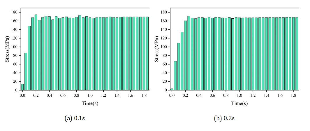
3) The goods leave the ground, at this time the goods are lifted more smoothly, the force of the wire rope remains constant, equal to the gravity of the lifted items. In the first stage of the crane trolley for goods lifting, the wire rope is not stressed, the main analysis is the wire rope starts to tension until the goods leave the ground smoothly stage, to verify the safety performance of the main beam under the changing load. For the selection of the main beam time step, divided into two stages, the first stage is from the wire rope pulling up to the tensioning stage, the second stage is the rapid rise of the goods stage, for the first stage of the faster time, respectively, take 0.1s and 0.2s as the end time, after a number of tests, the end of the second stage of the time is set at 2 s. The damping ratio of the metal structure of the crane is generally 0.008-0.05. The stress response of the main beam structure is 0.008-0.05. The main analysis is that the wire rope is not under tension until the goods leave the ground smoothly.
The stress response of the main girder structure is shown in Figure 8, (a) and (b) indicate that the end time is 0.1s and 0.2s, respectively (the same below). From the figure, it can be seen that in the initial stage of lifting the goods, the main beam stress appeared in the vertical direction of the step-like elevation, and the maximum stress of the main beam in the off-ground time of 0.1s and 0.2s reaches 174.63MPa and 170.82MPa, respectively.It indicates that the shorter the loading time of the wire rope is, the greater the maximum stress appeared on the main beam, and the excitation of the crane is more obvious. In practice, slowing down the lifting process of the cargo is of great significance to the maintenance of the crane. With the effect of damping, the amplitude began to decrease, located after 1.08s, the stress of both structures tend to stabilize state.
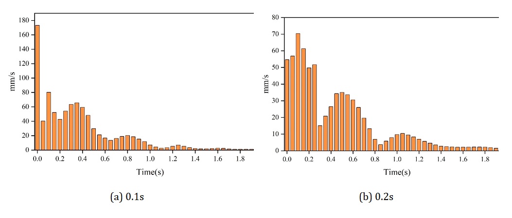
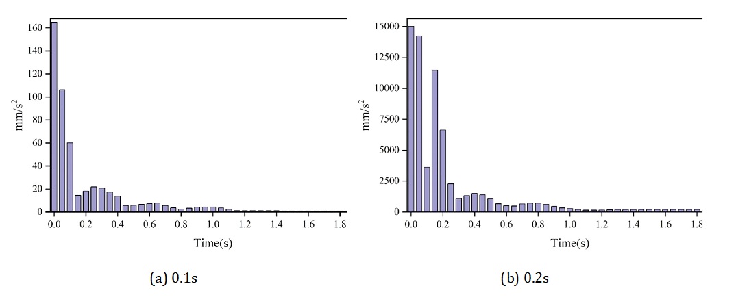
The velocity response of the main beam structure is shown in Figure 9. The acceleration response of the main beam structure is shown in Figure 10. From the velocity and acceleration graphs, it can be seen that the shorter the time given to the wire rope tightening phase, the greater the amplitude of the velocity and acceleration, which will cause a greater impact on the main beam, so when setting the time for the crane to lift the goods, it should be as long as possible to make the time away from the ground, so that the goods can be lifted smoothly.
Summarize. The maximum deflection of the optimized main girder structure was increased by 8% compared to the original structure, and the maximum equivalent stress and mass were reduced by 7% and 13%, respectively. After that, the main girder was analyzed based on reliability, modal and transient dynamics respectively, and the results showed that the optimized main girder was safer in these aspects.
The study combines algebraic topological methods for lightweight structural optimization design of automated mechanical equipment, taking the main girder structure of an overhead crane as an example, and using mathematical formulas to describe the actual structural optimization problem of this project. According to the Crane Design Manual, it is determined that the optimization design problem of the bridge crane is a multi-constraint, multi-variable non-linear constrained optimization problem, so the Memetic algorithm is used for parameter solving. The population size and the maximum number of evolutionary iterations of the main girder structure are finally solved to be 100 and 300, respectively, and the reasonableness of the design of the main girder structure is verified in terms of statics and dynamics. The maximum deformation of the optimized main girder is 8% higher than that of the original structure, and the maximum stress and mass are reduced by 7% and 13%, respectively. Modal and transient dynamics analysis of the structure is carried out, and the optimization effect of the dynamic performance target is remarkable. The methodology of this paper provides a feasible solution for lightweight design.