
Vertex coloring is perhaps the most popular topic in graph theory.
Definition 1.1. A proper vertex coloring of a graph is a function \(c:V\left(G\right)\rightarrow\left\{ 1,\ldots,k\right\}\) that assigns one color to each vertex so that that adjacent vertices are colored differently. A \(k\)-coloring of a graph is a proper vertex coloring using colors \(\left\{ 1,\ldots,k\right\}\) (not necessarily all of them). A graph is \(k\)-colorable if it has a \(k\)-coloring. The chromatic number \(\chi\left(G\right)\) is the minimum number of colors used in any \(k\)-coloring of a graph \(G\). A graph with \(\chi\left(G\right)=k\) is said to be \(k\)-chromatic. An optimal coloring of a graph is one using \(\chi\left(G\right)\) colors.
Determining the chromatic number when it is larger than two is an NP-complete problem, meaning that it is difficult to efficiently determine in general. Because of this, a major issue in chromatic graph theory is to determine upper and lower bounds for the chromatic number in terms of graph parameters that can be calculated efficiently. If the bounds are good, they may be equal for a graph in question, solving the problem in that case.
One simple way to color the vertices of a graph is to color them one at a time using some ordering of the vertices. The greedy coloring algorithm assigns each vertex the least color that has not already been used on any of its neighbors that are already colored.
It is well-known that for any graph \(G\), there is some vertex ordering so that applying greedy coloring will result in an optimal coloring. Indeed, given a coloring \(c\left(v\right)\) with \(\chi\left(G\right)\) colors, such an ordering can be constructed by starting with all vertices colored 1, then all colored 2, etc. Of course, the problem is that finding this ordering requires already having an optimal coloring.
One could search all possible vertex orderings, but since there are \(n!\) possible orderings on \(n\) vertices, this is impractical for large graphs. Thus it is desirable to consider a smaller set of vertex orderings that are likely to attain, or at least come close to the minimum number of colors. Many different orderings have been considered [4]. The ordering that we will consider in this paper is SL ordering.
Definition 1.2. A deletion sequence of a graph \(G\) is an ordering \(v_{1},\dots,v_{n}\) of \(V\left(G\right)\) such that each \(v_{i}\) has minimum degree in the induced subgraph \(G[\{v_{i},v_{i+1},\dots,v_{n}\}]\). A smallest-last ordering (SL-ordering) of a graph is the reversal of a corresponding deletion sequence. A graph is \(k\)-degenerate if its vertices can be successively deleted so that when deleted, each has degree at most \(k\). The degeneracy \(D\left(G\right)\) of a graph \(G\) is the smallest \(k\) such that it is \(k\)-degenerate. The SL algorithm applies greedy coloring to an SL ordering of a graph.
The SL algorithm will produce a (not necessarily optimal) proper vertex coloring of the graph. It immediately implies the bound \(\chi\left(G\right)\leq1+D\left(G\right)\). This is superior to many common bounds on the chromatic number [2]. However, this can still be a poor bound when the degeneracy is much larger than the chromatic number, such as for complete multipartite graphs. Note however that the SL algorithm may not require \(1+D\left(G\right)\) colors.
Definition 1.3. A graph \(G\) is slightly hard-to-color (SHC) with respect to an algorithm if for some instance of it the number of colors used is more than \(\chi\left(G\right)\). A hard-to-color (HC) graph is one for which every application of the algorithm uses more than \(\chi\left(G\right)\) colors. An easy-to-color (EC) graph is one for which every application of the algorithm uses \(\chi\left(G\right)\) colors.
Kubale et al. [5] point out various classes of graphs that are EC for the SL algorithm. Notably, these include complete bipartite graphs (which easily generalize to complete multipartite graphs) and \(k\)-trees. (A \(k\)-tree is a graph that can be formed by starting with \(K_{k+1}\) and iterating the operation of adding a degree \(k\) vertex adjacent to all the vertices of a \(k\)-clique of the existing graph.)
Definitions of terms and notation not defined here appear in [2]. In particular, \(n\left(G\right)\) is the number of vertices of \(G\). When the context is clear, we use \(n\) to indicate the order of a graph. Given graphs \(G\) and \(H\), the join is \(G+H\), the cartesian product is \(G\square H\), and the square of \(G\) is \(G^{2}\). A dominating vertex of a graph is a vertex adjacent to all other vertices.
Both SHC and HC graphs exist for the SL algorithm. Kubale et al. [5] proved that \(K_{3}\square K_{2}\) is the smallest SHC graph for the SL algorithm. (This was later also proved in [1].)
In the following theorem, we discuss the probability that an SL ordering produces an optimal coloring for \(C_{2r+1}\square K_{2}\). The assumption we are making is that each valid choice for which vertex to delete in a deletion sequence is equally likely. This is not necessarily the same as treating all deletion sequences as equally likely.
Theorem 2.1. Each graph \(C_{2r+1}\square K_{2}\), \(r\geq1\), is SHC for the SL algorithm. The SL algorithm produces an optimal coloring (a 3-coloring) of \(C_{2r+1}\square K_{2}\) at most \(\frac{4}{9}\) of the time.
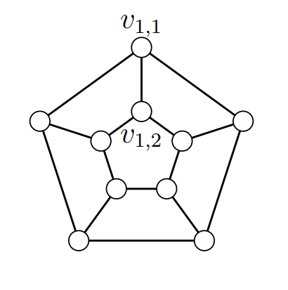
Proof. Denote the vertices of \(C_{2r+1}\square K_{2}\) as \(v_{i,j}\), \(1\leq i\leq2r+1\), \(1\leq j\leq2\), and let the two copies of \(C_{2r+1}\) be denoted by \(C\) and \(C'\) (see \(C_{5}\square K_{2}\) above). Since \(C_{2r+1}\square K_{2}\) is vertex-transitive, any vertex can be the first deleted in a deletion sequence. Thus we assume that an SL ordering for \(G\) ends with \(v_{1,1}\).
There is a \(\frac{1}{3}\) chance that \(v_{1,2}\) is deleted immediately after \(v_{1,1}\). Now \(C_{2r+1}\square K_{2}-\left\{ v_{1,1},v_{1,2}\right\} =P_{2r}\square K_{2}\), which is bipartite. No deletion sequence will disconnect \(P_{2r}\square K_{2}\), so the SL algorithm will 2-color it. Then the SL algorithm requires 4 colors for \(C_{2r+1}\square K_{2}\) in this case.
There is a \(\frac{2}{3}\) chance that another vertex (say \(v_{2,1}\)) is deleted immediately after \(v_{1,1}\). As in the previous case, it should be clear that if \(v_{1,2}\) is the first vertex in \(C'\) deleted, the SL algorithm will require 4 colors.
If \(2r+1=3\), then \(v_{3,1}\) must be deleted third. There is a \(\frac{1}{3}\) chance that \(v_{1,2}\) is deleted first in \(C'\). The other SL orderings produce a 3-coloring. Thus \(\frac{1}{3}+\frac{2}{3}\frac{1}{3}=\frac{5}{9}\) of the SL orderings require 4 colors.
Suppose \(2r+1\geq5\). Then there is a \(\frac{1}{4}\) chance that \(v_{1,2}\) is deleted third, and a \(\frac{2}{4}\) chance that \(v_{3,1}\) or \(v_{2r+1,1}\) was deleted third. As in the previous case, we see that at least \(\frac{1}{3}+\frac{2}{3}\left(\frac{1}{4}+\frac{2}{4}\frac{1}{5}\right)=\frac{17}{30}>\frac{5}{9}\) of the SL orderings require 4 colors. ◻
For a given value of \(2r+1\), the exact probability can be calculated if desired. When \(2r+1=5\), we find \(\frac{1}{3}+\frac{2}{3}\left(\frac{1}{4}+\frac{2}{4}\left(\frac{1}{5}+\frac{2}{5}\frac{1}{5}\right)\right)=\frac{89}{150}\approx.593\) of the SL orderings require 4 colors.
Kubale et al. [5] also proved that \(C_{8}^{2}\) (which they called the prismatoid) is the unique smallest HC graph for the SL algorithm. (Unaware of this result, I later wrongly conjectured in [1] that HC graphs for the SL algorithm did not exist.)
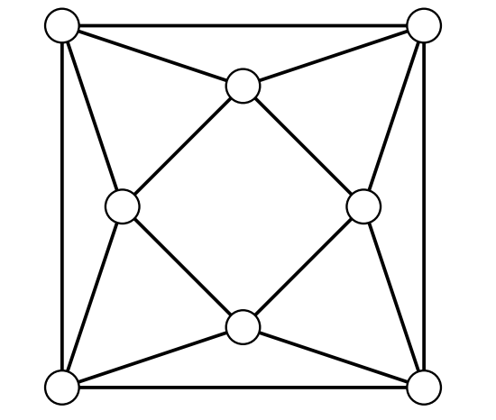
Theorem 3.1. (Kubale et al. [5]) The unique smallest HC graph for the SL algorithm is \(C_{8}^{2}\).
Note that \(\chi\left(C_{8}^{2}\right)=4\). Thus it is natural to ask for which other values of \(\chi\left(G\right)\) HC graphs exist for the SL algorithm. No bipartite graph is HC for the SL algorithm [5]. However, some bipartite graphs are SHC. This can occur when a minimum degree vertex is a cut-vertex of a bipartite graph.
Hansen and Kuplinsky [5] found a 3-chromatic HC graph for the SL algorithm with 33 vertices. Their example decomposes into three copies of \(K_{5,5}\) and one copy of \(Tr_{2}\) (the triangular grid with degree sequence 444222). Next I present an example with 10 vertices.
Let \(G_{10}\) have vertices \(A\cup B\cup C\), \(A=\left\{ a_{1},a_{2},a_{3}\right\}\), \(B=\left\{ b_{1},b_{2},b_{3},b_{4}\right\}\), \(C=\left\{ c_{1},c_{2},c_{3}\right\}\). Let \(A\cup B\) induce \(K_{3,4}\), \(C\) induce \(K_{3}\), and add edges \(\left\{ b_{1}c_{1},b_{2}c_{2},b_{3}c_{3},b_{4}c_{3}\right\}\) (see below).
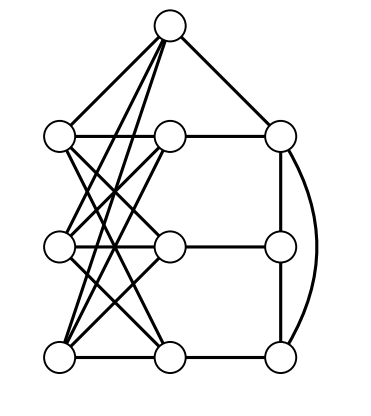
Theorem 3.2. The graph \(G_{10}\) is a HC graph for the SL algorithm.
Proof. Deleting vertices of minimum degree, we start with \(c_{1}\) and \(c_{2}\) (in either order), then \(c_{3}\), then some vertex of \(B\), then the rest of \(A\cup B\) in some order. Thus any SL ordering begins with \(A\cup B\) in some order, then \(c_{3}\), then \(c_{1}\) and \(c_{2}\) (in either order).
Applying greedy coloring to any SL ordering colors \(K_{3,4}\) uniquely (aside from permutation of colors). If \(A\) gets 1, \(B\) gets 2. Then \(c_{3}\) gets 1, and \(c_{1}\) and \(c_{2}\) get 3 and 4. If \(A\) gets 2, \(B\) gets 1. Then \(c_{3}\) gets 2, and \(c_{1}\) and \(c_{2}\) get 3 and 4. Thus any SL ordering requires 4 colors.
However, \(G\) has a 3-coloring, with 1 on \(\left\{ a_{1},a_{2},a_{3},c_{1}\right\}\), 2 on \(\left\{ b_{3},b_{4},c_{2}\right\}\), and 3 on \(\left\{ b_{1},b_{2},c_{3}\right\}\). Thus \(G\) has no SL ordering so that greedy coloring yields an optimal coloring. ◻
Kubale et al. [5] showed that there is no 3-chromatic HC graph for the SL algorithm with order less than 8, and none of order 8 with at most 16 edges. This required extensive case-checking, so it may not be feasible to determine whether \(G_{10}\) is the smallest such graph without a computer search.
Since Kubale et al. [5] showed that the unique smallest HC graph for the SL algorithm is \(C_{8}^{2}\), it may be interesting to know if other squares of cycles are HC. We generalize the argument they used for \(C_{8}^{2}\).
Theorem 3.3. For all \(r\geq2\), \(C_{3r+2}^{2}\), is a HC graph for the SL algorithm, while \(C_{3r}^{2}\) and \(C_{3r+1}^{2}\) <mindya'Pr j li
Proof.Let the vertices of \(C_{3r+t}\), \(0\leq t\leq2\), be \(v_{1}v_{2}\ldots v_{3r+t}v_{1}\). Since \(C_{3r+t}^{2}\) is vertex-transitive, we may assume \(v_{1}\) is the last vertex in an SL ordering. By symmetry, the next-to-last vertex is either \(v_{2}\) or \(v_{3}\). After the final two or three vertices, the problem is reduced to coloring a 2-tree, which has a unique 3-coloring (up to permutation of colors). We consider three cases, in each denoting the coloring of \(C_{3r+t}^{2}\) by \(c\left(v\right)\).
Let \(t=2\). Suppose the next-to-last vertex is \(v_{2}\). Then \(C_{3r+2}^{2}-v_{1}-v_{2}=P_{3r}^{2}\), which is a 2-tree. Any SL ordering will result in a unique 3-coloring of \(P_{3r}^{2}\). We see \(\left\{ v_{3}\right\}\), \(\left\{ v_{4},v_{3r+1}\right\}\), and \(\left\{ v_{3r+2}\right\}\) receive distinct colors from \(\left\{ 1,2,3\right\}\). Then \(c\left(v_{2}\right)=4\) and \(c\left(v_{1}\right)=5\), since \(N\left(v_{1}\right)=\left\{ v_{2},v_{3},v_{3r+1},v_{3r+2}\right\}\).
Suppose the next-to-last vertex is \(v_{3}\). Then the third-to-last vertex must be \(v_{2}\), which has degree 2 in \(C_{3r+2}^{2}-v_{1}-v_{3}\). Now \(C_{3r+2}^{2}-\left\{ v_{1},v_{2},v_{3}\right\} =P_{3r-1}^{2}\). Under any SL ordering, \(\left\{ v_{4},v_{3r+1}\right\}\) and \(\left\{ v_{5},v_{3r+2}\right\}\) receive distinct colors from \(\left\{ 1,2,3\right\}\), as does \(v_{2}\). Then \(c\left(v_{3}\right)=4\), and \(c\left(v_{1}\right)=5\).
Now \(\chi\left(C_{3r+2}^{2}\right)=4\), so \(C_{3r+2}^{2}\), \(r\geq2\), is a HC graph for the SL algorithm.
Let \(t=0\). Suppose the next-to-last vertex is \(v_{2}\). Then \(C_{3r}^{2}-v_{1}-v_{2}=P_{3r-2}^{2}\), which is a 2-tree. Under any SL ordering, \(\left\{ v_{3},v_{3r}\right\}\), \(\left\{ v_{4}\right\}\), and \(\left\{ v_{3r-1}\right\}\) receive distinct colors from \(\left\{ 1,2,3\right\}\). Then \(c\left(v_{2}\right)=c\left(v_{3r-1}\right)\) and \(c\left(v_{1}\right)=c\left(v_{4}\right)\), since \(N\left(v_{1}\right)=\left\{ v_{2},v_{3},v_{3r-1},v_{3r}\right\}\).
Suppose the next-to-last vertex is \(v_{3}\). Then the third-to-last vertex must be \(v_{2}\), which has degree 2 in \(C_{3r}^{2}-v_{1}-v_{3}\). Now \(C_{3r}^{2}-\left\{ v_{1},v_{2},v_{3}\right\} =P_{3r-3}^{2}\). Under any SL ordering, \(\left\{ v_{4}\right\}\), \(\left\{ v_{5},v_{3r-1}\right\}\), and \(\left\{ v_{3r}\right\}\) receive distinct colors from \(\left\{ 1,2,3\right\}\). Then \(c\left(v_{2}\right)=c\left(v_{3r-1}\right)\), \(c\left(v_{3}\right)=c\left(v_{3r}\right)\), and \(c\left(v_{1}\right)=c\left(v_{4}\right)\).
Now \(\chi\left(C_{3r}^{2}\right)=3\), so \(C_{3r}^{2}\), \(r\geq2\), is an EC graph for the SL algorithm.
Let \(t=1\). Suppose the next-to-last vertex is \(v_{2}\). Then \(C_{3r+1}^{2}-v_{1}-v_{2}=P_{3r-1}^{2}\), which is a 2-tree. Under any SL ordering, \(\left\{ v_{3},v_{3r}\right\}\) and \(\left\{ v_{4},v_{3r+1}\right\}\) receive distinct colors from \(\left\{ 1,2,3\right\}\), as does \(v_{2}\). Then \(c\left(v_{1}\right)=4\), since \(N\left(v_{1}\right)=\left\{ v_{2},v_{3},v_{3r-1},v_{3r}\right\}\).
Suppose the next-to-last vertex is \(v_{3}\). Then the third-to-last vertex must be \(v_{2}\), which has degree 2 in \(C_{3r+1}^{2}-v_{1}-v_{3}\). Now \(C_{3r+1}^{2}-\left\{ v_{1},v_{2},v_{3}\right\} =P_{3r-2}^{2}\). Under any SL ordering, \(\left\{ v_{4},v_{3r+1}\right\}\), \(\left\{ v_{5}\right\}\), and \(\left\{ v_{3r}\right\}\) receive distinct colors from \(\left\{ 1,2,3\right\}\). Then \(c\left(v_{2}\right)\) is either \(c\left(v_{5}\right)\) or \(c\left(v_{3r}\right)\). If \(c\left(v_{2}\right)=c\left(v_{5}\right)\), then \(c\left(v_{3}\right)=c\left(v_{3r}\right)\), and \(c\left(v_{1}\right)=4\). If \(c\left(v_{2}\right)=c\left(v_{3r}\right)\), then \(c\left(v_{3}\right)=4\), and \(c\left(v_{1}\right)=3\).
Now \(\chi\left(C_{3r+1}^{2}\right)=4\), so \(C_{3r+1}^{2}\), \(r\geq2\), is an EC graph for the SL algorithm. ◻
Lemma 3.4. A graph \(G\) is a HC graph for the SL algorithm if and only if \(G+K_{1}\) is a HC graph for the SL algorithm.
Proof. Clearly \(\chi\left(G+K_{1}\right)=\chi\left(G\right)+1\).
\(\left(\Rightarrow\right)\) Assume \(G\) is a HC graph for the SL algorithm. Consider an SL ordering \(S\) for \(G+K_{1}\), and let \(v\) be the dominating vertex corresponding to \(K_{1}\). Now \(v\) must receive a color that appears on no other vertex. Let \(S'\) be an ordering for \(G\) formed by deleting \(v\) from \(S\). This is an SL ordering because joining \(v\) to \(G\) increases all degrees by 1, but does not change the structure of \(G\) in \(G+K_{1}\). Now \(S'\) uses more than \(\chi\left(G\right)\) colors on \(G\), so \(S\) uses more than \(\chi\left(G\right)+1\) colors on \(G+K_{1}\).
\(\left(\Leftarrow\right)\) (contrapositive) Suppose \(G\) is not a HC graph for the SL algorithm. Then there is an SL ordering \(S'\) for \(G\) that yields a coloring using \(\chi\left(G\right)\) colors. Let \(S\) be the ordering for \(G+K_{1}\) that prepends \(v\) (the vertex for \(K_{1}\)) at the beginning of \(S'\). Then \(S\) is clearly an SL ordering for \(G+K_{1}\). Coloring using this ordering gives one color only for \(v\), and uses \(\chi\left(G\right)\) other colors, so \(\chi\left(G\right)+1\) total. ◻
For all \(k\geq3\), there is a HC graph \(G\) for the SL algorithm with \(\chi\left(G\right)=k\). For \(k\geq4\), we show that \(G=C_{8}^{2}+\overline{K}_{k-4}\) is a HC graph for the SL algorithm with \(\chi\left(G\right)=k\) and minimum possible order.
Theorem 3.5. For \(k\geq4\), \(k+4\) is the smallest order of a HC graph for the SL algorithm with \(\chi\left(G\right)=k\).
Proof. Theorem 3.1 says that \(C_{8}^{2}\) is the smallest HC graph for the SL algorithm, and \(\chi\left(C_{8}^{2}\right)=4\). By Lemma 3.4, \(G=C_{8}^{2}+\overline{K}_{k-4}\) is a HC graph for the SL algorithm with \(\chi\left(G\right)=k\) and has \(k+4\) vertices. We seek to show this is optimal.
For \(k=4\), the result is just Theorem 3.1. Let \(G\) be a HC graph for the SL algorithm with \(\chi\left(G\right)=k>4\) of minimum order \(n\). Then \(\delta\left(G\right)\geq k\) (else the final vertex colored would receive a color that is at most \(k\)). If \(G\) has order \(k+1\), \(G=K_{k+1}\), and if \(G\) has order \(k+2\), it is a complete multipartite graph, so \(G\) cannot be a HC graph for the SL algorithm.
Suppose \(G\) has order \(k+3\). First we suppose that \(G\) has no dominating vertex, so \(\Delta\left(G\right)\leq k+1\). Thus all vertices of \(G\) have degree \(k\) or \(k+1\). Then \(\overline{G}\) has all degrees 1 or 2, so each component is a path or cycle. Since \(\chi\left(G\right)=k\), \(\overline{G}\) has a clique cover \(S\) with \(k\) cliques. The orders of the cliques in \(S\) are \(k\) positive integers that sum to \(k+3\), so at least \(k-3\) of them are 1. Note that each component of \(\overline{G}\) has at most one 1-clique in \(S\).
When \(k\geq7\), \(S\) does not exist. When \(k=6\), the cliques in \(S\) have orders 2, 2, 2, 1, 1, 1, so \(\overline{G}\) is \(3P_{3}\). It is easy to find an SL ordering that yields a 6-coloring of \(G\) (see the SL ordering on \(\overline{G}\) below).
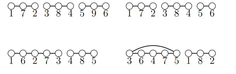
When \(k=5\), the cliques in \(S\) have orders 2, 2, 2, 1, 1, or 3, 2, 1, 1, 1. The latter is impossible since each component of \(\overline{G}\) has at most one 1-clique. In the former case, \(\overline{G}\) must be \(2P_{3}\cup K_{2}\), \(P_{5}\cup P_{3}\), or \(C_{5}\cup P_{3}\). In each case, it is easy to find an SL ordering that yields a 5-coloring of \(G\) (see the SL orderings on each \(\overline{G}\) above).
Now assume to the contrary that there is some \(k>4\) for which there is a HC graph for the SL algorithm with \(\chi\left(G\right)=k\) and order less than \(k+4\), and let \(k\) be the smallest value so that this occurs. Then \(G\) must have a dominating vertex \(v\). By Lemma 3.4, \(G-v\) is a HC graph for the SL algorithm with \(\chi\left(G\right)=k-1\) and order less than \(k+3\), a contradiction. ◻