
Throughout this paper, we consider the graph \(G = (V, E)\), where the vertex set is \(V\) and the edge set is \(E\). The graphs used in this study are simple graphs without loops or multiple edges. For a subset \(S \subseteq V\) and a vertex \(v \in V\), we use \(G[S]\) to represent the subgraph of \(G\) induced by \(S\). A vertex \(u\) that is adjacent to \(v\) is a neighbor of \(v\) for every \(v \in V\). All of \(v\)’s neighbors are included in the neighbor set of \(v\) in \(G\), which is represented by \(N_{G}(v)\). A vertex \(v\)’s degree is \(|N_{G}(v)|\), and it is represented as \(deg_{G}(v)\). Let \(m, n \geq 2\). The \(m \times n\) grid graph, denoted by \(G_{m,n} = (V,E)\), is an undirected graph whose vertex set is \(V = \{ v_{i,j} \mid 1 \leq i \leq m, \; 1 \leq j \leq n \}.\) The vertex in the grid’s \(i\)-th row and \(j\)-th column is represented by \(v_{i,j}\) in this case. Two vertices \(v_{i,j}\) and \(v_{k,\ell}\) are adjacent if and only if they are adjacent either horizontally or vertically; that is, \(\{v_{i,j}, v_{k,\ell}\} \in E\) precisely when \(i = k\) and \(|j – \ell| = 1\), or \(j = \ell\) and \(|i – k| = 1\). A subset \(D \subseteq V(G)\) is called a dominating set of \(G\) if every vertex in \(V(G)\setminus D\) has a neighbor in \(D\). If the subset \(G[F]\) induced by a dominating set \(F\) of \(G\) has a \(2\)-factor, then \(F\) is called a \(2\)-factored dominating set of \(G\). This means that if \(F\) is a \(2\)-factored dominating set or \(2\)fd-set, then
every vertex in \(V \setminus F\) is adjacent to a vertex in \(F\) and
\(G[F]\) has \(2\)-factor (a cycle or a disjoint union of cycles).
Numerous studies on the domination numbers of grid graph classes have been published, including [1, 4, 5, 8, 13, 14]. Domination parameters in grid graphs have been studied since Chang and Wu’s initial foundational work [3], in which they looked at domination numbers in grids. Grid graphs, which are classical and well researched graphs that represent spatial structures, planar graphs, and computational meshes, are defined as Cartesian products of paths [12]. For combinatorial enumeration tasks, grid graphs are perfect because of their regular and recursive structure. Paired domination was first formally described by Haynes et al. [10] and has since been studied in a variety of graphs, such as trees, cycles, Cartesian products, and grid graphs. In addition to being mathematically interesting because of their regular structure, grid graphs can be used to represent a variety of real-world systems, including VLSI circuit designs, image grids, city block models, and computational meshes. Later extensions have investigated paired domination, total domination, and independent domination [6]. The enumeration of \(2\)-factored dominating sets is still a relatively unexplored subject, despite the substantial study of classical domination in grid graphs [2], which presents a rich environment for new theoretical conclusions and real-world applications. The enumeration of paired or \(2\)-factored dominating sets, particularly in small grids, has received less attention than the extensive work on domination numbers in grid graphs in [3, 9, 15]. Combinatorial optimization, discrete dynamical systems, and combinatorial game theory are some of the new fields which help from the study of \(2\)-factored dominating sets and paired dominating sets in grid graphs. Tutte’s Factor Theorem [16] and the theory of matching and covering [3, 6] are two important examples of classical graph theory that have deep origins in the study of \(2\)-factor related structures. Combinatorial games, such as the Game of Amazons, which simulate territory control on a grid board, are based on the notions of domination and influence spread. According to research by Hung et al. [11], paired domination in extended hypergrid graphs of a generalization of grid graphs is computationally difficult yet essential for system design optimization. Yang [18] investigated this in the context of king grids, which have coverage and movement patterns that resemble the chess king. Even though domination in grids has been studied extensively, there is still unexplored the research on listing \(2\)-factored dominanting sets. The additional cycle requirements that must be satisfied in the induced subgraph make this task combinatorially difficult. In addition to expanding our theoretical knowledge of domination variants, this research improves real-world applications in robotics, surveillance, and informatin sharing-particularly in situations where redundancy and resilience are critical. Firstly, We present our theorems concerning the enumeration of \(2\)-factored dominanting sets in \(m \times n\) grid graphs when \(m \in \{2,3,4\}\). We then establish the asymptotic behavior of their growth rates as the grid graph’s size increases, study their structural recurrences, and create generating functions that accurately enumerate these sets.
In this section, we present the theorems concerning the enumeration of \(2\)-factored dominating sets in \(m \times n\) grid graphs when \(m \in \{2,3,4\}\). These theorems establish generating functions of counting the number of \(2\)-factored dominating sets in \(2 \times n\), \(3 \times n\) and \(4 \times n\) grid graphs.
Theorem 2.1. Let \(a_n\) be the number of \(2\)-factored dominating sets in the \(2 \times n\) grid graph. Then the generating function \(A(x)=\sum\limits_{n\ge2} a_nx^n\) satisfies \[A(x)=\frac{x^2+2x^3+x^4}{1-x-x^2-x^3}.\]
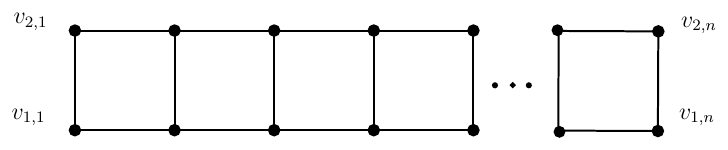
Proof. We consider \(G_{2,n}\) as the \(2 \times n\) grid graph, which is the particular case of the \(m \times n\) grid graph with exactly two rows and \(n\) columns. Its vertex set is \(V(G_{2,n})=\{v_{i,j}\mid i\in\{1,2\},\ 1\le j\le n\},\) where \(v_{i,j}\) denotes the vertex in the \(i\)-th row and \(j\)-th column. Two vertices \(v_{i,j}\) and \(v_{k,\ell}\) are adjacent if and only if they are adjacent horizontally or vertically; that is, \(\{v_{i,j},v_{k,\ell}\}\in E(G_{2,n})\) whenever either \(i=k\) and \(|j-\ell|=1\), or \(j=\ell\) and \(|i-k|=1\). Figure 1 illustrates the graph \(G_{2,n}\).
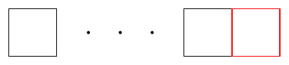
Let \(\widetilde{a}_n\) denote the number of \(2\)-factored dominating sets containing both vertices \(v_{1,n}\) and \(v_{2,n}\) of the last column.
Let \(\widehat{a}_n\) denote the number of \(2\)-factored dominating sets in which the cycle containing a vertex of the last column continues to the left.
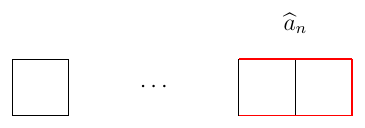
The initial values are \(a_0=a_1=\widetilde{a}_0=\widetilde{a}_1=\widehat{a}_0=\widehat{a}_1=0.\) It is easily verified that the graph \(G_{2,2}\) is a \(4\)-cycle, and hence \(a_2=1,\widetilde{a}_2=1, \widehat{a}_2=0.\) Similarly, the graph \(G_{2,3}\) has three \(2\)-factored dominating sets, giving \(a_3=3, \widetilde{a}_3=2, \widehat{a}_3=1.\) We define the generating functions \(A(x)=\sum\limits_{n\ge 2} a_n x^n, \widetilde{A}(x)=\sum\limits_{n\ge 2}\widetilde{a}_n x^n,\) and \(\widehat{A}(x)=\sum\limits_{n\ge 2}\widehat{a}_n x^n.\) We now derive the following equations: \[(1-x^2)A(x) = x^2+x^3+2x\widetilde{A}(x). \tag{1}\] \[(1-x)\widetilde{A}(x) = x^2A(x)+x^2+x^3.\tag{2}\] \[\widehat{A}(x)=x\widetilde{A}(x). \tag{3}\]
Proof of Eq. (1). We now consider \(a_n\), the number of \(2\)-factored dominating sets in \(G_{2,n}\). We distinguish three possible cases according to the structure of the cycle containing the vertices of the last column.
Case 1. The edge \(v_{1,n}v_{2,n}\) is not contained in any cycle of the induced \(2\)-factor.
In this case, deleting the last column of \(G_{2,n}\) yields a \(2\)-factored dominating set of \(G_{2,n-1}\) counted by \(\widetilde{a}_{n-1}\). Conversely, every \(2\)-factored dominating set counted by \(\widetilde{a}_{n-1}\) can be extended uniquely by adding a new column whose vertices do not belong to any cycle of the induced \(2\)-factor. Therefore, this case contributes \(\widetilde{a}_{n-1}\).
Case 2. The cycle containing the edge \(v_{1,n}v_{2,n}\) is the \(4\)-cycle induced by the vertices \(v_{1,n-1},\, v_{2,n-1},\,v_{1,n},\, v_{2,n}.\)
Deleting columns \(n-1\) and \(n\) yields a \(2\)-factored dominating set of \(G_{2,n-2}\). Conversely, every \(2\)-factored dominating set of \(G_{2,n-2}\) can be extended by adjoining the \(4\)-cycle induced by these four vertices. Therefore, this case contributes \(a_{n-2}\).
Case 3. The cycle containing the vertices \(v_{1,n}\) and \(v_{2,n}\) is not the \(4\)-cycle induced by columns \(n-1\) and \(n\), but is a cycle of length at least \(6\).
After deleting the last column and joining the edge \(v_{1,n-1}v_{2,n-1}\), we obtain a \(2\)-factored dominating set counted by \(\widetilde{a}_{n-1}\). Conversely, every \(2\)-factored dominating set counted by \(\widetilde{a}_{n-1}\) can be extended by adjoining column \(n\) so that \(v_{1,n}\) and \(v_{2,n}\) belong to a cycle that is not contained in columns \(n-1\) and \(n\). Therefore, this case contributes \(\widetilde{a}_{n-1}\).
From the three cases, we have \[a_n=a_{n-2}+2\widetilde{a}_{n-1}, \qquad n\ge 4.\]
We multiply by \(x^n\) and sum over \(n\ge 4\), we obtain \[\sum\limits_{n\ge4}a_nx^n = \sum\limits_{n\ge4}a_{n-2}x^n + 2\sum\limits_{n\ge4}\widetilde{a}_{n-1}x^n.\]
Thus, \[A(x)-a_2x^2-a_3x^3 = x^2A(x) + 2x\bigl(\widetilde{A}(x)-\widetilde{a}_2x^2\bigr).\]
Thus, we obtain \(A(x)-x^2-3x^3 = x^2A(x) + 2x\widetilde{A}(x) – 2x^3.\)
Hence, \[(1-x^2)A(x) = x^2+x^3+2x\widetilde{A}(x).\]
This proves Eq. (1). ◻
Proof of Eq. (2). We consider \(\widetilde{a}_n\), the number of \(2\)-factored dominating sets containing both vertices \(v_{1,n}\) and \(v_{2,n}\) of the last column. We distinguish two possible cases according to the structure of the cycle containing the vertices of the last column.
Case 1. The cycle containing the vertices \(v_{1,n}\) and \(v_{2,n}\) is the \(4\)-cycle induced by columns \(n-1\) and \(n\).
In this case, removing columns \(n-1\) and \(n\) leaves a \(2\)-factored dominating set of \(G_{2,n-2}\). Conversely, every \(2\)-factored dominating set of \(G_{2,n-2}\) can be extended by adjoining the \(4\)-cycle induced by columns \(n-1\) and \(n\). Hence, this case contributes \(a_{n-2}\).
Case 2. The cycle containing the vertices \(v_{1,n}\) and \(v_{2,n}\) extends beyond columns \(n-1\) and \(n\).
Deleting the last column and joining the vertices \(v_{1,n-1}\) and \(v_{2,n-1}\) yields a \(2\)-factored dominating set of \(G_{2,n-1}\) counted by \(\widetilde{a}_{n-1}\). Conversely, every \(2\)-factored dominating set counted by \(\widetilde{a}_{n-1}\) can be extended by adjoining column \(n\) so that the cycle containing \(v_{1,n}\) and \(v_{2,n}\) extends beyond columns \(n-1\) and \(n\). Therefore, this case contributes \(\widetilde{a}_{n-1}\).
From the two cases, we have \[\widetilde{a}_n=a_{n-2}+\widetilde{a}_{n-1}, \qquad n\ge 4.\]
Multiplying by \(x^n\) and summing over \(n\ge 4\), we obtain \[\sum\limits_{n\ge4}\widetilde{a}_nx^n = \sum\limits_{n\ge4}a_{n-2}x^n + \sum\limits_{n\ge4}\widetilde{a}_{n-1}x^n.\]
Thus, \[\widetilde{A}(x)-\widetilde{a}_2x^2-\widetilde{a}_3x^3 = x^2A(x) + x\bigl(\widetilde{A}(x)-\widetilde{a}_2x^2\bigr).\]
we obtain \[\widetilde{A}(x)-x^2-2x^3 = x^2A(x)+x\widetilde{A}(x)-x^3.\]
Therefore, \[(1-x)\widetilde{A}(x) = x^2A(x)+x^2+x^3.\] This proves Eq. (2). ◻
Proof of Eq. (3). Next, we consider \(\widehat{a}_n\), the number of \(2\)-factored dominating sets in which the cycle containing \(v_{1,n}\) and \(v_{2,n}\) extends beyond columns \(n-1\) and \(n\).
Case 1. The cycle containing \(v_{1,n}\) and \(v_{2,n}\) extends beyond columns \(n-1\) and \(n\).
Deleting the last column and joining the vertices \(v_{1,n-1}\) and \(v_{2,n-1}\) yields a \(2\)-factored dominating set of \(G_{2,n-1}\) counted by \(\widetilde{a}_{n-1}\). Conversely, every \(2\)-factored dominating set counted by \(\widetilde{a}_{n-1}\) can be extended uniquely by adjoining column \(n\) so that the cycle containing \(v_{1,n}\) and \(v_{2,n}\) extends beyond columns \(n-1\) and \(n\). Therefore, this case contributes \(\widetilde{a}_{n-1}\).
For \[\widehat{a}_n=\widetilde{a}_{n-1}, \qquad n\ge 4.\]
We multiply by \(x^n\) and sum over \(n\ge 4\):
\[\sum\limits_{n\ge4}\widehat{a}_n x^n = \sum\limits_{n\ge4}\widetilde{a}_{n-1}x^n.\]
Then \(\widehat{A}(x)-\widehat{a}_2x^2-\widehat{a}_3x^3 = x\bigl(\widetilde{A}(x)-\widetilde{a}_2x^2\bigr).\)
we obtain \[\widehat{A}(x)-x^3 = x\widetilde{A}(x)-x^3.\]
Hence, \[\widehat{A}(x)=x\widetilde{A}(x).\]
This proves Eq. (3). ◻
Solving 1, 2 and 3, we obtain \[A(x) = \frac{x^2+2x^3+x^4}{1-x-x^2-x^3}.\]
This proves Theorem 2.1. ◻
Lemma 2.2. Let \(F(x)=\frac{P(x)}{Q(x)},\) where \(P(x)\) and \(Q(x)\) are polynomials. Suppose that \(\rho\) is the unique dominant zero of \(Q(x)\), that \(\rho\) is a simple zero of \(Q(x)\), and that \(P(\rho)\neq 0\). Then \[[x^n]F(x) \sim -\frac{P(\rho)}{Q'(\rho)}\,\rho^{-n-1}.\]
The result is a standard consequence of the asymptotic theory of rational generating functions; see, for example, [7].
Theorem 2.3. If \(a_n\) is the number of \(2\)fd-sets of \(G_{2,n}\) and the generating function of the sequence \(\{a_n\}_{n \ge 0}\) is \[A(x) = \sum\limits_{n \ge 0} a_n x^n = \frac{x^2+2x^3+x^4}{1-x-x^2-x^3},\] then the sequence \(\{a_n\}\) grows exponentially and satisfies \[a_n \sim \frac{0.236840}{(0.543689)^{\,n+1}} \quad \text{as } n \to \infty.\]
Proof. The generating function \[A(x) = \frac{x^2 + 2x^3 + x^4}{1 – x – x^2 – x^3},\] has denominator \(Q(x) = 1 – x – x^2 – x^3\). The singularities of \(A(x)\) are the roots of \(Q(x)=0\). The dominant singularity is the unique real root \(\rho \approx 0.543689,\) and the other roots satisfy \(|x| > \rho\): \(x_{2,3} \approx -0.771844 \pm 1.11514i, \qquad |x_{2,3}| \approx 1.356.\) Thus, \(P(\rho) = \rho^2 + 2\rho^3 + \rho^4 \neq 0.\) Near \(x = \rho\), \[A(x) \sim \frac{\rho^2 + 2\rho^3 + \rho^4}{-Q'(\rho)} \cdot \frac{1}{x – \rho},\] so the residue is \[r = \frac{\rho^2 + 2\rho^3 + \rho^4}{-Q'(\rho)} \approx -0.236840.\]
Therefore, by Lemma 2.2 and singularity analysis [7, 17], \[a_n \sim \frac{0.236840}{(0.543689)^{n+1}} \quad \text{as } n \to \infty.\]
This proves the theorem. ◻
Theorem 2.4. Let \(b_n\) be the number of \(2\)-factored dominating sets in a \(3 \times n\) grid graph. Then the generating function \(B(x)=\sum\limits_{n\geq2} b_nx^n\) satisfies \[\begin{aligned} B(x) = \frac{x^2(3-x)} {1-2x-x^2-x^4}. \end{aligned}\]
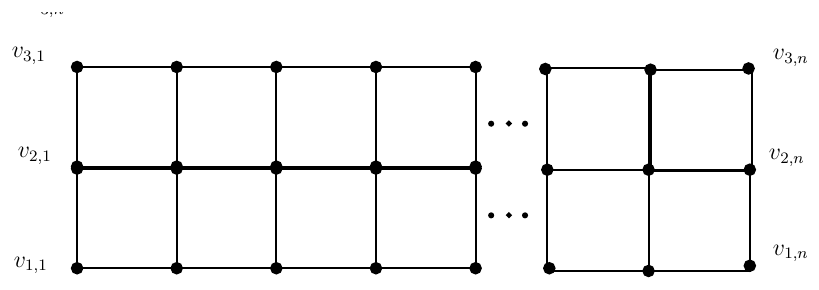
Proof. We consider the \(3 \times n\) grid graph \(G_{3,n}\), which consists of three rows and \(n\) columns. Its vertex set is \(V(G_{3,n})=\{v_{i,j}\mid i\in\{1,2,3\},\ 1\le j\le n\},\) where two vertices are adjacent whenever they are horizontally or vertically adjacent in the grid. Figure 4 illustrates the graph \(G_{3,n}\).
Here, \(b_n\) denotes the number of \(2\)-factored dominating sets in \(G_{3,n}\). Let \(\widetilde{b}_n\) denote the number of \(2\)-factored dominating sets in which the vertices \(v_{1,n}\) and \(v_{2,n}\), or the vertices \(v_{2,n}\) and \(v_{3,n}\), belong to the \(4\)-cycle induced by columns \(n-1\) and \(n\).
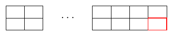
Let \(b_n’\) denote the number of \(2\)-factored dominating sets in which the cycle containing the last column is a longer cycle; that is, a cycle of length greater than \(4\) containing the vertical edges \(v_{1,n}v_{2,n}\) and \(v_{2,n}v_{3,n}\).
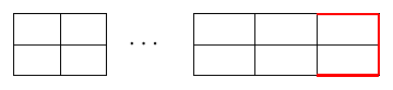
The initial values are \(b_0=b_1=\widetilde{b}_0=\widetilde{b}_1=b’_0=b’_1=0.\) For \(n=2\), there are exactly three \(2\)-factored dominating sets of \(G_{3,2}\), namely two \(4\)-cycles and one outer \(6\)-cycle. Hence \(b_2=3, \widetilde{b}_2=1,b’_2=1.\) For \(n=3\), the graph \(G_{3,3}\) has five \(2\)-factored dominating sets. Hence \(b_3=5.\) We define the generating functions \(B(x)=\sum\limits_{n\ge2} b_nx^n, \widetilde{B}(x)=\sum\limits_{n\ge2} \widetilde{b}_nx^n, B'(x)=\sum\limits_{n\ge2} b’_nx^n.\) We now derive the following equations: \[(1-x^2)B(x) = 3x^2 + 2x\widetilde{B}(x) + 3xB'(x), \tag{4}\] \[(1-x)\widetilde{B}(x)=x^2+x^2B(x)+xB'(x), \tag{5}\] \[(1-x)B'(x) = x^2+x\widetilde{B}(x). \tag{6}\]
Proof of Eq. (4). We now consider \(b_n\), the number of \(2\)-factored dominating sets in \(G_{3,n}\). We distinguish the following cases according to the structure of the cycle containing a vertex of the last column.
Case 1. The cycle contains the edges \(v_{1,n-1}v_{1,n}\), \(v_{1,n}v_{2,n}\), \(v_{2,n}v_{3,n}\), and \(v_{3,n}v_{3,n-1}\). We count the number of \(2\)-factored dominating sets arising from the following subcases.
Subcase 1.1. The cycle contains the edges \(v_{2,n-2}v_{2,n-1}\), \(v_{2,n-1}v_{1,n-1}\), \(v_{1,n-1}v_{1,n}\), \(v_{1,n}v_{2,n}\), \(v_{2,n}v_{3,n}\), \(v_{3,n}v_{3,n-1}\), and \(v_{3,n-1}v_{3,n-2}\). Deleting the last column and adding the edge \(v_{2,n-1}v_{3,n-1}\) results in a \(2\)-factored dominating set counted by \(\widetilde{b}_{n-1}\). Hence, this subcase contributes \(\widetilde{b}_{n-1}\).
Subcase 1.2. The cycle contains the edges \(v_{1,n-2}v_{1,n-1}\), \(v_{1,n-1}v_{1,n}\), \(v_{1,n}v_{2,n}\), \(v_{2,n}v_{3,n}\), \(v_{3,n}v_{3,n-1}\), and \(v_{3,n-1}v_{3,n-2}\). Deleting the last column and joining \(v_{2,n-1}v_{3,n-1}\) and \(v_{2,n-1}v_{1,n-1}\) obtains a \(2\)-factored dominating set counted by \(b’_{n-1}\). Therefore, this subcase contributes \(b’_{n-1}\).
Subcase 1.3. The cycle is the \(6\)-cycle containing the edges \(v_{1,n-1}v_{1,n}\), \(v_{1,n}v_{2,n}\), \(v_{2,n}v_{3,n}\), \(v_{3,n}v_{3,n-1}\), \(v_{3,n-1}v_{2,n-1}\), and \(v_{2,n-1}v_{1,n-1}\). Deleting columns \(n-1\) and \(n\) produces a \(2\)-factored dominating set counted by \(b_{n-2}\). Therefore, this subcase contributes \(b_{n-2}\).
From the three subcases, there are \(\widetilde{b}_{n-1} + b’_{n-1} + b_{n-2}\).
Case 2. The cycle contains either the edges \(v_{1,n-2}v_{1,n-1}\), \(v_{1,n-1}v_{1,n}\), \(v_{1,n}v_{2,n}\), \(v_{2,n}v_{2,n-1}\), \(v_{2,n-1}v_{3,n-1}\), and \(v_{3,n-1}v_{3,n-2}\), or the edges \(v_{1,n-2}v_{1,n-1}\), \(v_{1,n-1}v_{2,n-1}\), \(v_{2,n-1}v_{2,n}\), \(v_{2,n}v_{3,n}\), \(v_{3,n}v_{3,n-1}\), and \(v_{3,n-1}v_{3,n-2}\). In either case, deleting the last column and joining \(v_{1,n-1}\)\(v_{2,n-1}\) or \(v_{2,n-1}\)\(v_{3,n-1}\) produces a \(2\)-factored dominating set counted by \(b’_{n-1}\). Therefore, this case contributes \(b’_{n-1}\).
Case 3. The cycle contains the edges \(v_{1,n-2}v_{1,n-1}\), \(v_{1,n-1}v_{2,n-1}\), \(v_{2,n-1}v_{3,n-1}\), and \(v_{3,n-1}v_{3,n-2}\). Deleting the last column and joining the edges \(v_{1,n-1}\)\(v_{2,n-1}\) and \(v_{2,n-1}\)\(v_{3,n-1}\) produces a \(2\)-factored dominating set counted by \(b’_{n-1}\). Therefore, this case contributes \(b’_{n-1}\).
Case 4. The cycle contains the edges \(v_{1,n-2}v_{1,n-1}\), \(v_{1,n-1}v_{1,n}\), \(v_{1,n}v_{2,n}\), and \(v_{2,n}v_{2,n-1}\). The number of \(2\)-factored dominating sets arising from this structure is counted by \(\widetilde{b}_{n-1}\). Therefore, this case contributes \(\widetilde{b}_{n-1}\).
From the four cases, we have \[b_n = 2\widetilde{b}_{n-1} + 3b’_{n-1} + b_{n-2}, \qquad n\ge 3.\]
We multiply by \(x^n\) and sum over \(n\ge3\). Then \[\sum\limits_{n\geq 3}^{\infty} b_nx^n = 2\sum\limits_{n\geq 3}^{\infty}\widetilde{b}_{n-1}x^n + 3\sum\limits_{n\geq 3}^{\infty}b’_{n-1}x^n + \sum\limits_{n \geq 3}^{\infty}b_{n-2}x^n.\]
Thus, \[B(x)-b_2x^2 = 2x\widetilde{B}(x) + 3xB'(x) + x^2B(x).\]
Thus, we obtain \(B(x)-3x^2 = 2x\widetilde{B}(x) + 3xB'(x) + x^2B(x).\)
Hence, \[(1-x^2)B(x) = 3x^2 + 2x\widetilde{B}(x) + 3xB'(x).\]
This proves Eq. (4). ◻
Proof of Eq. (5). We now consider \(\widetilde{b}_n\), the number of \(2\)-factored dominating sets in which the vertices \(v_{1,n}\) and \(v_{2,n}\), or symmetrically the vertices \(v_{2,n}\) and \(v_{3,n}\), belong to the \(4\)-cycle induced by columns \(n-1\) and \(n\). We distinguish three possible cases according to the position of this \(4\)-cycle.
Case 1. The cycle is the \(4\)-cycle containing the edges \(v_{1,n-1}v_{1,n}\), \(v_{1,n}v_{2,n}\), \(v_{2,n}v_{2,n-1}\), and \(v_{2,n-1}v_{1,n-1}\). Deleting columns \(n-1\) and \(n\) produces a \(2\)-factored dominating set counted by \(b_{n-2}\). Therefore, this case contributes \(b_{n-2}\).
Case 2. The cycle contains the edges \(v_{1,n-2}v_{1,n-1}\), \(v_{1,n-1}v_{1,n}\), \(v_{1,n}v_{2,n}\), \(v_{2,n}v_{2,n-1}\), \(v_{2,n-1}v_{3,n-1}\), and \(v_{3,n-1}v_{3,n-2}\). Deleting the last column and joining \(v_{1,n-1}\) and \(v_{2,n-1}\) produces a \(2\)-factored dominating set counted by \(b’_{n-1}\). Therefore, this case contributes \(b’_{n-1}\).
Case 3. The cycle contains the edges \(v_{1,n-2}v_{1,n-1}\), \(v_{1,n-1}v_{1,n}\), \(v_{1,n}v_{2,n}\), and \(v_{2,n}v_{2,n-1}\). Deleting the last column and joining \(v_{1,n-1}\) and \(v_{2,n-1}\) produces a \(2\)-factored dominating set counted by \(\widetilde{b}_{n-1}\). Therefore, this case contributes \(\widetilde{b}_{n-1}\).
From the three cases, we have
\[\widetilde{b}_{n} = b_{n-2} + b’_{n-1} + \widetilde{b}_{n-1}, \qquad n\ge3.\]
We multiply by \(x^n\) and sum over all \(n\ge3\). Then
\[\sum\limits_{n\geq 3}^{\infty}\widetilde{b}_{n}x^{n} = \sum\limits_{n\geq 3}^{\infty}b_{n-2}x^{n} + \sum\limits_{n\geq 3}^{\infty}b’_{n-1}x^{n} + \sum\limits_{n\geq 3}^{\infty}\widetilde{b}_{n-1}x^{n}.\]
Thus, \[\widetilde{B}(x)-\widetilde{b}_2x^2 = x^2B(x) + xB'(x) + x\widetilde{B}(x).\]
Thus, we obtain \(\widetilde{B}(x)-x^2 = x^2B(x) + xB'(x) + x\widetilde{B}(x).\)
Therefore, \[(1-x)\widetilde{B}(x) = x^2B(x) + x^2 + xB'(x).\] This proves Eq. (5). ◻
Proof of Eq. (6). We now consider \(b_n’\), the number of \(2\)-factored dominating sets in which the cycle containing the last column is a longer cycle; that is, a cycle of length greater than \(4\) containing the vertical edges \(v_{1,n}v_{2,n}\) and \(v_{2,n}v_{3,n}\). We distinguish four possible cases according to the structure of this cycle.
Case 1. The cycle contains the edges \(v_{1,n-2}v_{1,n-1}\), \(v_{1,n-1}v_{1,n}\), \(v_{1,n}v_{2,n}\), \(v_{2,n}v_{3,n}\), \(v_{3,n}v_{3,n-1}\), \(v_{3,n-1}v_{2,n-1}\), and \(v_{2,n-1}v_{2,n-2}\), or the edges \(v_{2,n-2}v_{2,n-1}\), \(v_{2,n-1}v_{1,n-1}\), \(v_{1,n-1}v_{1,n}\), \(v_{1,n}v_{2,n}\), \(v_{2,n}v_{3,n}\), \(v_{3,n}v_{3,n-1}\), and \(v_{3,n-1}v_{3,n-2}\). Deleting the last column and joining by the edges \(v_{1,n-1}v_{2,n-1}\) and \(v_{2,n-1}v_{3,n-1}\). Hence, the graph reduces to a counted by \(\widetilde{b}_{n-1}\).
Case 2. The cycle contains the edges \(v_{1,n-2}v_{1,n-1}\), \(v_{1,n-1}v_{1,n}\), \(v_{1,n}v_{2,n}\), \(v_{2,n}v_{3,n}\), \(v_{3,n}v_{3,n-1}\), and \(v_{3,n-1}v_{3,n-2}\). After deleting the last column and joining the remaining vertices by the edges \(v_{1,n-1}v_{2,n-1}\) and \(v_{2,n-1}v_{3,n-1}\), the resulting configuration is counted by \(b’_{n-1}\). Hence, this case contributes \(b’_{n-1}\).
From the two cases, we have \[b’_n=\widetilde{b}_{n-1}+b’_{n-1}, \qquad n\ge 3.\]
For \(n\ge 3\), we multiply \(x^n\) throughout the above equation and sum over all \(n\). Then \[\sum\limits_{n\geq 3}^{\infty} b’_n x^n = \sum\limits_{n \geq 3}^{\infty} \widetilde{b}_{n-1}x^n +\sum\limits_{n \geq 3}^{\infty} b’_{n-1}x^n.\]
This implies that \[B'(x)-b’_0-b’_1x-b’_2x^2 = x\bigl(\widetilde{B}(x)-\widetilde{b}_0-\widetilde{b}_1x\bigr) + x\bigl(B'(x)-b’_0-b’_1x\bigr).\]
Hence, \[B'(x)-x^2 = x\widetilde{B}(x)+xB'(x).\]
Therefore, \[(1-x)B'(x) = x^2 + x\widetilde{B}(x).\]
This proves Eq. (6). ◻
By Eqs. (4), (5) and (6), it can be solved that \[\begin{aligned} B(x) = \frac{x^2(3-x)} {1-2x-x^2-x^4}. \end{aligned}\]
This proves Theorem 2.4. ◻
We investigate the dominant asymptotic behavior associated with \(B(x)\). The following is attained since the dominant singularity is approximately \(0.40470\).
Theorem 2.5. If \(b_n\) is the number of \(2\)fd-sets of \(G_{3,n}\) and the generating function of the sequence \(\{b_n\}_{n \ge 0}\) is \[B(x) = \sum\limits_{n \ge 0} b_n x^n = \frac{x^2(3-x)}{1-2x-x^2-x^4},\] then the sequence \(\{b_n\}\) grows exponentially and satisfies \[b_n \sim \frac{0.138253}{(0.40470)^{\,n+1}} \quad \text{as } n \to \infty.\]
Proof. The generating function \[B(x) = \frac{3x^2 – x^3}{1-2x-x^2-x^4},\] has denominator \(Q(x) = 1 – 2x – x^2 – x^4\). The singularities of \(B(x)\) are the roots of \(Q(x)=0\). The dominant singularity is the unique real root \(\rho \approx 0.40470,\) and the other roots satisfy \(|x| > \rho\): \(x_2 \approx -1.1841, x_{3,4} \approx 0.38972 \pm 1.3910i.\) Thus, \(P(\rho) = 3\rho^2 – \rho^3 \neq 0.\) Near \(x = \rho\), \[B(x) \sim \frac{3\rho^2 – \rho^3}{-Q'(\rho)} \cdot \frac{1}{x – \rho},\] so the residue is \[r = \frac{3\rho^2 – \rho^3}{-Q'(\rho)} \approx -0.138253.\]
By Lemma 2.2 and singularity analysis [7, 17], \[b_n \sim \frac{0.138253}{(0.40470)^{n+1}} \quad \text{as } n \to \infty.\]
This proves the theorem. ◻
Theorem 2.6. Let \(c_n\) be the number of \(2\)-factored dominating sets in a \(4 \times n\) grid graph. Then the generating function \(C(x)=\sum\limits_{n\ge2} c_nx^n\) satisfies \[\begin{aligned} C(x) &= \frac{x^2\left(x^3+9x^2+9x+3\right)} {1-x-4x^2-7x^3-8x^4}, \end{aligned}\]
Proof. To prove Theorem 2.6, we consider the \(4 \times n\) grid graph \(G_{4,n}\), which consists of four rows and \(n\) columns. Its vertex set is \(V(G_{4,n})=\{v_{i,j}\mid i\in\{1,2,3,4\},\ 1\le j\le n\},\) where two vertices are adjacent whenever they are horizontally or vertically adjacent in the grid. Figure 7 illustrates the graph \(G_{4,n}\).
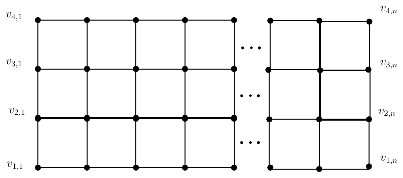
We define the generating function \(C(x)=\sum\limits_{n\ge2} c_nx^n, \widehat{C}(x)=\sum\limits_{n\ge2} \widehat{c}_nx^n,\) \(C'(x)=\sum\limits_{n\ge2} \\c_n’x^n, \widetilde{C}(x)=\sum\limits_{n\ge2} \widetilde{c}_nx^n.\) Here, \(c_n\) denotes the number of \(2\)-factored dominating sets in \(G_{4,n}\). \(\widehat{c}_n\) denotes the number of \(2\)-factored dominating sets in which the cycles of the induced \(2\)-factor contain the vertical edges \(v_{1,n}v_{2,n}\) and \(v_{3,n}v_{4,n}\) of the last column. \(c’_n\) denotes the number of \(2\)-factored dominating sets in which a cycle contains the vertices \(v_{1,n-1}\), \(v_{2,n-1}\), \(v_{3,n-1}\), \(v_{4,n-1}\), \(v_{1,n}\), \(v_{2,n}\), \(v_{3,n}\), and \(v_{4,n}\). In addition, we define \(c’_n\) as the number of \(2\)-factored dominating sets in which a cycle contains the vertices \(v_{1,n-1}\), \(v_{2,n-1}\), \(v_{3,n-1}\), \(v_{4,n-1}\), \(v_{1,n}\), \(v_{2,n}\), \(v_{3,n}\), and \(v_{4,n}\). The initial values are \(c_0=c_1=\widehat{c}_0=\widehat{c}_1=c’_0=c’_1=\widetilde{c}_0=\widetilde{c}_1=0.\) For \(n=2\), the graph \(G_{4,2}\) has three \(2\)-factored dominating sets. Hence, \(c_2=3,\widehat{c}_2=2,c’_2=1,\widetilde{c}_2=1.\) We now derive the following equations: \[(1-x^2)C(x) = 3x^2 + 4x\widehat{C}(x) + 3xC'(x) + x\widetilde{C}(x), \tag{7}\] \[\widehat{C}(x)-2x^2 = x^2C(x)+xC'(x), \tag{8}\] \[(1-x)C'(x) = x^2 + 3x\widehat{C}(x) + x^2C(x), \tag{9}\] \[\tilde{C}(x) = x^{2} + x^{2} C(x) + xC'(x) + 2x \widehat{C}(x), \tag{10}\]
Proof of Eq. (7). We now consider \(c_n\), the number of \(2\)-factored dominating sets in \(G_{4,n}\). We distinguish the following cases according to the structure of the cycle containing a vertex of the last column.
Case 1. The cycle containing vertices of the last column contains the edges \(v_{1,n-1}v_{1,n}\), \(v_{1,n}v_{2,n}\), \(v_{2,n}v_{3,n}\), \(v_{3,n}v_{4,n}\), and \(v_{4,n}v_{4,n-1}\). We distinguish the following subcases.
Subcase 1.1. The cycle contains either the edges \(v_{1,n-2}v_{1,n-1}\), \(v_{1,n-1}v_{1,n}\), \(v_{1,n}v_{2,n}\), \(v_{2,n}v_{3,n}\), \(v_{3,n}v_{4,n}\), \(v_{4,n}v_{4,n-1}\), \(v_{4,n-1}v_{3,n-1}\), and \(v_{3,n-1}v_{3,n-2}\), or the edges \(v_{2,n-2}v_{2,n-1}\), \(v_{2,n-1}v_{1,n-1}\), \(v_{1,n-1}v_{1,n}\), \(v_{1,n}v_{2,n}\), \(v_{2,n}v_{3,n}\), \(v_{3,n}v_{4,n}\), \(v_{4,n}v_{4,n-1}\), and \(v_{4,n-1}v_{4,n-2}\). Deleting the last column and joining the edges \(v_{1,n-1}v_{2,n-1}\) and \(v_{2,n-1}v_{3,n-1}\) or \(v_{4,n-1}v_{3,n-1}\) and \(v_{3,n-1}v_{2,n-1}\) results in a \(2\)-factored dominating set counted by \(\widehat{c}_{n-1}\). Therefore, this subcase contributes \(\widehat{c}_{n-1}\).
Subcase 1.2. The cycle contains the edges \(v_{1,n-2}v_{1,n-1}\), \(v_{1,n-1}v_{1,n}\), \(v_{1,n}v_{2,n}\), \(v_{2,n}v_{3,n}\), \(v_{3,n}v_{4,n}\), \(v_{4,n}v_{4,n-1}\), and \(v_{4,n-1}v_{4,n-2}\). Deleting the last column and joining \(v_{4,n-1}v_{3,n-1}\), \(v_{3,n-1}v_{2,n-1}\), and \(v_{2,n-1}v_{1,n-1}\), produces a \(2\)-factored dominating set counted by \(c’_{n-1}\). Therefore, this subcase contributes \(c’_{n-1}\).
Subcase 1.3. The cycle contains the edges \(v_{1,n-1}v_{1,n}\), \(v_{1,n}v_{2,n}\), \(v_{2,n}v_{3,n}\), \(v_{3,n}v_{4,n}\), \(v_{4,n}v_{4,n-1}\), \(v_{4,n-1}v_{3,n-1}\), \(v_{3,n-1}v_{2,n-1}\), and \(v_{2,n-1}v_{1,n-1}\). Deleting columns \(n-1\) and \(n\) produces a \(2\)-factored dominating set counted by \(c_{n-2}\). Therefore, this subcase contributes \(c_{n-2}\).
Subcase 1.4. The cycle contains the edges \(v_{2,n-2}v_{2,n-1}\), \(v_{2,n-1}v_{1,n-1}\), \(v_{1,n-1}v_{1,n}\), \(v_{1,n}v_{2,n}\), \(v_{2,n}v_{3,n}\), \(v_{3,n}v_{4,n}\), \(v_{4,n}v_{4,n-1}\), \(v_{4,n-1}v_{3,n-1}\), and \(v_{3,n-1}v_{3,n-2}\). Deleting the last column and joining the edge \(v_{2,n}v_{3,n}\) produces a \(2\)-factored dominating set counted by \(\widetilde{c}_{n-1}\). Therefore, this subcase contributes \(\widehat{c}_{n-1}\).
From the four subcases, there are 2\(\widehat{c}_{n-1} + c’_{n-1} + c_{n-2}\).
Case 2. The cycle contains either the edges \(v_{1,n-2}v_{1,n-1}\), \(v_{1,n-1}v_{1,n}\), \(v_{1,n}v_{2,n}\), \(v_{2,n}v_{3,n}\), \(v_{3,n}v_{3,n-1}\), \(v_{3,n-1}v_{4,n-1}\), and \(v_{4,n-1}v_{4,n-2}\), or the edges \(v_{1,n-2}v_{1,n-1}\), \(v_{1,n-1}v_{2,n-1}\), \(v_{2,n-1}v_{2,n}\), \(v_{2,n}v_{3,n}\), \(v_{3,n}v_{4,n}\), \(v_{4,n}v_{4,n-1}\), and \(v_{4,n-1}v_{4,n-2}\). Deleting the last column and joining \(v_{1,n-1}v_{2,n-1}\) and \(v_{2,n-1}v_{3,n-1}\) in the first configuration, or \(v_{4,n-1}v_{3,n-1}\) and \(v_{3,n-1}v_{2,n-1}\) in the second configuration, produces a \(2\)-factored dominating set counted by \(c’_{n-1}\). Therefore, this case contributes \(c’_{n-1}\).
Case 3. The cycle contains the edges \(v_{1,n-2}v_{1,n-1}\), \(v_{1,n-1}v_{2,n-1}\), \(v_{2,n-1}v_{3,n-1}\), \(v_{3,n-1}v_{4,n-1}\), and \(v_{4,n-1}v_{4,n-2}\). Deleting the last column and joining \(v_{1,n-1}v_{2,n-1}\), \(v_{2,n-1}v_{3,n-1}\), and \(v_{3,n-1}v_{4,n-1}\) obtains a \(2\)-factored dominating set counted by \(c’_{n-1}\). Therefore, this case contributes \(c’_{n-1}\).
Case 4. The cycle contains either the edges \(v_{1,n-2}v_{1,n-1}\), \(v_{1,n-1}v_{1,n}\), \(v_{1,n}v_{2,n}\), \(v_{2,n}v_{3,n}\), \(v_{3,n}v_{3,n-1}\), and \(v_{3,n-1}v_{3,n-2}\), or the edges \(v_{2,n-2}v_{2,n-1}\), \(v_{2,n-1}v_{2,n}\), \(v_{2,n}v_{3,n}\), \(v_{3,n}v_{4,n}\), \(v_{4,n}v_{4,n-1}\), and \(v_{4,n-1}v_{4,n-2}\). Deleting the last column and joining \(v_{1,n-1}v_{2,n-1}\) and \(v_{2,n-1}v_{3,n-1}\), or \(v_{4,n-1}v_{3,n-1}\) and \(v_{3,n-1}v_{2,n-1}\), yields a \(2\)-factored dominating set counted by \(\widehat{c}_{n-1}\). Therefore, this subcase contributes \(\widehat{c}_{n-1}\).
Case 5. The cycle continues to the left through the second and third rows and contains the edges \(v_{2,n-2}v_{2,n-1}\), \(v_{2,n-1}v_{2,n}\), \(v_{2,n}v_{3,n}\), \(v_{3,n}v_{3,n-1}\), and \(v_{3,n-1}v_{3,n-2}\). Deleting the last column and joining the edge \(v_{2,n-1}v_{3,n-1}\) produces a \(2\)-factored dominating set counted by \(\widetilde{c}_{n-1}\). Therefore, this case contributes \(\widetilde{c}_{n-1}\).
Case 6. The cycle includes the edges \(v_{1, n-2}v_{1, n-1}\), \(v_{1, n-1}v_{2,n-1}\), \(v_{2,n-1}v_{2,n}\), \(v_{2,n}v_{3,n}\), \(v_{3,n}v_{3, n-1}\), \(v_{3,n-1}v_{4, n-1}\) and \(v_{4,n-1}v_{4,n-2}\). The number of \(2\)-factored dominating sets in this case contributes \(c’_{n-1}\).
Case 7. The first cycle contains the edges \(v_{1,n-2}v_{1,n-1}\), \(v_{1,n-1}v_{1,n}\), \(v_{1,n}v_{2,n}\), \(v_{2,n}v_{2,n-1}\), and \(v_{2,n-1}v_{2,n-2}\), while the second cycle contains the edges \(v_{3,n-2}v_{3,n-1}\), \(v_{3,n-1}v_{3,n}\), \(v_{3,n}v_{4,n}\), \(v_{4,n}v_{4,n-1}\), and \(v_{4,n-1}v_{4,n-2}\). Deleting the last column and joining the edges \(v_{1,n-1}v_{2,n-1}\) and \(v_{3,n-1}v_{4,n-1}\) produces a \(2\)-factored dominating set counted by \(\widehat{c}_{n-1}\). Therefore, this case contributes \(\widehat{c}_{n-1}\).
From the seven cases, we have \(c_n = 4\widehat{c}_{n-1} + 3c’_{n-1} + c_{n-2} + \widetilde{c}_{n-1}, \quad n \ge 3.\)
For \(n \ge 3\), we multiply by \(x^n\) and sum over all \(n \ge 3\). Then
\[\sum\limits_{n \ge 3} c_n x^n = \sum\limits_{n \ge 3} 4\widehat{c}_{n-1} x^n + \sum\limits_{n \ge 3} 3c’_{n-1} x^n + \sum\limits_{n \ge 3} c_{n-2} x^n + \sum\limits_{n \ge 3} \widetilde{c}_{n-1} x^n.\]
Thus, \[C(x)-c_0-c_1x-c_2x^2 = 4x\bigl(\widehat{C}(x)-\widehat{c}_0-\widehat{c}_1x\bigr) + 3x\bigl(C'(x)-c’_0-c’_1x\bigr)\] \[+ x^2\bigl(C(x)-c_0\bigr) + x\bigl(\widetilde{C}(x)-\widetilde{c}_0-\widetilde{c}_1x\bigr).\]
Hence, \[C(x)-3x^2 = 4x\widehat{C}(x) + 3xC'(x) + x^2C(x) + x\widetilde{C}(x).\]
Therefore, \[(1-x^2)C(x) = 3x^2 + 4x\widehat{C}(x) + 3xC'(x) + x\widetilde{C}(x).\]
This proves Eq. (7). ◻
Proof of Eq. (8). We now consider \(\widehat{c}_n\), the number of \(2\)-factored dominating sets in which the cycles of the induced \(2\)-factor contain the edges \(v_{1,n}v_{2,n}\) and \(v_{3,n}v_{4,n}\) of the last column. We distinguish two possible cases according to the structure of these cycles.
pt Case 1. The first cycle contains the edges \(v_{1,n-2}v_{1,n-1}\), \(v_{1,n-1}v_{1,n}\), \(v_{1,n}v_{2,n}\), \(v_{2,n}v_{2,n-1}\), and \(v_{2,n-1}v_{2,n-2}\), while the second cycle contains the edges \(v_{3,n-2}v_{3,n-1}\), \(v_{3,n-1}v_{3,n}\), \(v_{3,n}v_{4,n}\), \(v_{4,n}v_{4,n-1}\), and \(v_{4,n-1}v_{4,n-2}\). Removing columns \(n-1\) and \(n\) yields a \(2\)-factored dominating set counted by \(c_{n-2}\). Conversely, every \(2\)-factored dominating set counted by \(c_{n-2}\) can be extended uniquely to a \(2\)-factored dominating set of this type. Therefore, this case contributes \(c_{n-2}\).
Case 2. The cycle contains the edges \(v_{1,n-2}v_{1,n-1}\), \(v_{1,n-1}v_{1,n}\), \(v_{1,n}v_{2,n}\), \(v_{2,n}v_{2,n-1}\), \(v_{2,n-1}v_{3,n-1}\), \(v_{3,n-1}v_{3,n}\), \(v_{3,n}v_{4,n}\), \(v_{4,n}v_{4,n-1}\), and \(v_{4,n-1}v_{4,n-2}\). Removing the last column and joining the edges \(v_{1,n-1}v_{2,n-1}\) and \(v_{3,n-1}v_{4,n-1}\) yields a \(2\)-factored dominating set counted by \(c’_{n-1}\). Conversely, every \(2\)-factored dominating set counted by \(c’_{n-1}\) can be extended uniquely to a \(2\)-factored dominating set of this type. Therefore, this case contributes \(c’_{n-1}\). From the two cases, we have \[\begin{aligned} \widehat{c}_n = c_{n-2}+c’_{n-1}, \qquad n\ge 3. \end{aligned}\]
We multiply \(x^n\) throughout the equation above and sum over all \(n\ge 3\). Then \[\begin{aligned} \sum\limits_{n\geq 3}^{\infty}\widehat{c}_n x^n &= \sum\limits_{n\geq 3}^{\infty}c_{n-2}x^n + \sum\limits_{n \geq 3}^{\infty}c’_{n-1}x^n . \end{aligned}\]
This implies that \[\begin{aligned} \widehat{C}(x)-\widehat{c}_0-\widehat{c}_1x-\widehat{c}_2x^2 &= x^2\left(C(x)-c_0\right) + x\left(C'(x)-c’_0-c’_1x\right). \end{aligned}\]
Hence, \[\begin{aligned} \widehat{C}(x)-2x^2 &= x^2C(x)+xC'(x). \end{aligned}\] Therefore, \[\begin{aligned} \widehat{C}(x) = 2x^2+x^2C(x)+xC'(x). \end{aligned}\] ◻
Proof of Eq. (9). We now consider \(c’_n\), the number of \(2\)-factored dominating sets in which a cycle contains the vertices \(v_{1,n-1}\), \(v_{2,n-1}\), \(v_{3,n-1}\), \(v_{4,n-1}\), \(v_{1,n}\), \(v_{2,n}\), \(v_{3,n}\), and \(v_{4,n}\). We distinguish five possible cases according to the structure of this cycle.
Case 1. The cycle contains the edges \(v_{1,n-2}v_{1,n-1}\), \(v_{1,n-1}v_{1,n}\), \(v_{1,n}v_{2,n}\), \(v_{2,n}v_{3,n}\), \(v_{3,n}v_{4,n}\), \(v_{4,n}v_{4,n-1}\), \(v_{4,n-1}v_{3,n-1}\), and \(v_{3,n-1}v_{3,n-2}\), or the edges \(v_{2,n-2}v_{2,n-1}\), \(v_{2,n-1}v_{1,n-1}\), \(v_{1,n-1}v_{1,n}\), \(v_{1,n}v_{2,n}\), \(v_{2,n}v_{3,n}\), \(v_{3,n}v_{4,n}\), \(v_{4,n}v_{4,n-1}\), and \(v_{4,n-1}v_{4,n-2}\). In either configuration, after deleting the vertices of the last column, we join the vertices in column \(n-1\) by adding the edges \(v_{1,n-1}v_{2,n-1}\), \(v_{2,n-1}v_{3,n-1}\), and \(v_{3,n-1}v_{4,n-1}\). Thus, we obtain a \(2\)-factored dominating set counted by \(\widehat{c}_{n-1}\).
Case 2. The cycle includes the edges \(v_{1,n-2}v_{1,n-1}\), \(v_{1,n-1}v_{1,n}\), \(v_{1,n}v_{2,n}\), \(v_{2,n}v_{3,n}\), \(v_{3,n}v_{4,n}\), \(v_{4,n}v_{4,n-1}\), \(v_{4,n-1}v_{3,n-1}\), \(v_{3,n-1}v_{2,n-1}\), and \(v_{2,n-1}v_{2,n-2}\). After deleting the vertices of the last column and adding the edges \(v_{1,n-1}v_{2,n-1}\), \(v_{2,n-1}v_{3,n-1}\), and \(v_{3,n-1}v_{4,n-1}\), we obtain a \(2\)-factored dominating set counted by \(\widehat{c}_{n-1}\). Therefore, this case contributes \(\widehat{c}_{n-1}\).
Case 3. The cycle contains the edges \(v_{1,n-2}v_{1,n-1}\), \(v_{1,n-1}v_{1,n}\), \(v_{1,n}v_{2,n}\), \(v_{2,n}v_{3,n}\), \(v_{3,n}v_{4,n}\), \(v_{4,n}v_{4,n-1}\), and \(v_{4,n-1}v_{4,n-2}\). After deleting the vertices of the last column and adding the edge \(v_{2,n-1}v_{3,n-1}\), we obtain a \(2\)-factored dominating set counted by \(c’_{n-1}\). Therefore, this case contributes \(c’_{n-1}\).
Case 4. The cycle is the \(8\)-cycle containing the edges \(v_{1,n-1}v_{1,n}\), \(v_{1,n}v_{2,n}\), \(v_{2,n}v_{3,n}\), \(v_{3,n}v_{4,n}\), \(v_{4,n}v_{4,n-1}\), \(v_{4,n-1}v_{3,n-1}\), \(v_{3,n-1}v_{2,n-1}\), and \(v_{2,n-1}v_{1,n-1}\). After deleting the last two columns, we obtain a \(2\)-factored dominating set counted by \(c_{n-2}\). Therefore, this case contributes \(c_{n-2}\).
Case 5. The cycle contains the edges \(v_{2,n-2}v_{2,n-1}\), \(v_{2,n-1}v_{1,n-1}\), \(v_{1,n-1}v_{1,n}\), \(v_{1,n}v_{2,n}\), \(v_{2,n}v_{3,n}\), \(v_{3,n}v_{4,n}\), \(v_{4,n}v_{4,n-1}\), \(v_{4,n-1}v_{3,n-1}\), and \(v_{3,n-1}v_{3,n-2}\). After deleting the vertices of the last column and adding the edges \(v_{1,n-1}v_{2,n-1}\), \(v_{2,n-1}v_{3,n-1}\), and \(v_{3,n-1}v_{4,n-1}\), we obtain a \(2\)-factored dominating set counted by \(\widehat{c}_{n-1}\). Therefore, this case contributes \(\widehat{c}_{n-1}\).
From the five cases, we have \[\begin{aligned} c’_n = 3\widehat{c}_{n-1} + c_{n-2} + c’_{n-1}, \qquad n\geq 3. \end{aligned}\]
We multiply \(x^n\) in the equation above and sum up all \(n\) for \(n\geq 3\). We have that \[\begin{aligned} \sum\limits_{n=3}^{\infty} c’_n x^n &= \sum\limits_{n=3}^{\infty}3\widehat{c}_{n-1}x^n + \sum\limits_{n=3}^{\infty}c_{n-2}x^n + \sum\limits_{n=3}^{\infty}c’_{n-1}x^n. \end{aligned}\]
This implies that \[\begin{aligned} C'(x)-c’_0-c’_1x-c’_2x^2 &= 3x\left(\widehat{C}(x)-\widehat{c}_0-\widehat{c}_1x\right) +x^2\left(C(x)-c_0\right)\\ &\quad +x\left(C'(x)-c’_0-c’_1x\right). \end{aligned}\]
Hence, \[\begin{aligned} C'(x)-x^2 &= 3x\widehat{C}(x) +x^2C(x) +xC'(x). \end{aligned}\]
Therefore, \[\begin{aligned} (1-x)C'(x) = x^2 + 3x\widehat{C}(x) + x^2C(x). \end{aligned}\]
This proves Eq. (9). ◻
Proof of Eq. (10). We now consider \(\widetilde{c}_n\), the number of \(2\)-factored dominating sets in which the vertices \(v_{2,n-1}\), \(v_{3,n-1}\), \(v_{2,n}\), and \(v_{3,n}\) belong to a \(4\)-cycle. We distinguish four possible cases according to the structure of the remaining cycles.
Case 1. The cycle contains the edges \(v_{2,n-1}v_{2,n}\), \(v_{2,n}v_{3,n}\), \(v_{3,n}v_{3,n-1}\), and \(v_{3,n-1}v_{2,n-1}\). After deleting the last two columns, we obtain a \(2\)-factored dominating set counted by \(c_{n-2}\). Therefore, this case contributes \(c_{n-2}\).
Case 2. The cycle contains the edges \(v_{1,n-2}v_{1,n-1}\), \(v_{1,n-1}v_{2,n-1}\), \(v_{2,n-1}v_{2,n}\), \(v_{2,n}v_{3,n}\), \(v_{3,n}v_{3,n-1}\), \(v_{3,n-1}v_{4,n-1}\), and \(v_{4,n-1}v_{4,n-2}\). After deleting the vertices of the last column and adding the edge \(v_{2,n-1}v_{3,n-1}\), we obtain a \(2\)-factored dominating set counted by \(c’_{n-1}\). Therefore, this case contributes \(c’_{n-1}\).
Case 3. The cycle contains the edges \(v_{2,n-2}v_{2,n-1}\), \(v_{2,n-1}v_{2,n}\), \(v_{2,n}v_{3,n}\), \(v_{3,n}v_{3,n-1}\), and \(v_{3,n-1}v_{4,n-1}\). After deleting the vertices of the last column and adding the edge \(v_{2,n-1}v_{3,n-1}\), we obtain a \(2\)-factored dominating set counted by \(\widehat{c}_{n-1}\). Therefore, this case contributes \(\widehat{c}_{n-1}\).
Case 4. The cycle includes the edges \(v_{1,n-1}v_{2,n-1}\), \(v_{2,n-1}v_{2,n}\), \(v_{2,n}v_{3,n}\), \(v_{3,n}v_{3,n-1}\) and \(v_{3,n-1}v_{3,n-2}\). The number of \(2\)-factored dominating sets in this case contributes \(\widetilde{c}_{n-1}\).
From the four cases, we have \[\begin{aligned} \tilde{c}_n = c_{n-2} + c’_{n-1} + 2\widehat{c}_{n-1} , \end{aligned}\]
We multiply \(x^{n}\) throughout the equation above and add up all \(n\) for \(n \geq 3\). We have that \[\begin{aligned} \sum^{\infty}_{n \geq 3}\tilde{c}_n x^{n} &= \sum^{\infty}_{n \geq 3}c_{n-2}x^{n} + \sum^{\infty}_{n \geq 3}c’_{n-1}x^{n} + \sum^{\infty}_{n \geq 3}2\widehat{c}_{n-1}x^{n} , \end{aligned}\] which implies that \[\begin{aligned} \tilde{C}(x) – \tilde{c}_0 -\tilde{c}_1 x – \tilde{c}_2x^{2} &= x^{2} (C(x) – c_{0}) + x(C'(x)-c’_{0}- c’_{1}x)+ 2x(\widehat{C}(x)- \widehat{c}_{0} – \widehat{c}_{1}{x} ). \end{aligned}\]
Hence, \[\begin{aligned} \tilde{C}(x) = x^{2} + x^{2} C(x) + xC'(x) + 2x \widehat{C}(x) . \end{aligned}\]
This proves Eq. (10). ◻
By Eqs. (7), (8), (9) and (10), we obtain \[C(x) = \frac{x^2\left(x^3+9x^2+9x+3\right)} {1-x-4x^2-7x^3-8x^4}.\]
Theorem 2.6 is thus proved. ◻
Further, we determine the large-\(n\) behavior of the sequence corresponding to \(C(x)\). Since the dominant singularity is approximately 0.313563, we get the following theorem.
Theorem 2.7. If \(c_n\) is the number of \(2\)fd-sets of \(G_{4,n}\) and the generating function of the sequence \(\{c_n\}_{n \ge 0}\) is \[C(x) = \sum\limits_{n \ge 0} c_n x^n = \frac{3x^2 + 9x^3 + 9x^4 + x^5}{1 – x – 4x^2 – 7x^3 – 8x^4},\] then the sequence \(\{c_n\}\) grows exponentially and satisfies \[c_n \sim \frac{0.100989}{(0.313563)^{\,n+1}} \quad \text{as } n \to \infty.\]
Proof. The generating function \[C(x) = \frac{3x^2 + 9x^3 + 9x^4 + x^5}{1 – x – 4x^2 – 7x^3 – 8x^4},\] has denominator \(Q(x) = 1 – x – 4x^2 – 7x^3 – 8x^4\). The singularities of \(C(x)\) are the roots of \(Q(x)=0\). The dominant singularity is the unique real root \(\rho = 0.313563,\) and the other roots satisfy \(|x| > \rho\).Thus, \(P(\rho) = 3\rho^2 + 9\rho^3 + 9\rho^4 + \rho^5 \neq 0.\) Near \(x = \rho\), \[C(x) \sim \frac{P(\rho)}{-Q'(\rho)} \cdot \frac{1}{\rho – x},\] so the residue is \[r = \frac{P(\rho)}{-Q'(\rho)} \approx -0.100989.\]
By Lemma 2.2 and singularity analysis [7, 17], \[c_n \sim \frac{0.100989}{(0.313563)^{n+1}} \quad \text{as } n \to \infty.\]
This proves the theorem. ◻
Moe Moe Oo has been supported by Petchra Pra Jom Klao Doctoral Scholarship from King Mongkut’s University of Technology Thonburi (11/2567). Pawaton Kaemawichanurat has been supported by National Research Council of Thailand (NRCT) and King Mongkut’s University of Technology Thonburi (N42A660926).