
Fractal properties of subsets of the integer grid in \(\mathbb{R}^{d}\) have been studied earlier and notions of dimensions of such subsets have been introduced in different contexts by Fisher [5], Bedford and Fisher[3], Lima and Moreira [9], Naudts [11, 12], Furstenberg [6], Barlow and Taylor [], and Iosevich, Rudnev and Uriarte-Tuero[8], Glasscock [7]. The analogies have been drawn from the continuous theory of dimensions, for which Chapter 4 of [10] or Chapter 1 of [4] are standard references.
The mass and counting dimensions of any \(1\)-separated set \(E\in \mathbb{R}^2\) are respectively defined as:
\[\overline{D}(E)=\limsup\limits_{l\to \infty}\frac{\log|E\cap [-l,l]^{2}|}{\log(2l)}, \ D(E)=\limsup\limits_{||C||\to \infty}\frac{\log|E\cap C|}{\log||C||}. \tag{1}\]
Here, \(C\subset \mathbb{R}^{2}\) is any arbitrary cube with sides parallel to the axes, and \(||C||\) denotes the length of each side of \(C\).
In [9], the counting dimension was used in \(\mathbb{Z}\subset \mathbb{R}\) to study the growth of certain subsets of \(\mathbb{Z}\) with zero upper Banach density. A natural Marstrand type projection theorem is proved there, with the counting dimension in this discrete setting resembling the Hausdorff dimension in the statement of the classical Marstrand projection theorem; see Theorem 1.2 in [9]. Later this was extended by Glasscock [7] who used the more general notion of the mass and counting dimension, in \(\mathbb{Z}^{d}\subset \mathbb{R}^{d}\), and proved analogous projection theorems with the mass dimension as well.
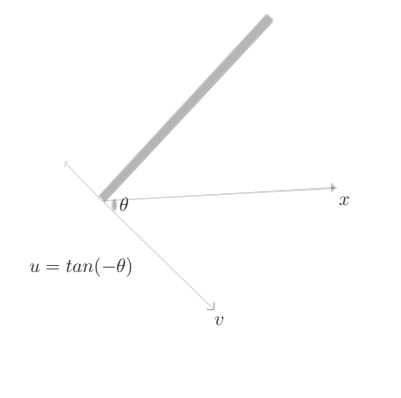
The natural dual slicing statement with the mass dimension was recently shown to be true by the author [13]. When dealing with the slicing question with a \(1\) separated set in \(\mathbb{R}^2\), it is natural to work with a width 1 tube \(t_{u,v}\) which is explicitly described as:
\[t_{u,v} =\begin{cases} \left\{(x,y) \in \mathbb{R}^2 \ \middle| \ -\frac 1u x + v \sqrt{ 1 + \frac 1{u^2}} < y \leq -\frac 1u x + (v+1) \sqrt{ 1 + \frac 1{u^2}} \right\}, u\neq 0.\\ \{(x,y)\in \mathbb{R}^2 | v< x\leq v+1 \}, u=0.\end{cases} \tag{2}\]
This is a tube of width 1. The line perpendicular to this tube and passing through the origin, has slope \(u\). Henceforth we call this line \(t_{\perp}\). The displacement of the point of intersection of the left edge of \(t_{u,v}\) with \(t_{\perp}\), along \(t_{\perp}\) is given by the coordinate \(v\) . For the special case of \(u=0\), we have vertical tubes. This is shown in the Figure 1.
In [13], for the mass dimension in our setting of \(1\) separated subsets in \(\mathbb{R}^{2}\), with a Tchebysheff and Fubini type argument the slicing statement was first shown to be true in an asymptotic sense, and then it was also shown to be true for Lebesgue almost every slice. One then specializes to sets \(A,B \subset \mathbb{N}\) and considers the dimension of the intersection of the broken line \(\{(x,y): y=\lfloor \tilde{u}x +\tilde{v} \rfloor, \tilde{u}>0 \}\) with the Cartesian product set \(A \times B\). This broken line is a tube with a vertical cross section of length 1, and thus, in general, the width of the tube is less than or equal to 1. Thus the slicing theorems of [13] follow for such tubes.
We state the main slicing result with the mass dimension that was obtained earlier in [13].
Theorem 1.2. Let \(E \subseteq \mathbb{R}^2\) be a \(1\) separated set. Then for all \(v \in \mathbb{R}\), for Lebesgue-a.e. \(u \in \mathbb{R}_+\), \[\overline{D}(E \cap t_{u,v}) \leq \text{max} (0, \overline{D}(E)-1).\]
As a corollary to this, we obtained the main slicing result stated below, upon integrating over the \(v\) coordinate.
Theorem 1.2. Let \(E \subseteq \mathbb{R}^2\) be a \(1\) separated set. Then in the Lebesgue sense, for almost every tube \(t_{u,v}\) of width \(1\), slope \(u\), and displacement \(v\) along the projecting line, we have that \(\overline{D}(E \cap t_{u,v}) \leq \text{max} (0, \overline{D}(E)-1)\).
In this paper we show that the corresponding results with the counting dimension are false. This is what one would expect, since the counting dimension of every slice can be high if there are boxes of points in every slice at very sparsely separated locations, with the number of points in each box growing to infinity. This can happen even if the actual set \(E\) has low counting dimension.
We state our results for the counting dimension below:
Theorem 1.3.
1. For any \(\epsilon>0, u_{0}\in \mathbb{R}\), there exists \(E \subseteq \mathbb{Z}^2\) , such that for all \(v \in (-\epsilon, \epsilon)\), \[\overline{D}(E \cap t_{u_0,v})=D(E \cap t_{u_0,v})= D(E)=\overline{D}(E)=1.\]
2. For any \(\epsilon>0, u_{0}\in \mathbb{R}\), there exists \(E \subseteq \mathbb{Z}^2\) , such that for all \(v \in (-\epsilon, \epsilon)\), \[D(E \cap t_{u_0,v})= D(E)=1, \overline{D}(E \cap t_{u_0,v})=\overline{D}(E)=0.\]
The more interesting case of the above Theorem 1.3 is to construct the set \(E\) that is meagre in terms of the mass dimension, in part (2) .
Next we state the main theorem of this paper,
Theorem 1.4. For any \(\epsilon>0, v_{0}\in \mathbb{R}\), there exists \(E \subseteq \mathbb{Z}^2\), such that for all \(u \in (-\epsilon, \epsilon)\), \[D(E \cap t_{u,v_0})= D(E)=1.\]
This shows the difference from the behavior of the mass dimension, where for any one-separated subset \(E\subset\mathbb{R}^2\), we have for any \(v\in \mathbb{R}\), for Lebesgue-a.e. \(u\in \mathbb{R}\), \(\overline{D}(E\cap t_{u,v})\leq \text{max}(\overline{D}(E)-1,0)\), which is the content of Theorem 9 in [13].
The same construction of Theorem 1.4, will provide the counterexample to the statement of the Marstrand slicing theorem with the counting dimension. We state this separately as a theorem.
Theorem 1.5. For any \(\epsilon>0\), there exists \(E \subseteq \mathbb{Z}^2\) , such that for all \((u,v) \in (-\epsilon, \epsilon)\times (-\epsilon,\epsilon)\), \[D(E \cap t_{u,v})= D(E)=1.\]
In other words, we can construct a set \(E\subset \mathbb{Z}^{2}\) such that the slices of \(E\) by the tubes parametrized by a positive Lebesgue measure set have exceptionally high counting dimension.
In fact, this construction of Theorem 1.5 immediately gives us the following result:
Theorem 1.6. There exists a set \(E \subseteq \mathbb{N}^2\), so that the set \(U\) of parameters \((u,v)\), with \(u,v\in \mathbb{R}\), so that \[D \big(E \cap t_{(u,v)} \big) = D(E)=1 .\] is such that \(\lim\limits_{x\to \infty} \frac{|U \cap [-x,x]^{2}|}{(2x)^{2}}>0\).
One compares this result with the corresponding result for the mass dimension, Theorem 6 in [13].
In the next section, as an illustration we begin with a standard example that shows that the slicing result is sharp with the mass dimension, where we have a set so that every slice in a cone has mass dimension \(\frac{1}{2}\) while the set so constructed has mass dimension \(\frac{3}{2}\). This is a set where every slice in the cone has counting dimension 1, while the set itself has a subsequence of grid of points where the number of points in each grid grows in a two dimension sense, to infinity, and hence is itself of counting dimension 2. After that we construct a set where we have a growth of points in a linear ’diagonal’ manner within the cone which reduces the counting dimension of the set to 1, while every slice in the cone still has counting dimension 1.
We also show that the proof of Theorem 1.6 essentially follows from the construction used in Theorem 1.5. This is the strongest slicing statement we can make with the counting dimension.
We remark that the analysis here again remains the same if in place of \(\mathbb{Z}^{2} \subset \mathbb{R}^{2}\), we considered the grid \(\delta\mathbb{Z}^{2}\) with separation \(\delta\), and considered tubes of width \(\delta\).
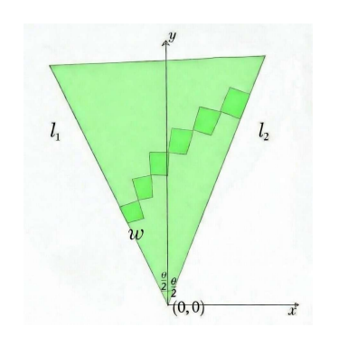
Throughout the rest of the paper, we use the term ‘box’ of points to mean a subset of the form \(T_{a_1,a_2,b_1,b_2}=\{(x,y)\in \mathbb{Z}^{2}: a_1\leq x\leq a_2, b_1\leq y\leq b_2 \}\) for some integers \(a_1\leq a_2, b_1\leq b_2\), or of the form \(\overline{T}_{r_1,r_2,\theta_1,\theta_2}\{re^{i\theta}\in \mathbb{Z}^2 : r_1 \leq r\leq r_2, \theta_1 \leq \theta\leq \theta_2 \}\) for any \(r_1\leq r_2, \theta_1\leq \theta_2\). We would also talk about boxes of points within a cone \(\mathscr{C}\), or a box of points within a tube \(t_{(u,v)}\) in which case it will be understood to mean \(T_{a_1,a_2,b_1,b_2}\cap \mathscr{C}, \overline{T}_{r_1,r_2,\theta_1,\theta_2}\cap \mathscr{C}\), or \(T_{a_1,a_2,b_1,b_2}\cap t_{(u,v)} , \overline{T}_{r_1,r_2,\theta_1,\theta_2}\cap t_{(u,v)}\) respectively. When talking about such boxes, we will not enumerate the set of values of \(a_1,a_2,b_1,b_2\) as above, and it should be understood from the context that we mean a box of this type. Also, in several places, we use the term ’level’ to indicate the collection of boxes of the set \(E\) within the cone \(C\), which are at approximately the same height from the origin (such as shown in Figure 2).
We construct the set that proves Theorem 1.3.
Proof of Theorem 1.3. (1) This example just consists of the set of the form \(\{(x,y\in \mathbb{Z}^{2}: -\epsilon/2 < x\leq \epsilon/2), y\geq 0\}\). Given any \(u_0\in \mathbb{R}\), one rotated this above set to get the desired set.
(2) Again, the set \(E\) is contained within the semi-infinite strip of width \(\epsilon\), \(S_\epsilon:= \{(x,y)\in \mathbb{Z}^2: – \epsilon/2 <x\leq \epsilon/2, y\geq 0 \}\). We place a box of points, \(B_1\), in \(S_\epsilon\cap \{(x,y):0\leq y\leq 1\}\). Define \(h_1:=1\). At the next stage, we place a box \(B_2\) in \(S_\epsilon\cap \{(x,y):e^{h_1}\leq y\leq e^{h_1}+2\}\). Inductively, for \(k\geq 2\), in the \(k'\)th step, we define \(h_k := e^{h_{k-1}}+k\), and put the box of points \(B_m\) in \(S_\epsilon\cap \{(x,y): h_m – m\leq y\leq h_m \}\).
It is clear that this is a set where, between heights \(h_{m} -m\) and \(h_{m}\) we have, for the purpose of the counting dimension, in effect a straight block of width \(w\) and length \(m\to \infty\) as \(m\to \infty\). It is clear that \(D(E)=1\). Moreover, every single tube with \(v\in V\) contains \(\sim m\) many points at the \(m\)’th level, and thus also of counting dimension exactly 1.
We clearly have \(h_{m}> \underbrace{e^{e^{… }}}_{m \ \text{times}}\) and till that height we have \(\epsilon(1+2+\dots+m)=c\epsilon m^2\) many points in \(E\). Thus clearly this set \(E\) has mass dimension 0. It’s similarly also clear that every width 1 tube with parameter \((u_{0},v)\), \(v\in (\epsilon/2,\epsilon/2)\), has mass dimension 0 because of the exponential separation between the different boxes of points used in the construction. ◻
Now we prove Theorem 1.41.
Proof of Theorem 1.4. In proving Theorem 1.4, it would be enough to construct the set \(E\) in the case of \(v_0 =0\). It is readily seen that the case of \(v_0 \neq 0\) is dealt with, with minor adjustments.
Without loss of generality, consider the cone \(\mathcal{C}\) with the vertex at the origin, and pointing up, symmetric about the y axis, and with total angle \(\theta\), and thus \(\epsilon=\tan \theta/2\). Call the set of tubes \(\mathcal{F}_\epsilon=\{t_{u,0}:- \epsilon\leq u\leq \epsilon\}\) . Call the left edge of the cone \(l_1\), and the right edge of the cone \(l_2\). Here, all tubes in \(\mathcal{F}_\epsilon\) have the coordinate \(v=0\), and we have an interval of \(u\) values of angular width \(\theta\).
We fix an initial length \(n_{1}=1\), and an initial height \(h_1\). Adjacent to \(l_1\), we put a box of width \(2\) and length \(n_{1}\),2 just above the arc at height \(h_{1}\). More precisely, this is the set \[\begin{aligned} E_{1,1}:= \left\{ re^{i\theta}\in \mathbb{Z}^2: h_1 \leq r\leq h_1 +n_1, -\tan^{-1} \epsilon\leq \theta\leq -\tan^{-1}\epsilon+\frac{2}{h_1} \right\}. \end{aligned} \tag{3}\]
This subtends the angle \((-\frac{\theta}{2},-\frac{\theta}{2}+\frac{2}{h_{1}})\) at the origin.
In the next step, we put a similar block of width \(2\) and length \(n_1\) just above the arc at height \(h_1 +n_1\), so this subtends the angle \(\left(-\frac{\theta}{2}+\frac{2}{h_{1}},-\frac{\theta}{2}+ \frac{2}{h_1}+ \frac{2}{h_1+n_1}\right)\) of width \(\frac{2}{h_1+n_1}\). In the \(k\)’th step, we put a block of width \(2\) at the height \(h_1 +(k-1)n_1\) so that it subtends the angle \(\left(-\frac{\theta}{2}+\sum\limits_{i=0}^{k-2} \frac{2}{h_{1}+i\cdot n_{1}},-\frac{\theta}{2}+\sum\limits_{i=0}^{k-1}\frac{2}{h_{1}+i\cdot n_1}\right)\) of width \(\frac{2}{h_1 +(k-1)\cdot n_1}\). Clearly the growth of the total angle is like that of the harmonic series, and eventually after some step \(K_1\) we reach the other end of the cone at the angle \(\theta/2\). In this process, the width of the last box adjacent to \(l_2\), at the height \(H_{1}:=h_1 +(K_1-1)n_1\) could be less than \(2\). These define the sets \(E_{l,1}\) for each \(1\leq l\leq K_1\), and thus the first level \(E_{1}\) of the set \(E\) is defined as the disjoint union: \[\begin{aligned} E_{1}:=\cup_{l=1}^{K_1} E_{l,1}. \end{aligned} \tag{4}\]
Consider the next height \(h_2:=e^{H_{1}}\), and \(n_{2}:=n_1 +1\) while the width \(2\) remains fixed. Now, the growth of points is here is similar to the growth in the first level, and we begin the growth again from the left edge \(l_1\) of the cone starting at the height \(h_{2}\). At the \(k\)’the stage in this level, we put a block of width \(2\), of length \(n_2\), at the height \(h_2 +(k-1)n_{2}\) which subtends the angle \(\left(-\frac{\theta}{2}+\sum\limits_{i=0}^{k-2}\frac{2}{h_2 +i\cdot n_{2}}, -\frac{\theta}{2}+\sum\limits_{i=0}^{k-1}\frac{2}{h_{2}+i\cdot n_{2}}\right)\) of width \(\frac{2}{h_{2}+(k-1)\cdot n_{2}}\). Again, after a finite number \(K_2\) of steps, we would hit the right edge \(l_2\) of the cone, where again at the last end, the width of the integer grid just above the height \(H_2:=h_2 +(K_{2}-1)n_2\) is less than or equal to \(2\). This defines the second level \(E_{2}\) of the set \(E\).
For each \(m\geq 3\), we inductively define \(h_{m}:=e^{H_{m-1}}\) and \(n_{m}:=n_{m-1}+1\) (Thus \(n_{m}=n_{1}+(m-1)\)) and thus have a growth of points beginning at the left edge \(l_1\) at height \(h_m\) and continuing on to height \(H_{m}\) at the last \(K_{m}\)’th step of the iteration in this \(m\)’th level, where this last box of the integer grid is put adjacent to the right edge \(l_2\) of the cone \(\mathcal{C}\).
Thus the set \(E\) can be written as, \[\begin{aligned} E=\cup_{m=1}^{\infty} E_{j}=\cup_{m=1}^{\infty}\cup_{l=1}^{K_m} E_{l,m}. \end{aligned} \tag{5}\]
Now for any tube \(t\in \mathcal{F}_\epsilon\) , we have \(D(t\cap E)=1\); since for each of these tubes, at the \(m\)’th level, there is a box within the tube where the number of points is between \(n_{m}\) and \(2n_{m}\). Further, by construction, these boxes are exponentially separated.
We also have \(D(E)=1\), since at each particular \(m\)’th level, we have a set of boxes, each of width \(2(1+o(1))\), each of length \(n_1 + (m-1)\), the \(k\)’th box lying just above and to the right of the \((k-1)\)’th box. If we had a square of length \(K_{m}\cdot (n_{1}+(m-1))\) intersect the set \(E\) at this appropriate height, then for the purpose of the counting dimension this is equivalent to having a vertical straight line of length \(\approx K_{m}\cdot(n_1 +(m-1))\) within this square. As \(m\to \infty\), the lengths of these boxes go to infinity, and we conclude that \(D(E)=1\). ◻
Note the difference between the cases in Theorems 1.3 and 1.4. In the case of Theorem 1.3, the construction gives a tube of some fixed width in which we case exponentially separated blocks of growing length. For the purpose of the counting and mass dimension, these tubes have fixed a-priori widths and thus are of counting dimension \(1\). In the construction of Theorem 1.3 however, the constructed set \(E\) lies within a cone. In this case, if we mimmick the proof of Theorem 1.3 and put a box of points that covered an entire annular region \(\mathcal{C}\cap \{re^{i\theta}\in \mathbb{Z}^2 :r_1\leq r\leq r_2\}\) for any given \(r_1,r_2\), then for the purpose of the counting dimension, such sets are clearly sets of counting dimension \(2\). The subtlety in our construction in Theorem 1.4 thus involves a diagonally growing sequence at each level within the cube \(C\).
Now with this same set \(E\), we can further show that the natural Marstrand slicing statement with the counting dimension is false.
Proof of Theorem 1.5.The construction follows from that in the previous theorem, by considering the same set \(E\), withing the cone \(\mathcal{C}\). This set of tubes is denoted by \(\mathcal{F}_1:=\{(u,v): -\epsilon\leq v\leq \epsilon, -\epsilon \leq u \leq \epsilon \}\), with the same \(\epsilon\) as considered in Theorem 1.4.
Consider any tube \(t\in \mathcal{F}_1\). Consider any sequence of points \(p_k =(x_k,y_k)\in E\cap t\), with \(y_k\) belonging to the \(k\)’th level, and take \(k\to \infty\). For each \(k\), consider the line \(l_k\) joining \(p_k\) to the origin. It is obvious that as \(k\to \infty\), the angle \(\theta_k\) between the right (or left) edge of the tube \(t\) and the line \(p_k\) goes to \(0\) in the limit of \(k\to \infty\). It is then easy to see that as \(k\to \infty\), the number of points in \(t\) at the \(k\)’th level tends to \(Cn_k\), for a universal constant \(C\).
We conclude that the set \(E\) is such that every \(t \in\mathcal{F}_1\) has \(D(t)=1\) . The difference from Theorem 1.4 here is that these tubes parameterized by the \(u\neq 0\) parameters intersect the boxes of \(E\) ‘obliquely’, while still having counting dimension 1. ◻
Now the proof of Theorem 1.6 is immediate with the same set \(E\).
Proof of Theorem 1.6. Again consider the same set \(E\), within the cone \(\mathcal{C}\). Consider all the tubes \(t_{(u,v)}\) whose right edges are lines that intersect the set \(E\) with slopes in the range \(( \cot \theta/2,\infty)\), and thus the slope \(m(t_{\perp})\) of the line \(t_{\perp}\) being \(0\leq m(t_{\perp})\leq \tan (\theta/2)\) ( The same is true of tubes whose right edges have negative slopes in the range \((-\tan (\theta/2),0)\)). By the argument of Theorem 1.5 these tubes have counting dimension exactly 1.
This set of tubes is given by \[\left\{(u,v)\in \Big( (0,\tan (\theta/2))\times (0,\infty )\Big) \cup \Big((-\tan (\theta/2),0)\cup (-\infty,0)\Big) \right\},\](recall the parametrization shown in 1). All these tubes have an infinite intersection with the cone \(\mathcal{C}\) as well as the set \(E\) and the intersection of each such tube \(t_{(u,v)}\) with \(E\) is such that \(D(E\cap t_{(u,v)})=1=D(E)\). Thus with \(S=\Big( (0,\tan (\theta/2))\times (0,\infty )\cup (-\tan (\theta/2),0)\cup (-\infty,0)\) we have \(\lim_{x\to \infty} \frac{ |S| \cap [-x,x]^{2}}{(2x)^{2}} >0\) and so the weak asymptotic form of the slicing theorem is also false for the counting dimension. ◻
1. While we show that a positive Lebesgue measure set of tubes of width 1 have exceptionally large dimension, the question of constructing sets such that a set of broken lines \(\{(x,y): y=\lfloor ux+v \rfloor \}\) with positive Lebesgue measure in the parameter space \((\tilde{u},\tilde{v})\), all have exceptionally large counting dimension, is not resolved here. The broken lines are sets that have vertical cross section 1, but the actual width is smaller than unity, and so there is no guarantee that a large number of broken lines have exceptionally high dimension, let alone a set of broken lines parametrized by a positive Lebesgue measure set in the \((u,v)\) space. Such a question will likely require a much finer study of the intersection patterns of tubes of arbitrary small width with the integer grid \(\mathbb{Z}^{2}\subset \mathbb{R}^{2}\).
2. While we have constructed our sets in \(\mathbb{R}^2\), there should be a natural way to extend these results in higher dimensions, and while the construction in Theorem 1.3 would be extended to higher dimension in an obvious way, we would likely have to be a bit more careful in constructing the cones in dimensions 3 and higher while proving the results analogous to Theorem 1.4.
3. We aim to study the question of sets of exceptions to the Marstrand type slicing statement of [13] for the mass dimension, as well as the Marstrand type projection theorems proved in [7, 9] and the dimensions of the parameter set of tubes that violate the inequality in the Lebesgue a.e. sense. This will likely involve ergodic and diophantine approximation techniques, and draw on the literature for the study of exceptional sets for the classical Marstrand projection and slicing theorems.
The author is thankful to Stephen Montgomery-Smith for a careful reading of the manuscript and suggesting improvements. The author also thanks Daniel Glasscock for introducing the author to the slicing problem in the integer lattice grid in \(\mathbb{R}^{2}\).
The author certifies that he has no known affiliations or involvement in any organization or entity with any financial interest, or non-financial interest in the subject matter or materials discussed in this manuscript.