
Let \(G = (V, E)\) be a graph with vertex set \(V\) of order \(n = |V|\), and edge set \(E\), of size \(m = |E|\). Given an edge \(uv \in E\), we say that vertices \(u\) and \(v\) are adjacent and that they are neighbors. The (open) neighborhood of a vertex \(u \in V\) is the set \(N(u) = \{v : uv \in E\}\) of neighbors of \(u\). The degree of a vertex \(u \in V\) is \(deg(u) = |N(u)|\), the number of neighbors of \(u\). A vertex of degree zero, that is, a vertex having no neighbors, is called an isolated vertex. The maximum degree of a vertex in a graph \(G\) is denoted by \(\Delta(G)\). The closed neighborhood of a vertex \(u\) is the set \(N[u] = N(u) \cup \{u\}\).
Given a set \(S \subset V\) of vertices in a graph \(G = (V, E)\), the subgraph of \(G\) induced by \(S\) is the graph \(G[S] = (S, E(S))\), with vertex set \(S\) and an edge \(uv \in E(S)\) if and only if \(u,v \in S\) and \(uv \in E(G)\).
A path \(P_n = (V, E)\) of order \(n\) and size \(n-1\) is a graph with vertex set \(V = \{v_1, v_2, \ldots, v_n\}\) and edge set \(E = \{v_i v_{i+1}, 1 \le i \le n-1\}\). We say that \(P_n\) is path of length \(n-1\).
A cycle \(C_n\) of order \(n \ge 3\) and size \(n\) is a graph of the form \(C_n = P_n \cup \{v_1 v_n\}\), consisting of a path \(P_n\) with the added edge between \(v_1\) and \(v_n\).
A complete graph \(K_n = ( V, E)\) of order \(n\) is a graph in which for every \(u,v \in V\), \(uv \in E\). With this definition we could say that an isolated vertex in a graph \(G\) is an induced subgraph of the form \(K_1\), and similarly an isolated edge is an induced subgraph of the form \(K_2\), consisting of two adjacent vertices both of degree \(1\).
A set \(S \subset V\) of vertices is independent if no two vertices in \(S\) are adjacent, or equivalently, if the subgraph \(G[S]\) induced by \(S\) consists of a set of isolated vertices. A set \(S\) is called \(1\)-dependent if the subgraph \(G[S]\) induced by \(S\) has maximum degree one, or equivalently, if the subgraph induced by \(S\) consists of isolated vertices \(K_1\)s and isolated edges \(K_2\)s.
The Cartesian product of two graphs \(G_{1} = (V_{1}, E_{1})\) and \(G_{2} = (V_{2}, E_{2})\) is the graph \(G_{1} \Box G_{2} = (V_{1} \times V_{2}, E_{12})\), such that two vertices \((u_{1},u_{2})\) and \((v_{1}, v_{2})\) are adjacent in \(E_{12}\) if and only if either \(u_{1} = v_{1}\) and \(u_{2}v_{2} \in E_{2}\) or \(u_{2} = v_{2}\) and \(u_{1}v_{1} \in E_{1}\).
A (rectangular) grid graph \(G_{m,n}\) is a Cartesian product of the form \(P_{m} \Box P_{n}\), for integers \(m,n \geq1\), where \(P_{m}\) and \(P_{n}\) denote paths of length \(m-1\) and \(n-1\), respectively.
A set \(S \subset V\) of vertices in a graph \(G = (V, E)\) is a dominating set if every vertex in \(w \in V – S\) is adjacent to at least one vertex in \(S\), that is, \(|N(w) \cap S| \ge 1\). The domination number \(\gamma(G)\) of a graph \(G\) equals the minimum cardinality of a dominating set \(S\) in \(G\)
A dominating set \(S\) is a perfect dominating set if for every vertex \(w \in V-S\), \(|N(w) \cap S| = 1\), that is, every vertex in \(V – S\) has exactly one neighbor in \(S\).
A perfect dominating set is an efficient dominating set or a \(1\)-efficient dominating set if for every vertex \(v \in S\), \(|N[v] \cap S| = 1\), that is, \(S\) is an independent set. Thus, an efficient dominating set \(S\) is a set that is both an independent set and a perfect dominating set.
Not every graph \(G\) has an efficient dominating set. Two simple examples are the cycles \(C_{4}\) and \(C_{5}\), although it is easy to see that all cycles \(C_{3k}\), for \(k \geq1\), have an efficient dominating set. We say that graphs having an efficient dominating set are efficient.
A perfect dominating set \(S\) is a total efficient dominating set or \(2\)-efficient dominating set if for every vertex \(v \in S\), \(|N(v) \cap S| = 1\), that is, every vertex in \(S\) has exactly one neighbor in \(S\). Thus, a total efficient dominating set \(S\) is a set that is both a \(1\)-dependent set and a perfect dominating set.
Not every graph \(G\) has a total efficient dominating set. A simple example is the cycle \(C_{5}\), although it is easy to see that all cycles \(C_{4k}\), for \(k \geq1\), have a total efficient dominating set. We say that graphs having a total efficient dominating set are total efficient.
A perfect dominating set \(S\) is a 1,2-efficient dominating set if for every vertex \(v \in S\), \(1 \le |N[v] \cap S| \le 2\), that is, every vertex in \(S\) has either no neighbors in \(S\) or exactly one neighbor in \(S\), or equivalently, if \(S\) is a 1-dependent set. Thus, a 1,2-efficient dominating set \(S\) is a set that is both a \(1\)-dependent set and a perfect dominating set.
Efficient domination is of considerable importance in many real-world applications, cf. any of the following books [14, 15, 16, 17, 18]. Efficient dominating sets have minimum cardinality of all dominating sets in a graph, but even more, they dominate the vertices of a graph with no redundancy or overlap, in that no vertex in \(V-S\) is dominated two or more times. And thus, they provide domination at absolute minimum cost. In coding theory, efficient dominating sets are called perfect codes, which means that they correspond to single-error-correcting codes. This means that every vertex, or code word, is either a member of a dominating set, or is adjacent to a unique member of the dominating set, which represents the corrected code word.
Many papers have been published on the domination numbers of grid graphs, too numerous to be cited here. Over the years many authors [4, 5, 6, 11, 12, 13, 21, 23] have developed techniques for either computing \(\gamma(G_{m,n})\) exactly or establishing lower or upper bounds for \(\gamma(G_{m,n})\). An historical overview of developments is the following:
[1983] Jacobson and Kinch [19] determined \(\gamma(G_{m,n})\) for \(1 \leq m \leq 4\) and all \(n\).
[1989] Hare [12] determined several domination numbers of \(G_{m,n}\) for \(7 \leq m \leq 11\).
[1992] In his PhD thesis, Chang [2] conjectured that for all \(m,n \geq 16\), \[\gamma(G_{m,n}) = \left \lfloor \frac{(m+2)(n+2)}{5} \right \rfloor – 4.\]
[1993] Chang and Clark [3] determined \(\gamma(G_{m,n})\) for \(m = 5, 6\) and all \(n\).
[1998] Fisher [8] presented a method for computing \(\gamma(G_{m,n})\) that was described in the 2001 PhD thesis of Spalding [24], who determined the values of \(\gamma(G_{m,n})\) for \(m \leq 19\) and all \(n\).
[2001] Mao [22] proved that the domination number of \(G_{m,n}\) is no more than\([(m+2)(n+2)/5] – 4\), for sufficiently large \(m\) and \(n\).
[2011] Alanko, Crevals, Insopoussu, Ø̈stergärd, and Petterson [1] used dynamic programming to extend these results to \(m \leq 29\) and all \(n\). Of particular interest in this paper is the presentation of minimum dominating sets for all square grid graphs \(G_{n,n}\), for \(1 \leq n \leq 29\).
[2011] Chang’s conjecture was proved true by Goncalves, Pinlou, Rao and Thomasse [10], as follows.
Theorem 3.1 (Goncalves, Pinlou, Rao, Thomasse).For all \(1 \leq m \leq n\):
\[\begin{aligned} \gamma(P_1 \Box P_n) =& \gamma(P_n) =\left \lceil \frac{n}{3} \right \rceil = \left \lfloor \frac{n+2}{3} \right \rfloor,\\ \gamma(P_2 \Box P_n) =& \left \lfloor \frac{n+2}{2} \right \rfloor = \left \lceil \frac{n+1}{2} \right \rceil,\\ \gamma(P_3 \Box P_n) =& \left \lfloor \frac{3n+4}{4} \right \rfloor = n – \left \lfloor \frac{n – 1}{4} \right \rfloor,\\ \gamma(P_4 \Box P_n) =& \left\{ \begin{array}{cl} n + 1 & \mbox{if $n = 5, 6, 9$}; \\ n & \mbox{otherwise}, \end{array} \right.\\ \gamma(P_5 \Box P_n) =& \left\{ \begin{array}{cl} \left \lfloor \dfrac{6n+6}{5} \right \rfloor & \mbox{if $n = 7$}; \\ [3mm] \left \lfloor \dfrac{6n+8}{5} \right \rfloor & \mbox{otherwise}, \end{array} \right.\\ \gamma(P_6 \Box P_n) =& \left\{ \begin{array}{cl} \left \lfloor \dfrac{10n+10}{7} \right \rfloor & \mbox{if $n \equiv 1 \pmod{7}$}; \\ [3mm] \left \lfloor \dfrac{10n+12}{7} \right \rfloor & \mbox{otherwise}, \end{array} \right.\\ \gamma(P_7 \Box P_n) =& \left \lfloor \dfrac{5n+3}{3} \right \rfloor,\\ \gamma(P_8 \Box P_n) =& \left \lfloor \dfrac{15n+14}{8} \right \rfloor,\\ \gamma(P_9 \Box P_n) =& \left \lfloor \dfrac{23n+20}{11} \right \rfloor,\\ \gamma(P_{10} \Box P_n) =& \left\{ \begin{array}{cl} \left \lfloor \dfrac{30n+37}{13} \right \rfloor & \mbox{if $n \neq 13, 16, n \equiv 0,3 \pmod{13}$}; \\[3mm] \left \lfloor \dfrac{30n+24}{13} \right \rfloor & \mbox{otherwise}, \end{array} \right.\\ \gamma(P_{11} \Box P_n) =& \left\{ \begin{array}{cl} \left \lfloor \dfrac{38n+21}{15} \right \rfloor & \mbox{if $n = 11, 18, 20, 22, 33$}; \\ [3mm] \left \lfloor \dfrac{38n+36}{15} \right \rfloor & \mbox{otherwise}, \end{array} \right.\\ \gamma(P_{12} \Box P_n) =& \left \lfloor \frac{80n+66}{29} \right \rfloor,\\ \gamma(P_{13} \Box P_n) =& \left\{ \begin{array}{cl} \left \lfloor \dfrac{98n+111}{33} \right \rfloor & \mbox{if $n \not\equiv 14, 15, 17, 20 \pmod{33}$}; \\ [3mm] \left \lfloor \dfrac{98n+78}{33} \right \rfloor & \mbox{otherwise}, \end{array} \right.\\ \gamma(P_{14} \Box P_n) =& \left\{ \begin{array}{cl} \left \lfloor \dfrac{35n+40}{11} \right \rfloor & \mbox{if $n \equiv 18 \pmod{22}$}; \\ [3mm] \left \lfloor \dfrac{35n+29}{11} \right \rfloor & \mbox{otherwise}, \end{array} \right.\\ \gamma(P_{15} \Box P_n) =& \left\{ \begin{array}{cl} \left \lfloor \dfrac{44n+27}{13} \right \rfloor & \mbox{if $n \equiv 5 \pmod{26}$}; \\ [3mm] \left \lfloor \dfrac{44n+40}{13} \right \rfloor & \mbox{otherwise}. \end{array} \right.\\ \gamma(P_m \Box P_n) =& \left \lfloor \frac{(m+2)(n+2)}{5} \right \rfloor – 4, \mbox{ for all $m, n \geq 16$}. \end{aligned}\]
The total domination numbers of grid graphs has also received a fair amount of attention, although no complete set of formulas, as in the preceding theorem by Goncalves et al., for the total domination numbers of \(G_{m,n}\) exists, for all \(m\) and \(n\). We refer the interested reader to the 20-page Chapter 17 in the 2023 book by Haynes, Hedetniemi and Henning [18].
In 1990 Livingston and Stout [20] completely determined which grid graphs are efficient, and there are indeed very few.
Theorem 4.1. [20] A grid graph \(G_{m,n}\), for \(m,n \ge2\), has an efficient domination set if and only if either (i) \(m = n = 4\), or (ii) \(m = 2\) and \(n = 2k+1\), for \(k \ge1\).
Figure 1 illustrates the unique (up to isomorphism) efficient dominating set of the \(4 \times 4\) grid graph \(G_{4,4}\).
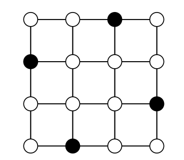
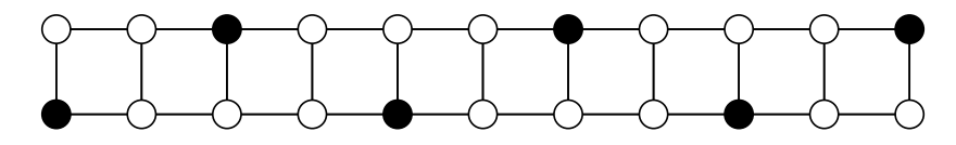
Figure 2 illustrates the unique, up to isomorphism, efficient dominating set of the \(2 \times11\) grid graph \(G_{2,11}\).
The question of which grid graphs are total efficient was considered by Gavlas and Schultz for \(m = 1\) in 2002 [9], and then by Cowen, Hechler, Kennedy and Steinberg in 2007 [7], who proved the following.
Theorem 4.2 ([7]).For all \(m,n > 1\), if both \(m\) and \(n\) are odd, then \(G_{m,n}\) is not total efficient.
The determination of all total efficient grid graphs was settled by Klostermeyer and Goldwasser in 2006 [25].
Theorem 4.3 ([25]).For all \(m,n \ge 1\),
(i) \(G_{1,n}\) is total efficient if and only if \(n \not\equiv 1\mod{4}\).
(ii) for \(m,n > 1\), \(G_{m,n}\) is total efficient if and only if \(m\) is even and \(n\mod{(m+1)} \in \{1, m-2, m\}\).
Figure 3 illustrates a total efficient dominating set of the \(6 \times 11\) grid graph \(G_{6,11}\).
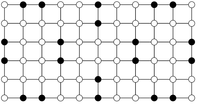
Notice, however, that Figure 3 illustrates much more than this. For example, the leftmost four columns illustrate a total efficient dominating set of \(G_{6,4}\); the first six columns illustrate a total efficient dominating set of \(G_{6,6}\); and the first four columns restricted to the top four rows illustrate a total efficient dominating set of \(G_{4,4}\).
Notice as well in Figure 3 that in a total efficient set in a grid graph, and as we will see in a 1,2-efficient set in a grid graph, every vertex in the set is distance three from of at least one other vertex in the set, either what is called a knight’s move away or a horizontal or vertical path of length three away.
In this section we introduce the study of the \(1,2\)-efficiency of \(m \times n\) grid graphs \(G_{m,n}\).
Since Livingston and Stout have shown that all paths \(P_n \simeq G_{1,n}\) are efficient, they are by definition \(1\)-efficient and therefore, 1,2-efficient as well.
Theorem 5.1 ([20]). All \(1 \times n\) grid graphs \(G_{1,n} \simeq P_n\) are 1,2-efficient.
The Klostermeyer-Goldwasser characterization of total efficient grid graphs suffices to show that all \(2 \times n\) grid graphs are 1,2-efficient, since they are all total, or 2-efficient.
Theorem 5.2 ([25]).All \(2 \times n\) grid graphs \(G_{2,n}\) are 1,2-efficient.
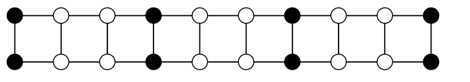
Figure 4 illustrates a total efficient dominating set of the \(2 \times 10\) grid graph \(G_{2,10}\), which is, therefore, a 1,2-efficient dominating set. This pattern clearly repeats indefinitely. Notice in this figure that the first two columns show that \(G_{2,2}\) is 1,2-efficient; columns 3,4,5 show that \(G_{2,3}\) is 1,2-efficient; the first four columns and the first five columns show that \(G_{2,4}\) and \(G_{2,5}\) are 1,2-efficient, respectively; columns 3 through 8 show that \(G_{2,6}\) is 1,2-efficient; etc..
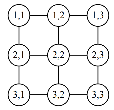
Proposition 5.3. The grid graph \(G_{3,3}\) is not 1,2-efficient.
Proof. Assume that the vertices in \(G_{3,3}\) are labeled as shown in Figure 5.
Assume that \(G_{3,3}\) has a 1,2-efficient dominating set \(S\). Consider the three vertices \((1,1), (2,1), (3,1)\) in the first column. They cannot all be in \(S\), else vertex \((2,1)\) has two neighbors in \(S\). Similarly, if no vertex in the first column is in \(S\), then in order that all three are dominated, all three vertices in the second column would have to be in \(S\), but in this case vertex \((2,2)\) would have two neighbors in \(S\); a contradiction.
Thus, by symmetry, there are only two cases for the first column.
Case 1. One vertex in the first column is in \(S\).
Case 1a. \((1,1) \in S\), but \((2,1), (3,1) \notin S\). In this case in order to dominate \((3,1)\), \((3,2) \in S\). But in this case, \((1,2)\) cannot be in \(S\) else \((2,2)\) is dominated twice; \((2,3)\) cannot be in \(S\) else \((2,2)\) is dominated twice; and \((1,3)\) cannot be in \(S\) else \((1,2)\) is dominated twice. This means that vertex \((1,3)\) cannot be in \(S\) or dominated by exactly one vertex in \(S\).
Case 1b. \((2,1) \in S\), but \((1,1), (3,1) \notin S\).
Case 1b.1. \((2,2) \notin S\). In this case \((1,2)\) cannot be in \(S\) else \((1,1)\) is dominated twice; \((3,2)\) cannot be in \(S\) else \((3,1)\) is dominated twice. Thus, in order to dominate \((1,2)\), vertex \((1,3)\) must be in \(S\). But now \((3,3)\) cannot either be in \(S\) (else \((2,3)\) is dominated twice), or be dominated by a vertex in \(S\), since \((3,2)\) can’t be in \(S\) (else \((3,1)\) is dominated twice), and \((2,3)\) can’t be in \(S\) (else \((2,2)\) is dominated twice).
Case 1b.2. \((2,1), (2,2) \in S\). But in this case, vertex \((1,3)\) cannot be dominated, since it cannot be in \(S\), else \((1,2)\) is dominated twice, and it cannot be dominated by a vertex in \(S\) since neither \((1,2)\) nor \((2,3)\) can be in \(S\).
Case 2. Two vertices in the first column are in \(S\). Clearly \((1,1), (3,1) \in S\) but \((2,1) \notin S\) is not possible else \((2,1)\) is dominated twice. Thus, without loss of generality, assume that \((1,1), (2,1) \in S\), but \((3,1) \notin S\). In this case vertex \((1,2)\) cannot be in \(S\) else \((1,1)\) has two neighbors in \(S\); vertex \((2,2)\) cannot be in \(S\) else \((2,1)\) has two neighbors in \(S\); vertex \((1,3)\) cannot be in \(S\) else \((1,2)\) has two neighbors in \(S\), and vertex \((2,3)\) cannot be in \(S\) else \((2,2)\) has two neighbors in \(S\). Thus, vertex \((1,3)\) cannot be in \(S\) or dominated by a vertex in \(S\).
From the above cases it follows that \(G_{3,3}\) does not have a 1,2-efficient dominating set. ◻
Proposition 5.4. The grid graph \(G_{3,5}\) is not 1,2-efficient.
Proof. Assume that the grid graph \(G_{3,5}\) has a 1,2-efficient dominating set \(S\). As in the proof of Proposition 5.3 we can assume that \(S\) contains either one or two vertices from the first column.
Case 1. \((1,1) \in S\), \((2,1), (3,1) \notin S\) (cf. Figure 6). The only way to dominate \((3,1)\) is by having \((3,2) \in S\). But once \((3,2) \in S\) then neither \((1,2)\) nor \((2,2)\) nor \((2,3)\) can be in \(S\), and therefore, since \((1,3)\) can’t be in \(S\), \((1,4)\) must be in \(S\) in order to dominate \((1,3)\). But now, the only way to dominate \((2,3)\) is for \((2,4)\) to be in \(S\). But if \((1,1), (3,2), (1,4), (2,4) \in S\), then vertex \((3,5)\) cannot be in \(S\) or dominated by \(S\).
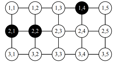
Case 2. \((2,1) \in S\), \((1,1), (3,1) \notin S\) (cf. Figure 7). In this case, if \((2,2) \notin S\) then \((1,3)\) must be in \(S\) in order to dominate \((1,2)\) and \((3,3)\) must be in \(S\) in order to dominate \((3,2)\). But then \((2,3)\) has two neighbors in \(S\). Thus, we can assume that \((2,2) \in S\). In this case \((1,4)\) must be in \(S\) in order to dominate \((1,3)\), while \((3,4)\) must be in \(S\) in order to dominate \((3,3)\). But in this case \((2,4)\) has two neighbors in \(S\).
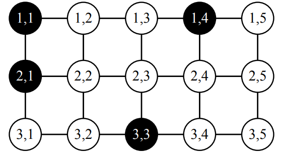
Case 3. \((1,1), (2,1) \in S\), \((3,1) \notin S\) (cf. Figure 8). In this case, \((3,3)\) must be in \(S\) in order to dominate \((3,2)\), which then implies that \((1,4)\) must be in \(S\) in order to dominate \((1,3)\). But in this case vertex \((3,5)\) cannot be in \(S\) nor dominated by a vertex in \(S\).
From the above cases it follows that \(G_{3,5}\) does not have a 1,2-efficient dominating set.
Theorem 5.5. Other than \(G_{3,3}\) and \(G_{3,5}\), all \(3 \times n\) grid graphs \(G_{3,n}\) are 1,2-efficient.
Proof. The following three figures suffice to prove that other than \(G_{3,3}\) and \(G_{3,5}\), all \(3 \times n\) grid graphs \(G_{3,n}\) are 1,2-efficient. Notice in Figure 9 that the pattern of black vertices in the leftmost four columns can be repeated indefinitely to the right, showing that all grid graphs of the form \(G_{3,4k}\) are 1,2-efficient.
In addition, you can aways remove the rightmost two columns and create a 1,2-efficient grid of the general form \(G_{3,4k-2}\) or \(G_{3,4k+2}\).
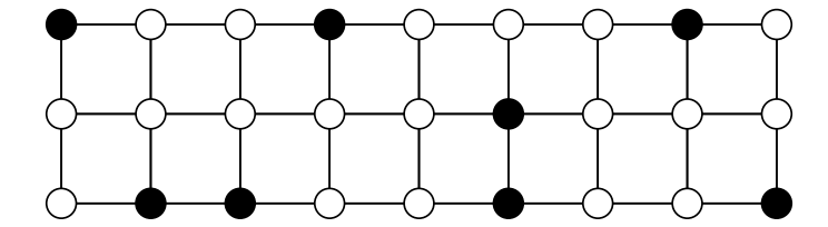
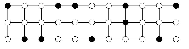
Figure 10 shows how to add, to the right of any repeating first four columns, an additional 5 columns (columns 5 through 9), in effect creating a 1,2-efficient grid of the form \(G_{3,4k+1}\), while Figure 11 shows how to attach an additional seven columns (columns 5 through 11), creating a 1,2-efficient grid of the form \(G_{3,4k+3}\). ◻
Theorem 5.6. All \(4 \times n\) grid graphs \(G_{4,n}\), for \(n \ge 1\), are 1,2-efficient.
Proof. Previous results above have shown that \(G_{4,1} \simeq G_{1,4}\), \(G_{4,2} \simeq G_{2,4}\) and \(G_{4,3} \simeq G_{3,4}\) are \(1,2\)-efficient. Figure 12 suffices to prove that \(G_{4,n}\) is 1,2-efficient for all \(n \ge 4\). Notice that the first five columns can repeat indefinitely, showing that grid graphs of the form \(G_{4,5k}\) are 1,2-efficient, for all \(k \ge 1\). Adding a column identical to column 6 in Figure 12 to the right of a repeating first five \(5\) columns of Figure 12 shows that grid graphs of the form \(G_{4,5k+1}\) are 1,2-efficient.
Adding two columns identical to columns 7 and 8 of Figure 12 to the right of a repeating \(5\) columns shows that grid graphs of the form \(G_{4,5k+2}\) are 1,2-efficient.
Adding three columns identical to columns 6, 7 and 8 of Figure 12 to the right of a repeating \(5\) columns shows that grid graphs of the form \(G_{4,5k+3}\) are 1,2-efficient.
And finally, adding four columns identical to columns 7, 8, 9 and 10 of Figure 12 to the right of a repeating \(5\) columns shows that grid graphs of the form \(G_{4,5k+4}\) are 1,2-efficient. ◻
We have previously showed that \(G_{3,5} \simeq G_{5,3}\) is not 1,2-efficient.
Proposition 5.7. The grid graph \(G_{5,9}\) is not \(1,2\)-efficient.
Proof. This result was obtained by an exhaustive computer search, which analyzed some 1,299,393,735 cases in 25 minutes of machine time. This program builds a \(5 \times 9\) grid row-by-row, representing the vertices in one row in a proposed 1,2-efficient dominating set in binary, 1 representing a chosen vertex, 0 representing an unchosen vertex. Rows containing either a 101 or 111 are eliminated. Similarly, proposed solutions containing either a 101 or 111 in a column are eliminated. When the prerequisite number of 5 rows and 9 columns have been constructed, then a simple check is made to see that every unchosen vertex has exactly one chosen neighbor, and every chosen vertex has no more than one chosen neighbor. ◻
Theorem 5.8. Other than \(G_{5,3}\) and \(G_{5,9}\), all grid graphs \(G_{5,n}\) are 1,2-efficient.
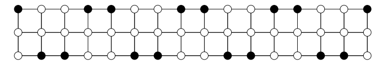
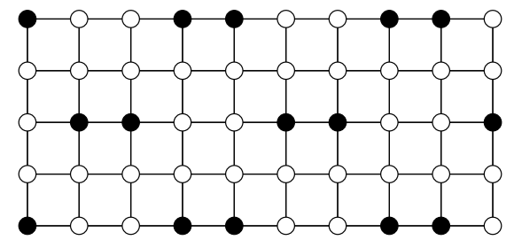
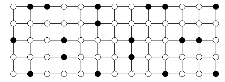
Proof. Figure 13 suffices to show that all grid graphs of the form \(G_{5,2k}\) are 1,2-efficient. Notice in this figure that the first two columns show that \(G_{5,2}\) is 1,2-efficient. The same applies to the first four columns \(G_{5,4}\), the first six columns \(G_{5,6}\), the first eight columns \(G_{5,8}\), and all ten columns \(G_{5,10}\). By simply repeating this pattern of adding two or four columns one can show that all grid graphs \(G_{5,2k}\), for \(k \ge 1\), are 1,2-efficient.
In order to show that for all \(k \ge 5\), all grid graphs of the form \(G_{5,2k+1}\) are 1,2-efficient, consider first Figure 14 and Figure 15 which show that \(G_{5,5}\) and \(G_{5,7}\) are 1,2-efficient.
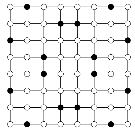
For \(5 \times (2k+1)\), for \(k \ge 5\) consider Figure 16, which shows that \(G_{5,11}\) is 1,2-efficient.
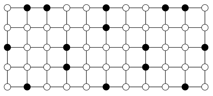
If we attach a copy of the first two columns of Figure 16 to the right end of Figure 16 we get the 1,2-efficient \(G_{5,13}\) in Figure 16.
If you notice the pattern of vertices in the rightmost four columns of Figure 17 you will see that this is a repeatable pattern, and thus the two extensions shown in Figure 16 and Figure 17 can be repeated indefinitely, showing that for all \(k \ge 5\), \(G_{5,2k+1}\) is 1,2-efficient.
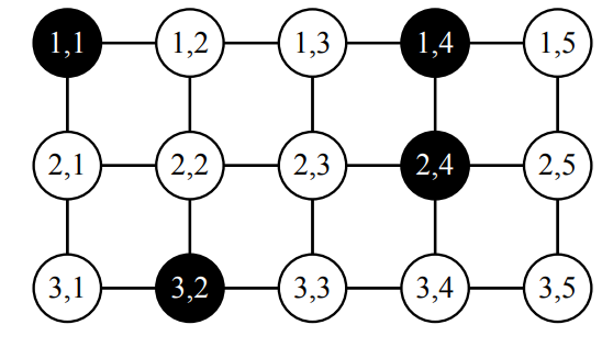
Theorem 5.9. All \(6 \times n\) grid graphs \(G_{6,n}\) for \(n \in \{7k, 7k+1, 7k+2, 7k+4, 7k+6\}\) are 1,2-efficient.
Proof. Consider Figure 18. Since this pattern repeats indefinitely, in blocks of seven columns, we know that \(G_{6,7k+1}\), \(G_{6,7k+4}\) (attach a copy of columns 2,3,4 to the right of this repeating pattern), and \(G_{6,7k+6}\) (attached a copy of columns 2,3,4,5,6 to the right of this repeating pattern) are all 1,2-efficient, in fact they are all total, or 2-efficient, for all \(k \ge 1\), as proved by Klostermeyer and Goldwasser in Theorem 4.3.
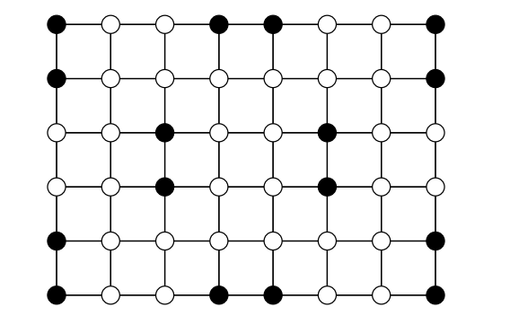
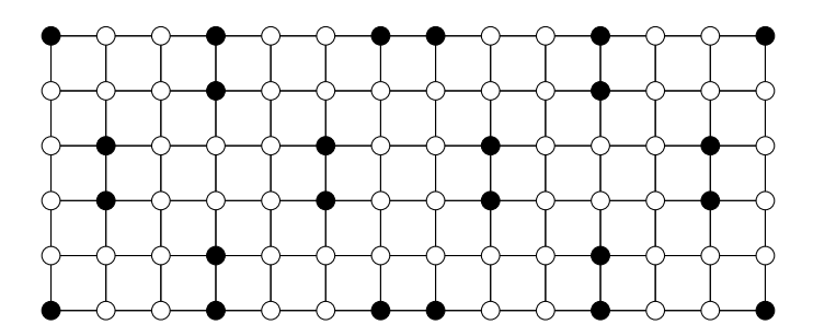
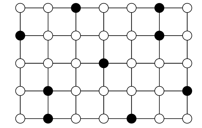
Figure 19 shows that all grid graphs of the form \(G_{6,7k}\) are 1,2-efficient by repeating the first seven columns indefinitely. Furthermore, adding a copy of the first two columns of this \(G_{6,14}\) pattern to the right of this repeating pattern of seven columns shows that all grids graphs of the form \(G_{6,7k+2}\) are also 1,2-efficient. Thus, all grids of the form \(G_{6,7k}\), \(G_{6,7k+1}\), \(G_{6,7k+2}\), \(G_{6,7k+4}\), and \(G_{6,7k+6}\) are 1,2-efficient. ◻
Problem 5.10(Open problem).This leaves one to settle the 1,2-efficiency of \(G_{6,7k+3}\) and \(G_{6,7k+5}\).
We have yet to determine, for arbitrary \(m\) and \(n\), which grid graphs \(G_{m,n}\) are 1,2-efficient. In this section we prove that all even-by-odd grid graphs \(_{2m,2n+1}\) and all even-by-even grid graphs of the form \(G_{4m,4n}\) are 1,2-efficient.
Recall Theorem 4.3(ii) that asserts that all 2-by-odd grid graphs are 1-efficient, as shown in Figure 2. Consider therefore Figure 20, in which every consecutive pair of rows, proceeding from top to bottom, is a 2-by-odd 1-efficient set. This is sufficient to show that every even-by-odd grid graph is 1,2-efficient.
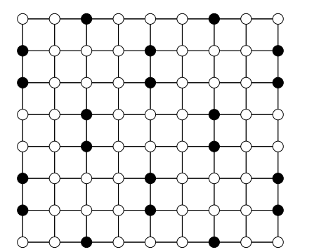
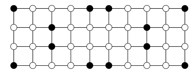
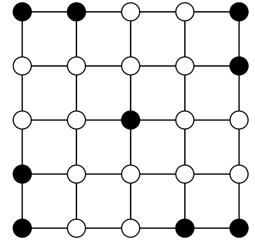
We start with the following \(2\)-dimensional replication of the simple \(4\)-by-\(4\) \(1\)-efficient grid in Figure 21, which shows that grids of the form \(G_{4m,4n}\) are 1,2-efficient, since a new row of 4×4 cells can always be added below this figure and similarly, a new column of 4×4 cells can always be added to the right of this figure.
Problem 6.1 (Open Problem).Are all even-by even grid graphs \(G_{2m,2n}\) 1,2-efficient?
Using a computer program, we have determined, for various small values of \(m,n \le 20\), the number of non-isomorphic 1,2-efficient sets a grid graph \(G_{m,n}\) has, cf. Figure 22. These repeating patterns of numbers suggest many conjectures.
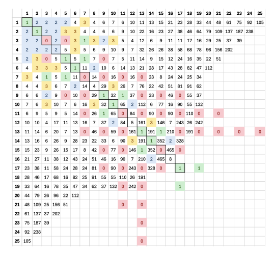
Notice, first of all, that in every case so far known in which \(G_{m,n}\) is not 1,2-efficient, both \(m\) and \(n\) are odd.
Notice as well, that those grids having a unique (up to isomorphism) 1,2-efficient set, are so far the following: \(G_{1,1}\), \(G_{2,2}\), \(G_{3,7}\), \(G_{5,5}\), \(G_{5,7}\), \(G_{9,9}\), \(G_{9,11}\), \(G_{10,10}\), \(G_{10,11}\), \(G_{13,13}\), \(G_{13,15}\), and \(G_{14,14}\).
From the data in Figure 22 one is tempted to make the following conjectures.
Conjecture 7.1. For all \(k \ge 1\), \(G_{2^k,2^k}\) has \(2^{k-1}\) non-isomorphic 1,2-efficient dominating sets.
Conjecture 7.2. For all \(m,n \ge 1\), \(G_{2m,2n}\) is 1,2-efficient.
Conjecture 7.3. For all \(m,n \ge 1\), \(G_{m,n}\) is 1,2-efficient if either \(m\) or \(n\) is even.
Conjecture 7.4. For all odd \(m = 3 + 4k\), \(k \ge 0\), \(G_{m,n}\) is 1,2-efficient if and only if \(n \notin \{3+4k+2(j-1) : 1 \le j \le 2(k+1)\}\).
Conjecture 7.5. For all odd \(m = 5+ 4k\), \(k \ge 0\), \(G_{m,n}\) is 1,2-efficient if and only if \(n \notin \{5+4k +2(j-1) : 1 \le j \le 2(k+1) – 1\}\).
Conjecture 7.6. For all \(k \ge 1\), \(G_{4k+1,4k+1}\) is 1,2-efficient.
Conjecture 7.7. For all \(m \ge 2\), \(G_{2m,2m+2}\) and \(G_{2m,2m-2}\) have, up to isomorphism, exactly three 1,2-efficient sets.
Conjecture 7.8. For all \(m = 4k+1\), for \(k \ge 0\), \(G_{m,m}\) has a unique 1,2-efficient set.
Conjecture 7.9. For all \(m = 4k+2\), for \(k \ge 0\), \(G_{m,m}\) has a unique 1,2-efficient set.
Can you characterize the grid graphs that are not 1,2-efficient? For example, are the 1,2-inefficient grid graphs only odd-by-odd \(G_{2m+1,2n+1}\), where \(n \le f(m)\), where \(f(m)\) is some function of \(m\)? Based on our data so far, it appears that for \((2m+1,2n+1) \in \{(3,5), (5,9), (7,13), (9,17), (11,21),(13,25) \}\), \(G_{2m+1,4m+1}\) is not 1,2-efficient, but if \(2n+1 \ge 4m+1\), then \(G_{2m+1,2n+1}\) is 1,2-efficient.
What can you say about 1,2-efficient Cartesian products?
What can you say about 1,2-efficient cylinders, i.e. Cartesian products of the form \(C_m \Box P_n\) or \(P_m \Box C_n\)?
What can you say about 1,2-efficient toroidal graphs, i.e. Cartesian products of the form \(C_m \Box C_n\)?
Can you characterize 1,2-efficient trees?
Can you show that the following decision problem is NP-complete?
1,2-EFFICIENT
INSTANCE: Graph \(G = (V, E)\)
QUESTION: Is \(G\) 1,2-efficient?
What are formulas for the 1,2-efficient domination numbers of \(m \times n\) grid graphs, for various values of \(m\)?
What can you say about grid graphs which have a unique 1,2-efficient dominating set?
Some grid graphs can have 1,2-efficient dominating sets of different cardinalities. If so, then there are two parameters \(\gamma_{1,2\varepsilon}(G)\) and \(\Gamma_{1,2\varepsilon}(G)\), the minimum and maximum cardinalities of a 1,2-efficient set in a graph \(G\). What can you say about these two parameters?
How do \(\gamma_{1,2}(G)\) and \(\gamma_{1,2\varepsilon}(G)\) compare, for 1,2-efficient graphs?