
The concept of graphs was introduced in 1736 by Euler [3] and has since become a fundamental tool in various fields. A graph, indicated as \(G\), is defined as a pair of ordered components \(G=(V,E)\), where \(V\) represents the collection of vertices and \(E\) represents the collection of edges attached to the vertices. A graph with directed edges is called a Digraph, which allows for representing asymmetrical relationships between nodes. In contrast, undirected graphs only depict symmetrical relationships.
The concept of connectedness has importance in the field of graph theory. If a graph is considered \(connected\) then there exists at least one path between any two arbitrary vertices; otherwise, it is \(disconnected\). A digraph is classified as \(strongly\) \(connected\) if there exists a path from any vertex \(x\) to any vertex \(y\), as well as from \(y\) to \(x\). Conversely, a digraph is termed \(weakly \ connected\) if there is a path between any two vertices regardless of the edge direction. The Degree of a vertex in a graph refers to the number of edges associated with it. For digraphs, the indegree of a vertex \(a\) represents the count of edges in the form \(x\rightarrow a\) while the outdegree signifies the number of edges in the form \(a\rightarrow y\). In a graph, the distance between two vertices \(x\) and \(y\) is denoted by \(d(x, y)\) and signifies the shortest possible length of the path traversed between them. It should be emphasised that in non-commutative rings, the distance between \(x\) and \(y\) may not be symmetric, meaning that the distance between \(x\) and \(y\) may not be equal to the distance between \(y\) and \(x\). The diameter of a graph \(G\), represented as \(diam(G)\), is the maximum distance between any two vertices. Additionally, the girth of a graph, denoted as girth, represents the length of the smallest cycle present in a graph.
The notation \(End(G)\) represents the set of \(group\) \(endomorphisms\) of a group \(G\). This set forms a ring when given the operation of map addition, defined as \((f + g)(x) = f(x) + g(x)\) \(\forall\) elements \(x\) \(\in\) \(G\). The operation of map composition is defined as the product of two endomorphisms \(f\) and \(g\), denoted as \((fg)(x) = f(g(x))\) \(\forall\) elements \(x\) \(\in\) \(G\). Let \(A\) be a group such that \(A = \bigoplus_{i=1}^{n} A_i\), the endomorphism ring is isomorphic to the ring of \(n \times n\) matrices \([\alpha_{ji}]\), where \(\alpha_{ji}\) belongs to \(Hom(A_i, A_j)\), employing ordinary matrix addition and multiplication [4].
To facilitate a deeper understanding of ring endomorphisms, we shall examine two illustrative examples that elucidate the concept. Let \(R=\mathbb{Z}\), the ring of integers, and consider the map \(\Phi_1:\mathbb{Z} \rightarrow \mathbb{Z}\) defined by \(\Phi_1(x)=2x\) \(\forall\) \(x \in \mathbb{Z}\). We see that \(\Phi\) is a ring endomorphism. Again, let us consider the ring \(R=\mathbb{Z}/6\mathbb{Z}\), the integers modulo 6. Define the map \(\Phi_2:\mathbb{Z}/6\mathbb{Z} \rightarrow \mathbb{Z}/6\mathbb{Z}\) by \(\Phi_2(x)=3x \ mod \ 6\) where \(x \in \mathbb{Z}/6\mathbb{Z}\). We clearly see that \(\Phi_2\) is a ring endomorphism.
Graph theory and ring theory are two branches of mathematics that have found profound applications in various areas of study. One intriguing connection between these fields arises from the exploration of \(zero \ divisor \ graphs\) associated with rings. These graphs provide insights into the underlying algebraic structure and properties of the corresponding rings. Beck in [2] demonstrated the correlation between ring theory and graph theory. Beck established the definition of an undirected graph \(G(R)\) with the set of vertices \(V(R)\) for a given commutative ring \(R\). The graph which consists of vertices \(x\) and \(y\) are connected if and only if their product \(xy\) is equal to zero. It is worth noting that \(G(R)\) is a simple graph, with no self-loops, excluding the consideration of \(nilpotent \ elements\) in the ring. Furthermore, every vertex in \(G(R)\) is connected to the zero vertex, ensuring its connectivity with a diameter of at most \(2\). Beck’s work primarily focused on graph coloring.
A zero divisor in a ring \(R\) is a nonzero element \(a \in R\) such that there exists a nonzero element \(b \in R\) where \(a.b=0\). Zero divisors cannot exist in fields but are common in rings.
Example 1.1. Zero Divisors in \(\mathbb{Z}/10\mathbb{Z}\). Consider the ring of integers modulo 10, \(\mathbb{Z}/10\mathbb{Z}\). The elements of this ring are \(\{0,1,2,3,4,5,6,7,8,9\}\).
\(\bullet\) Let \(a=2\) and \(b=5\). Then \(a.b=2.5=10 \equiv 0 (mod 10)\).
\(\bullet\) Neither \(a=2\) nor \(b=5\) is zero in \(\mathbb{Z}/10\mathbb{Z}\), but their product is zero. Hence, both \(a=2\) and \(b=5\) are zero divisors.
Anderson and Livingston [1] modified this definition of \(zero \ divisor \ graph\) introduced by Beck. Instead of considering all elements of the ring \(R\) as the vertex set, they specifically focused on the zero divisors of \(R\).
A zero-divisor graph of a commutative ring \(R\) is a graph where the vertices are the non-zero zero divisors of \(R\), and two vertices are connected by an edge if their product is zero in \(R\).
Example 1.2. Zero Divisor Graph of \(\mathbb{Z}/6\mathbb{Z}\)
\(\bullet\) Elements of \(\mathbb{Z}/6\mathbb{Z}\): The elements are \(\{0,1,2,3,4,5\}\).
\(\bullet\) Zero Divisors in \(\mathbb{Z}/6\mathbb{Z}\): An element \(a \in R\) is a zero divisor if there exists a non-zero \(b\in R\) such that \(a.b=0 \ mod \ 6\). For \(R=\mathbb{Z}/6\mathbb{Z}\): \(2.3=6 \equiv 0(mod \ 6)\), \(3.2=6 \equiv 0(mod \ 6)\), \(4.3=12 \equiv 0(mod 6)\). Thus, the non-zero zero divisors are: \(Z^{\ast}(R)={2,3,4}\).
\(\bullet\) Constructing the Graph:
Vertices: \(Z^{\ast}(R)={2,3,4}\).
Edges: \((2,3)\) because \(2.3=0(mod \ 6)\), \((3,4)\) because \(3.4=0(mod \ 6)\).
Graph Representation: The graph is a simple graph with vertices \(2,3,4\) and edges connecting \(2\) to \(3\) and \(3\) to \(4\).
Definition 1.3. Let \(Z(R)^{\ast}\) denote the set of non-zero zero divisors for a ring \(R\). The zero divisor graph \(\Gamma(R)\) is a graph whose vertices are the non-zero divisors of the ring \(R\), that is, \(Z(R)^{\ast}\). Two distinct vertices \(x\) and \(y\) are connected by an edge if and only if their product \(xy\) is equal to zero.
Anderson and Livingston demonstrated that \(\Gamma(R)\) is a connected graph with a diameter of at most \(3\).
Redmond expanded the concept and definition of the \(zero \ divisor \ graph\) for commutative rings to \(zero \ divisor \ graph\) for non-commutative rings [5].
Definition 1.4. The directed zero divisor graph \(\Gamma(R)\) is defined for a non-commutative ring \(R\) with the vertex set \(Z(R)^{*}\)in such a way that an edge from vertex \(x\) to vertex \(y\) exists in \(\Gamma(R)\) if and only if the product of \(x\) and \(y\) is equal to zero.
Let \(R\) be a ring, left zero divisors and right zero divisors are elements \(a \in R\) that meet the conditions \(ax = 0\) and \(ya = 0\), respectively, where \(x\) and \(y\) are non-zero elements. The left zero divisors of \(R\) are indicated as \(\mathcal{Z}_L(R)\), whereas the right zero divisors are denoted as \(\mathcal{Z}_R(R)\). In the paper by Redmond (refer [5]), it was shown that the connectedness of \(\Gamma(R)\) is dependent upon the equality of \(\mathcal{Z}_L(R)\) and \(\mathcal{Z}_R(R)\). Furthermore, if \(\Gamma(R)\) is indeed \(connected\) then its diameter is at most \(3\). For more study on \(zero \ divisor \ graph\), one can refer [8, 7, 9, 6].
We delve into the \(zero \ divisor \ graph\) of the endomorphism ring of the direct product of groups in this research work. Endomorphism rings capture the set of all \(group\) \(homomorphisms\) from a group to itself, forming a ring under the operation of function composition. By examining the \(zero \ divisor \ graph\) of the endomorphism ring of a direct product of groups, we aim to uncover significant characteristics and investigate their implications. The findings of this research have the potential to contribute to both graph theory and ring theory. Understanding the \(zero \ divisor \ graph\) of the endomorphism ring of the direct product of groups will shed light on the algebraic properties of these rings and provide a deeper understanding of their structural characteristics. Moreover, the insights gained from this study can have implications in areas such as group theory, algebraic topology, and cryptography.
Through this research, we aim to bridge the gap between graph theory and ring theory, unraveling the intriguing connections between these fields and contributing to the broader understanding of algebraic structures in mathematics.
In this section, first we discuss the general structure of \(zero \ divisor \ graph\) of \(End(\mathbb{Z}_2 \times \mathbb{Z}_{2p})\), for odd prime \(p\). We know that \[\begin{aligned} End(\mathbb{Z}_2 \times \mathbb{Z}_{2p}) \cong& \begin{bmatrix} Hom(\mathbb{Z}_2,\mathbb{Z}_2) & Hom(\mathbb{Z}_{2p},\mathbb{Z}_2) \\ Hom(\mathbb{Z}_2,\mathbb{Z}_{2p}) & Hom(\mathbb{Z}_{2p},\mathbb{Z}_{2p}) \end{bmatrix}\\ =& \left\{ \begin{bmatrix} a & b \\ c & d \end{bmatrix} \mid a=0,1, \ b=0,1, \ c=0,p, \ d=0,1,\dots,(p-1) \right \}. \end{aligned}\]
Here we are interested in finding number of zero divisors, maximum and minimum vertex degree, whether indegree is equal to outdegree for every element. Let \(\begin{bmatrix} a & b \\ c & d \end{bmatrix}\) be an arbitrary element of \(End(\mathbb{Z}_2 \times \mathbb{Z}_{2p})\). We find conditions on \(a,b,c\) and \(d\) for which \(\begin{bmatrix} a & b \\ c & d \end{bmatrix}\) is a left and right zero divisor of any element. Throughout the paper, \((x,2p)\) represent g.c.d of \(x\) and \(2p\).
| Element | \(Z_{R}\) | \(Z_{L}\) |
|---|---|---|
| \(\begin{bmatrix} 0 & 1 \\ 0 & 0 \end{bmatrix}\) | \(a=0,1, \ b=0,1, \ c=0 d=0,2,\dots,p-1\) | \(a=0, \ b=0,1, \ c=0, d=0,1,\dots,p-1\) |
| \(\begin{bmatrix} 1 & 0 \\ 0 & 0 \end{bmatrix}\) | \(a=0, \ b=0, \ c=0,p d=0,1,\dots,p-1\) | \(a=0, \ b=0,1, \ c=0, d=0,1,\dots,p-1\) |
| \(\begin{bmatrix} 0 & 0 \\ p & 0 \end{bmatrix}\) | \(a=0, \ b=0, \
c=0,p \) \( d=0,1,\dots,p-1\) |
\(a=0,1, \ b=0,
\ c=0,p \) \( d=0,2,\dots,p-1\) |
| \(\begin{bmatrix} 1 & 0 \\ 0 & 0 \end{bmatrix}\) | \(a=0, \ b=0, \
c=0,p \) \( d=0,1,\dots,p-1\) |
\(a=0, \ b=0,1,
\ c=0 \) \( d=0,1,\dots,p-1\) |
| \(\begin{bmatrix} 0& 0 \\ 0 & x \end{bmatrix} \mid (x,2p)=1\) | \(a=0,1, \
b=0,1, \ c=0 \) \( d=0\) |
\(a=0,1, \ b=0,
\ c=0,p \) \( d=0\) |
| \(\begin{bmatrix} 0 & 0 \\ 0 & x \end{bmatrix} \mid (x,2p)=2\) | \(a=0, \ b=0,1,
\ c=0,p \) \( d=0,p\) |
\(a=0,1, \
b=0,1, \ c=0,p \) \( d=0,p\) |
| \(\begin{bmatrix} 0 & 0 \\ 0 & p \end{bmatrix}\) | \(a=0,1, \
b=0,1, \ c=0 \) \( d=0,2,\dots,p-1\) |
\(a=0,1, \ b=0,
\ c=0,p \) \( d=0,2,\dots,p-1\) |
| \(\begin{bmatrix} 1 & 1 \\ 0 & 0 \end{bmatrix}\) | \((a,c)=(0,0)(1,p) \) \( (b,d)=(0,0)(0,2)\dots(0,p-1)(1,1)(1,3)\dots (1,p-2)\) |
\(a=0, \ b=0,1,
\ c=0 \) \( d=0,1,\dots,p-1\) |
| \(\begin{bmatrix} 1 & 0 \\ p & 0 \end{bmatrix}\) | \(a=0, \ b=0, \
c=0,p \) \( d=0,1,\dots,p-1\) |
\((a,b)=(0,0)(1,1),\
(c,d)=(0,0)(0,2)\dots(0,p-1)\) \((1,1)(1,3)\dots (1,p-2)\) |
| \(\begin{bmatrix} 0 & 1 \\ p & 0 \end{bmatrix}\) | \(a=0, \ b=0, \
c=0 \) \( d=0,2,\dots,p-1\) |
\(a=0, \ b=0, \
c=0 \) \( d=0,2,\dots,p-1\) |
| \(\begin{bmatrix} 0 & 1 \\ 0 & x \end{bmatrix} \mid (x,2p)=1\) | \(a=0,1, \
b=0,1, \ c=0 \) \( d=0\) |
\((a,b)=(0,0)(1,1) \) \( (c,d)=(0,0)(p,p)\) |
| \(\begin{bmatrix} 0 & 1 \\ 0 & x \end{bmatrix} \mid (x,2p)=2\) | \(a=0,1, \
b=0,1, \ c=0 \) \( d=0\) |
\((a,b)=(0,0)(0,1) \) \( (c,d)=(0,0)(0,p)\) |
| \(\begin{bmatrix} 0 & 1 \\ 0 & p \end{bmatrix}\) | \(a=0,1, \
b=0,1, \ c=0 \) \( d=0,2,\dots,2p-2)\) |
\((a,b)=(0,0)(1,1),\ (c,d)=(0,0)(0,2)\dots
(0,2p-2)\) \((p,1)(p,3)\dots (p,2p-1)\) |
| \(\begin{bmatrix} 0 & 0 \\ p & x \end{bmatrix} \mid (x,2p)=1\) | \((a,c)=(0,0)(1,p) \) \( (b,d)=(0,0)(1,p)\) |
\(a=0,1, \ b=0,
\ c=0,p \) \( d=0\) |
| \(\begin{bmatrix} 0 & 0 \\ p & x \end{bmatrix} \mid (x,2p)=2\) | \((a,c)=(0,0)(0,p) \) \( (b,d)=(0,0)(0,p)\) |
\(a=0,1, \ b=0,
\ c=0,p \) \( d=0\) |
| \(\begin{bmatrix} 0 & 0 \\ p & p \end{bmatrix}\) | \((a,c)=(0,0)(1,p),\
(b,d)=(0,0)(0,2)\dots(0,2p-2)\) \( (1,1)(1,3)\dots (1,2p-1)\) |
\(a=0,1, \ b=0,
\ c=0,p \) \( d=0,2,\dots,p-1\) |
| \(\begin{bmatrix} 1 & 0 \\ 0 & x \end{bmatrix} \mid (x,2p)=2\) | \(a=0, \ b=0, \
c=0,p \) \( d=0,p\) |
\(a=0, \ b=0,1,
\ c=0 \) \( d=0,p\) |
| \(\begin{bmatrix} 1 & 0 \\ 0 & p \end{bmatrix}\) | \(a=0, \ b=0, \
c=0 \) \( d=0,2,\dots,p-1\) |
\(a=0, \ b=0, \
c=0 \) \( d=0,2,\dots,p-1\) |
| \(\begin{bmatrix} 1 & 1 \\ p & 0 \end{bmatrix}\) | \(a=0, \ b=0, \
c=0 \) \( d=0,2,\dots,p-1\) |
\(a=0, \ b=0, \
c=0 \) \( d=0,2,\dots,p-1\) |
| \(\begin{bmatrix} 1 & 0 \\ p & x \end{bmatrix} \mid (x,2p)=2\) | \(a=0, \ b=0, \
c=0,p \) \( d=0,p\) |
\((a,b)=(0,0)(1,1) \) \( (c,d)=(0,0)(p,p)\) |
| \(\begin{bmatrix} 1 & 0 \\ p & p \end{bmatrix}\) | \(a=0, \ b=0, \
c=0 \) \( d=0,2,\dots,p-1\) |
\(a=0, \ b=0, \
c=0 \) \( d=0,2,\dots,p-1\) |
| \(\begin{bmatrix} 0 & 1 \\ p & p \end{bmatrix}\) | \(a=0, \ b=0, \
c=0 \) \( d=0,2,\dots,2p-2\) |
\(a=0, \ b=0, \
c=0 \) \( d=0,2,\dots,2p-2\) |
| \(\begin{bmatrix} 1 & 1 \\ 0 & x \end{bmatrix} \mid (x,2p)=2\) | \((a,c)=(0,0)(1,p) \) \( (b,d)=(0,0)(1,p)\) |
\(a=0, \ b=0,1 \
c=0 \) \( d=0,p\) |
| \(\begin{bmatrix} 1 & 1 \\ 0 & p \end{bmatrix}\) | \(a=0, \ b=0, \
c=0 \) \( d=0,2,\dots,2p-2\) |
\(a=0, \ b=0, \
c=0 \) \( d=0,2,\dots,2p-2\) |
| \(\begin{bmatrix} 1 & 1 \\ p & x \end{bmatrix} \mid (x,2p)=1\) | \((a,c)=(0,0)(1,p) \) \( (b,d)=(0,0)(1,p)\) |
\((a,b)=(0,0)(1,1) \) \( (c,d)=(0,0)(p,p)\) |
| \(\begin{bmatrix} 1 & 1 \\ p & p \end{bmatrix}\) | \((a,c)=(0,0)(1,p),\
(b,d)=(0,0)(0,2)\dots(0,2p-2)\) \( (1,1)(1,3)\dots (1,2p-1)\) |
\((a,b)=(0,0)(1,1),\
(c,d)=(0,0)(0,2)\dots(0,2p-2)\) \( (1,1)(1,3)\dots (1,2p-1)\) |
Remaining elements \(\begin{bmatrix} 1 & 0 \\ 0 & x \end{bmatrix} \mid (x,2p)=1,\ \begin{bmatrix} 1 & 0 \\ p & x \end{bmatrix} \mid (x,2p)=1,\ \begin{bmatrix} 1 & 1 \\ 0 & x \end{bmatrix} \mid (x,2p)=1,\ \begin{bmatrix} 0 & 1 \\ p & x \end{bmatrix} \mid (x,2p)=1,\ \begin{bmatrix} 0 & 1 \\ p & x \end{bmatrix} \mid (x,2p)=2 \mbox{ and } \begin{bmatrix} 1 & 1 \\ p & x \end{bmatrix} \mid (x,2p)=1\) are not zero divisors. So, number of zero divisors including zero element are \[16p-6(p-1) = 10p + 6 .\]
We also observe that the only possible degrees are \(0,4,16,p\) and \(4p\). So we get the following result:
Cojecture 2.1. Minimum and maximum vertex degree of \(End(\mathbb{Z}_2 \times \mathbb{Z}_{2p})\) is:
(1) Maximum = 4p and Minimum = 4, p \(>\) 3.
(2) Maximum = 12 and Minimum = 3, p = 3.
Our most important observation is that \(\mid Z_{L}(R) \mid= \mid Z_{R}(R) \mid\) i.e., indegree is equal to outdegree for every element of \(End(\mathbb{Z}_2 \times \mathbb{Z}_{2p})\). We found other rings like \(End(\mathbb{Z}_p \times \mathbb{Z}_p)\) and \(End(\mathbb{Z}_p \times \mathbb{Z}_{2p})\) with the same property but this does not holds true for arbitary ring for which we give the following counter example:
Example 2.2. Consider the ring \(End(\mathbb{Z}_2 \times \mathbb{Z}_8)\). Let \(\begin{bmatrix} a & b \\ c & d \end{bmatrix}\) be any arbitary element. Then we have \[\begin{aligned} \begin{bmatrix} 0 & 1 \\ 0 & 0 \end{bmatrix} \begin{bmatrix} a & b \\ c & d \end{bmatrix} &=& \begin{bmatrix} c & d \\ 0 & 0 \end{bmatrix} = \begin{bmatrix} 0 & 0 \\ 0 & 0 \end{bmatrix} \mbox{ if } a=0,1,\ b=0,1, \ c=0,4,\ d=0,2,4,6 \\ \begin{bmatrix} a & b \\ c & d \end{bmatrix} \begin{bmatrix} 0 & 1 \\ 0 & 0 \end{bmatrix} &=& \begin{bmatrix} 0 & a \\ 0 & c \end{bmatrix} = \begin{bmatrix} 0 & 0 \\ 0 & 0 \end{bmatrix} \mbox{ if } a=0,\ b=0,1, \ c=0,\ d=0,1,2,3,4,5,6. \\ \end{aligned}\]
As we can see that number of right zero divisor of \(\begin{bmatrix} 0 & 1 \\ 0 & 0 \end{bmatrix} = 32\) but number of left zero divisor are 16.
In similar way, we studied \(zero \ divisor \ graph\) of ring \(End(\mathbb{Z}_2 \times \mathbb{Z}_{2^2p})\) and \(End(\mathbb{Z}_2 \times \mathbb{Z}_{2^3p})\) and came up with following result for ring \(End(\mathbb{Z}_2 \times \mathbb{Z}_{2^yp})\):
Conjecture 2.3. Number of zero divisors in the ring \(End(\mathbb{Z}_2 \times \mathbb{Z}_{2^yp})\) are \(2^{y+1}(3p+1)\).
Proof. We know that \(End(\mathbb{Z}_2 \times \mathbb{Z}_{2^yp}) \cong \begin{bmatrix} Hom(\mathbb{Z}_2,\mathbb{Z}_2) & Hom(\mathbb{Z}_{2^yp},\mathbb{Z}_2) \\ Hom(\mathbb{Z}_2,\mathbb{Z}_{2^yp}) & Hom(\mathbb{Z}_{2^yp},\mathbb{Z}_{2^yp}) \end{bmatrix}\). So, total number of elements are \(2 \times 2 \times 2 \times 2^{y}p = 2^{y+3}p\). Out of these, the elements of the form \(\begin{bmatrix} 1 & 0 \\ 0 & x \end{bmatrix}, \begin{bmatrix} 1 & 0 \\ 2^{y-1}p & x \end{bmatrix}, \begin{bmatrix} 1 & 1 \\ 0 & x \end{bmatrix}\) and \(\begin{bmatrix} 1 & 1 \\ 2^{y-1}p & x \end{bmatrix}\) where \((x,2^{y}p)=1\) are the only elements with no non zero zero divisor. Also number of elements coprime to \(2^{y}p\) are \(2^{y-1}(p-1)\). Hence, number of zero divisors are: \[\begin{aligned} 2^{y+3}p – 4[2^{y-1}(p-1)] =& 2^{y+1}(4p-p+1) \\ =& 2^{y+1}(3p+1). \end{aligned}\] ◻
So far, we have established and provided a rigorous proof for the conjecture, which proposes that the total number of zero divisors in the ring \(End(\mathbb{Z}_2 \times \mathbb{Z}_{2^y p})\) is given by the expression \(2^{y+1}(3p+1)\). This result not only confirms the validity of the conjecture but also offers a precise count of the zero divisors, thereby contributing to a deeper understanding of the algebraic structure of \(End(\mathbb{Z}_2 \times \mathbb{Z}_{2^y p})\).
Following this, we turn our attention to the next phase, which concerns a new conjecture. In this conjecture, the focus shifts from counting zero divisors to exploring the graphical representation associated with \(End(\mathbb{Z}_2 \times \mathbb{Z}_{2^y p})\). Specifically, we aim to determine the lower and upper bounds of the vertex degrees in the corresponding graph, with particular emphasis on how these bounds vary as the parameter \(p\) changes. Such bounds not only offer insights into the connectivity properties of the graph but also serve as essential tools for understanding the interplay between algebraic features of the ring and the combinatorial characteristics of its associated graph.
Conjecture 2.4. Minimum and maximum vertex degree of \(End(\mathbb{Z}_2 \times \mathbb{Z}_{2^y p})\) is:
(1) Maximum = \(2^{y+3}p\) and Minimum = 4, p \(>\) 3.
(2) Maximum = \(3(2^{y+3})\) and Minimum = 3, p = 3.
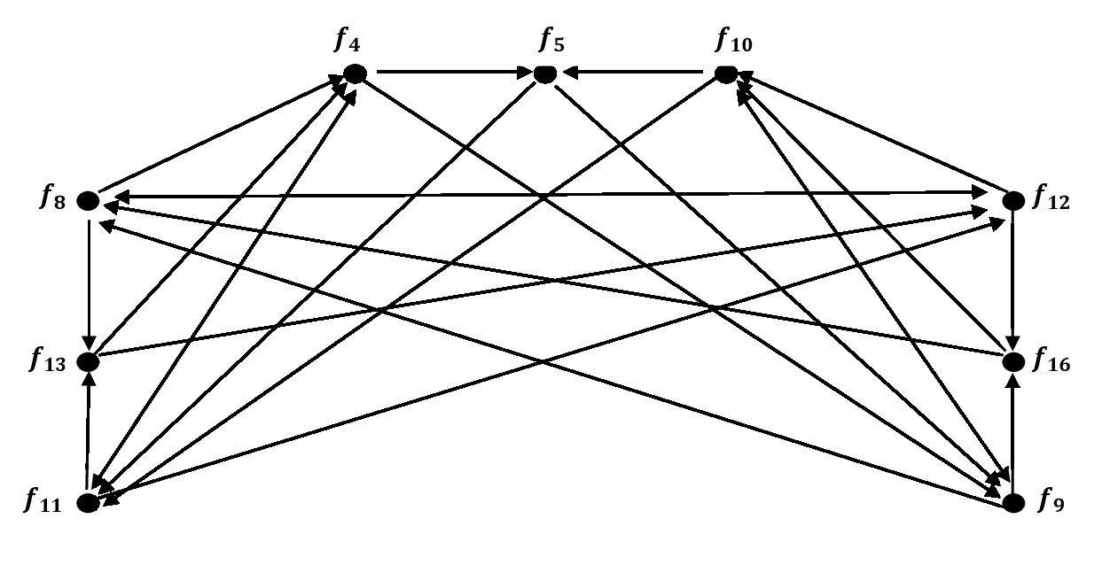
From the Figure 1, it is observant that the Zero divisor graph of \(End(\mathbb{Z_2} \times \mathbb{Z_2})\) is directed and after studying various examples of zero divisor graph of \(End(\mathbb{Z}_p \times \mathbb{Z}_p)\), it is established that the minimum distance between any two distinct vertices is 2.
Proposition 2.5. The minimum distance of the zero divisor graph of the ring \(Mat_n(R)\) is 2 for all domains \(R\) and \(n>1\).
Proof. (1) Let us begin by assuming that \(R=K\) is a field. It is known that \(Mat_n(K)\) is isomorphic to \(End_K(V)\), where \(V\) is a \(n\)-dimensional vector space over the field \(K\). Consider \(x, y\) as two non-zero zero divisors in the ring \(End_K(V)\). So, both \(x\) and \(y\) are non-injective and non-surjective. More precisely, the vector spaces \(V/im(y)\) and \(Ker(x)\) are nontrivial, that is, not zero spaces. Let \(\bar{z}\) be a non-zero \(K\)-linear map from the quotient space \(V/im(y)\) to the \(Ker(x)\). This map generates a non-zero endomorphism \(z\) of \(V\). Since the kernel of \(x\) is a subset of \(V\), it may be concluded that \(z\) is not a bijective function. Consequently, \(z\) is a zero divisor. It is clear from this construction that both \(xz\) and \(zy\) are equal to zero.
(2) General case: Embed \(R\) into its quotient field \(K\). Consider \(x, y\) as two non-zero zero divisors in \(Mat_n(R)\). Then \(x, y\) are also zero divisors in \(Mat_n(K)\). By part (1) one finds ź \(\neq 0\), a zero divisor in \(Mat_n(K)\) with \(x\)ź=ź\(x=0\). Then it suffices to multiply ź by a common multiple \(c \in R\) of all occurring denominators, to obtain \(z=c\)ź \(\in Mat_n(R)\). ◻
The study of zero divisor graphs in endomorphism rings of direct products of cyclic groups has several applications. It provides insights into the algebraic structure and classification of rings, contributing to graph theory and combinatorics by analyzing graph connectivity and optimization. Additionally, it offers tools for computational algebra that can be implemented in symbolic computation software. This research also has potential implications for cryptography, where understanding ring structures can help optimize cryptographic protocols. Furthermore, the structural properties of these graphs can be applied to network theory, aiding in the design of robust networks. Lastly, it serves as a valuable educational tool for teaching abstract algebra concepts through visual and combinatorial methods.
In this paper, we studied various example of \(zero \ divisor \ graph\) of \(End(\mathbb{Z}_m \times \mathbb{Z}_n)\). We also discussed various properties like connectivity, cardinality and vertex degrees. Digraphs have been playing an important role to construct models for the analysis and solution of many problems. They can be used to analyze electrical circuits, road networks, social relationships, financial trade, control flow etc. In future, we shall extend the discussion to general endomorphism rings of finite abelian groups and shall explore whether similar results hold for \(End(Z_m \times Z_n)\) for arbitrary \(m\) and \(n\).