
In 1930, Andronov et al. [1] established the first concepts of discontinuous piecewise differential systems through the study of electrical and mechanical oscillators. Later, Filippov [7] expanded the theoretical concepts of discontinuous systems by studying differential equations with discontinuous right-hand sides.
Recently, discontinuous piecewise differential systems have played an important role due to their contributions to several scientific fields, including physics, electronics, and biology [6, 2]. According to the qualitative theory of Filippov, see [7], there are two types of limit cycles: the sliding and the crossing. A crossing limit cycle of a piecewise differential system is an isolated periodic orbit that intersects the discontinuity surface at two distinct crossing points. The study of the relative position and maximum number of these limit cycles in polynomial vector fields of degree \(n\) is the second part of the famous open problem in mathematics known as the 16th Hilbert’s problem, see [8], which remains unsolved for these classes of differential systems.
Many studies examine the upper bounds of the maximum number of limit cycles for discontinuous piecewise differential systems in the plane, where the authors have studied the variation of these upper bounds for different cases; depending on the number of regions, the separating curve, whether it is algebraic or not, a straight line or a non-regular line, etc, and also the choice of systems in each region. See [10, 12, 13] and the references therein. Nevertheless, this problem is an open question in \(\mathbb{R}^3\).
Nowadays, researchers try to examine the extension of the relative position and the maximum number of limit cycles for three-dimensional differential systems. In [19], Jimenez et al. studied the discontinuous piecewise differential systems formed by two arbitrary three-dimensional linear differential centers separated by a paraboloid and proved the existence of one limit cycle. For a similar discontinuous piecewise differential system, Baymout and Benterki determined the existence of four limit cycles, but they considered the unit sphere as a switching manifold; see [4]. Baymout al. also investigated investigated the existence of limit cycles for the discontinuous piecewise differential system generated by two arbitrary three-dimensional linear differential centers separated by two intersecting planes in [5]. In [14] the authors studied the upper bounds of the maximum number of limit cycles for a class of discontinuous piecewise differential systems in \(\mathbb{R}^3\) formed by two Karabut systems and having one of the cylinders \(C_1=\left\lbrace (x,y,z)\in \mathbb{R}^3; x^2+y^2=1 \right\rbrace\) or \(C_2=\left\lbrace (x,y,z)\in \mathbb{R}^3; z=y^2 \right\rbrace\) as switching manifolds. In [3] the authors examined the maximum number of limit cycles for the discontinuous piecewise differential systems formed by a relay system and three-dimensional centers separated by quadric surfaces. However, Hilbert’s 16th problem remains open for these classes of piecewise differential systems.
This paper investigates the maximum number of crossing limit cycles for a three-dimensional discontinuous piecewise differential system consisting of two vector fields: a relay system and a three-dimensional linear differential center. These two systems are separated by a single switching manifold, taken to be either the right circular cylinder \(\mathcal{C}_1\) or the parabolic cylinder \(\mathcal{C}_2\).
The switching manifolds are defined by \[\mathcal{C}_1=\{(x,y,z)\in\mathbb{R}^3 : f_1(x,y,z)=x^2+y^2-1=0\},\] and \[\mathcal{C}_2=\{(x,y,z)\in\mathbb{R}^3 : f_2(x,y,z)=z-y^2=0\}.\]
Each surface \(\mathcal{C}_i\), \(i=1,2\), divides the phase space into two regions \[\mathcal{R}_1^i=\{(x,y,z)\in\mathbb{R}^3: f_i(x,y,z)\geq 0\}, \qquad \mathcal{R}_2^i=\{(x,y,z)\in\mathbb{R}^3: f_i(x,y,z)\leq 0\}.\]
The relay system is given by \[\label{Srel} \dot{x}=y,\quad \dot{y}=z,\quad \dot{z}=\mathrm{sign}(x)\,y, \tag{1}\] where \[\mathrm{sign}(x)= \begin{cases} 1, & x>0,\\ 0, & x=0,\\ -1, & x<0. \end{cases}\]
The relay system admits two independent first integrals, given by \[\mathcal{H}_{11}(x,y,z)=z^2+y^2,\quad \mathcal{H}_{12}(x,y,z)=z+x, \quad \text{if } x>0,\] and \[\mathcal{H}_{11}^{'}(x,y,z)=z^2-y^2,\quad \mathcal{H}_{12}^{'}(x,y,z)=x-z, \quad \text{if } x<0.\]
The three-dimensional linear differential center is defined by \[\label{Scent} \dot{x}=-y,\quad \dot{y}=x,\quad \dot{z}=0, \tag{2}\] and admits the first integrals \[\mathcal{H}_{21}(x,y,z)=x^2+y^2,\qquad \mathcal{H}_{22}(x,y,z)=z.\]
Although the relay system exhibits a discontinuity at the hyperplane \(x=0\) due to the sign function, this set is not treated as a switching manifold in the present work. Indeed, the discontinuity at \(x=0\) is intrinsic to the relay dynamics, and neither sliding motion nor Filippov dynamics are defined along this hyperplane.
The discontinuous piecewise differential system studied in this paper is governed by a single smooth switching manifold \(\Sigma\), where either \(\Sigma=\mathcal{C}_1\) or \(\Sigma=\mathcal{C}_2\), which separates \(\mathbb{R}^3\) into two regions \(\mathcal{R}_1^i\) and \(\mathcal{R}_2^i\). The associated piecewise vector field is defined by \[X(p)= \begin{cases} X^{+}(p), & p\in \mathcal{R}_1^i,\\ X^{-}(p), & p\in \mathcal{R}_2^i, \end{cases}\] where \(X^{+}\) corresponds to the relay system restricted to the half-space \(x>0\), and \(X^{-}\) corresponds to the three-dimensional linear differential center defined in (2).
The restriction to the half-space \(x>0\) is justified by the fact that all periodic orbits considered in this work intersect \(\Sigma\) at points satisfying \(x\neq 0\); hence their trajectories never reach the hyperplane \(x=0\), and the relay discontinuity at \(x=0\) plays no role in the dynamics under study.
Solutions are understood in the Filippov sense (equivalently, in the Carathéodory). A point \(p\in\Sigma\) is a crossing point if the Lie derivatives of a defining function \(f\) of \(\Sigma\) with respect to the vector fields satisfy \(X^{-}\) and \(X^{+}\) \[(X^{+}f)(p)\neq 0,\qquad (X^{-}f)(p)\neq 0, \qquad (X^{+}f)(p)(X^{-}f)(p)>0,\] which guarantees transversal crossing and excludes sliding and tangential motion on \(\Sigma\).
A crossing periodic orbit is a periodic trajectory of \(X\) that intersects \(\Sigma\) transversally and only at crossing points. A crossing limit cycle is an isolated crossing periodic orbit in the set of all crossing periodic orbits.
Before providing the main result of our work, we perform the general affine change of variables \((x\rightarrow a_1 x+a_2 y+a_3 z+a_4, y \rightarrow b_1 x+b_2 y+b_3 z+b_4, z\rightarrow c_1 x+c_2 y+c_3 z+c_4)\) where the real parameters \(a_i\), \(b_i\), and \(c_i\), \(i=1,\dots,4\), are required to satisfy the non-degeneracy condition \(a_1b_2c_3-a_1b_3c_2-a_2b_1c_3+a_2b_3c_1+a_3b_1c_2-a_3b_2c_1\neq0\), which ensures that the transformation is invertible, i.e., that the determinant of its linear part is nonzero.
Applying the affine change of variables to system (1) for \(x>0\), we obtain the equivalent system \[\label{afrel} \begin{pmatrix} \dot{x} \\ \dot{y} \\ \dot{z} \end{pmatrix} = \begin{pmatrix} m_{11} & m_{12} & m_{13} \\ m_{21} & m_{22} & m_{23} \\ m_{31} & m_{32} & m_{33} \end{pmatrix} \begin{pmatrix} x \\ y \\ z \end{pmatrix} + \begin{pmatrix} \gamma_{1} \\ \gamma_{2} \\ \gamma_{3} \end{pmatrix} , \tag{3}\] where the entries of the matrix and the vector are given by \[\begin{aligned} m_{11}=&a_3 b_1 b_2 – a_2 b_1 b_3 – b_1 b_3 c_2 + a_3 c_1 c_2 + b_1 b_2 c_3 – a_2 c_1 c_3,\\ m_{12}=&a_3 b_2^2 – a_2 b_2 b_3 – b_2 b_3 c_2 + a_3 c_2^2 + b_2^2 c_3 – a_2 c_2 c_3 ,\\ m_{13}=&a_3 b_2 b_3 – a_2 b_3^2 – b_3^2 c_2 + b_2 b_3 c_3 + a_3 c_2 c_3 – a_2 c_3^2,\\ m_{21}=&a_3 b_1^2 – a_1 b_1 b_3 – b_1 b_3 c_1 + a_3 c_1^2 + b_1^2 c_3 – a_1 c_1 c_3 ,\\ m_{22}=&a_3 b_1 b_2 – a_1 b_2 b_3 – b_2 b_3 c_1 + a_3 c_1 c_2 + b_1 b_2 c_3 – a_1 c_2 c_3 ,\\ m_{23}=&a_3 b_1 b_3 – a_1 b_3^2 – b_3^2 c_1 + b_1 b_3 c_3 + a_3 c_1 c_3 – a_1 c_3^2,\\ m_{31}=&a_2 b_1^2 – a_1 b_1 b_2 – b_1 b_2 c_1 + a_2 c_1^2 + b_1^2 c_2 – a_1 c_1 c_2, \\ m_{32}=&a_2 b_1 b_2 – a_1 b_2^2 – b_2^2 c_1 + b_1 b_2 c_2 + a_2 c_1 c_2 – a_1 c_2^2, \\ m_{33}=&a_2 b_1 b_3 – a_1 b_2 b_3 – b_2 b_3 c_1 + b_1 b_3 c_2 + a_2 c_1 c_3 – a_1 c_2 c_3,\\ \gamma_{1}=&a_3 b_2 b_4 – a_2 b_3 b_4 – b_3 b_4 c_2 + b_2 b_4 c_3 + a_3 c_2 c_4 – a_2 c_3 c_4,\\ \gamma_{2}=&a_3 b_1 b_4 – a_1 b_3 b_4 – b_3 b_4 c_1 + b_1 b_4 c_3 + a_3 c_1 c_4 – a_1 c_3 c_4,\\ \gamma_{3}=& a_2 b_1 b_4 – a_1 b_2 b_4 – b_2 b_4 c_1 + b_1 b_4 c_2 + a_2 c_1 c_4 – a_1 c_2 c_4. \end{aligned}\]
The first integrals of system (3) are \[\begin{aligned} \mathcal{H}_{11}(x,y,z)=&(c_1 x+c_2 y+c_3 z+c_4)^2+(b_1 x+b_2 y+b_3 z+b_4)^2,\\ \mathcal{H}_{12}(x,y,z)=&(a_1+c_1) x+(a_2+c_2) y+(a_3+c_3) z+a_4+c_4. \end{aligned}\]
We next apply a second affine change of variables \((x\rightarrow \alpha_1 x+\alpha_2 y+\alpha_3 z+\alpha_4, y\rightarrow \beta_1 x+\beta_2 y+\beta_3 z+\beta_4, z\rightarrow \delta_1 x+\delta_2 y+\delta_3 z+\delta_4)\) where the parameters are required to satisfy the non-degeneracy condition \(\alpha_1\beta_2\delta_3-\alpha_2\beta_1\delta_3-\alpha_1\beta_3\delta_2+\alpha_3\beta_1\delta_2+\alpha_2\beta_3\delta_1-\alpha_3\beta_2\delta_1\neq0\). Under this transformation, system (2) takes the form \[\label{afcent} \begin{pmatrix} \dot{x} \\ \dot{y} \\ \dot{z} \end{pmatrix} = \begin{pmatrix} m_{11}' & m_{12}' & m_{13}' \\ m_{21}' & m_{22}' & m_{23}' \\ m_{31}' & m_{32}' & m_{33}' \end{pmatrix} \begin{pmatrix} x \\ y \\ z \end{pmatrix} + \begin{pmatrix} \omega_{1} \\ \omega_{2} \\ \omega_{3} \end{pmatrix} , \tag{4}\] where \[\begin{aligned} m_{11}'=&\alpha_1\alpha_2\delta_3-\alpha_1\alpha_3\delta_2-\beta_1\beta_3\delta_2+\beta_1\beta_2\delta_3,\\ m_{12}'=&\alpha_2^2\delta_3-\alpha_2\alpha_3\delta_2-\beta_2\beta_3\delta_2+\beta_2^2\delta_3 ,\\ m_{13}'=&\alpha_2\alpha_3\delta_3-\alpha_3^2\delta_2-\beta_3^2\delta_2+\beta_2\beta_3\delta_3,\\ m_{21}'=&\alpha_1\alpha_3\delta_1+\beta_1\beta_3\delta_1-\alpha_1^2\delta_3-\beta_1^2\delta_3 ,\\ m_{22}'=&\alpha_2\alpha_3\delta_1+\beta_2\beta_3\delta_1-\alpha_1\alpha_2\delta_3-\beta_1\beta_2\delta_3 ,\\ m_{23}'=&\alpha_3^2\delta_1+\beta_3^2\delta_1-\alpha_1\alpha_3\delta_3-\beta_1\beta_3\delta_3,\\ m_{31}'=&\alpha_1\alpha_2\delta_1+\beta_1\beta_2\delta_1-\alpha_1^2\delta_2-\beta_1^2\delta_2, \\ m_{32}'=&\alpha_2^2\delta_1+\beta_2^2\delta_1-\alpha_1\alpha_2\delta_2-\beta_1\beta_2\delta_2, \\ m_{33}'=&\alpha_2\alpha_3\delta_1+\beta_2\beta_3\delta_1-\alpha_1\alpha_3\delta_2-\beta_1\beta_3\delta_2, \end{aligned}\] and \[\begin{aligned} \omega_{1}=&\alpha_2\alpha_4\delta_3-\alpha_3\alpha_4\delta_2-\beta_3\beta_4\delta_2+\beta_2\beta_4\delta_3,\\ \omega_{2}=&\alpha_3\alpha_4\delta_1+\beta_3\beta_4\delta_1-\alpha_1\alpha_4\delta_3-\beta_1\beta_4\delta_3,\\ \omega_{3}=&\alpha_2\alpha_4\delta_1+\beta_2\beta_4\delta_1-\alpha_1\alpha_4\delta_2-\beta_1\beta_4\delta_2. \end{aligned}\]
Its first integrals are \[\begin{aligned} \mathcal{H}_{21}(x,y,z)=&(\alpha_4 + \alpha_1 x + \alpha_2 y + \alpha_3 z)^2 + (\beta_4 + \beta_1 x + \beta_2 y + \beta_3 z)^2, \\ \mathcal{H}_{22}(x,y,z)=&\delta_4 + \delta_1 x + \delta_2 y + \delta_3 z. \end{aligned}\]
The affine change of variables introduced above establish a direct correspondence between the original parameters of the relay system and the linear center on the one hand, and the coefficients appearing in systems (3) and (4) on the other. The transformed coefficients are not free parameters; rather, they satisfy algebraic relations that are inherited from the structure of the original systems and remain invariant under the transformations.
The main result of this paper concerns the maximum number of crossing limit cycles for the discontinuous piecewise differential system generated by the relay system (3) and the three-dimensional linear differential center (4), and is stated in the following theorem.
Theorem 1.1. he discontinuous piecewise differential system (3)–(4) has at most:
(i) four crossing limit cycles if the switching manifold is the right circular cylinder\(\mathcal{C}_1\),
(ii) two crossing limit cycles if the switching manifold is the parabolic cylinder \(\mathcal{C}_2\).
Moreover, these upper bounds are sharp, in the sense that there exist particular choices of parameters for which the maximum number of crossing limit cycles is achieved.
In order to prove Theorem 1, we make use of the following lemma, which provides a sharp upper bound on the number of real zeros of a real polynomial.
Lemma 1.2. Consider \(p + 1\) linearly independent functions \(f_i : U \subset \mathbb{R} \rightarrow \mathbb{R},\) \(i = 1, \dots, p\)
(i) Given \(p\) arbitrary values \(x_i \in U,\) \(i = 1,\dots, p\) there exist \(p + 1\) constants \(C_i ,\) \(i = 1,\dots, p\) such that \[\label{eq} f (x) := \sum_{i=1}^{p+1} C_i f_i(x), \tag{5}\] is not the zero function and \(f (x_i) = 0\) for \(i =1,\dots, p.\)
(ii) Furthermore, if all \(f_i\) are analytical functions on \(U\) and it exists \(j \in \lbrace 1,\dots, p\rbrace\) such that \(f_j|U\) has constant sign, it is possible to get an \(f\) given by (5), such that it has at least \(p\) simple zeroes in \(U.\)
For a proof, see Proposition 1 of [11].
This section is devoted to the proof of Theorem 1.1. Specifically, we determine the maximum number of crossing limit cycles that the discontinuous piecewise differential system (3)–(4), separated by the switching manifold \(\mathcal{C}_1\) or \(\mathcal{C}_2\) can exhibit. To get an answer, we consider the relay system (3), defined in the region \(\mathcal{R}_1^i\) and the three-dimensional linear differential center (4) defined in the regions \(\mathcal{R}_2^i\) with \(i=1,2\).The proof is divided into two parts according to the choice of switching manifold. In the first part, we treat the case where the switching manifold is the right circular cylinder \(\mathcal{C}_1\), and in second part, we treat the case of the parabolic cylinder \(\mathcal{C}_2\).
To establish this result, we characterize the crossing periodic orbits using the first integrals of the two subsystems, thereby reducing the problem to an algebraic system on the switching manifold. Recall that a crossing periodic orbit intersects the components \(\mathcal{C}_i\) (\(i=1,2\)) at two points, \(M_1 (x_1, y_1, z_1)\) and \(M_2 (x_2, y_2, z_2)\).
Lemma 2.1. Consider the discontinuous piecewise system defined by system (3) for \(x>0\) in the regions \(\mathcal{R}_1^i\) and in \(\mathcal{R}_2^i\) by linear differential center (4), separated by the cylinder \(\mathcal{C}_i\), with \(i=1,2\).
(i) If a crossing periodic orbit exists and intersects \(\mathcal{C}_i\) transversely at two distinct points \(M_1=(x_1,y_1,z_1)\) and \(M_2=(x_2,y_2,z_2)\), then the first integrals of each subsystem take the same values at \(M_1\) and \(M_2\), that is, \(\mathcal{H}_{1i}(M_1)=\mathcal{H}_{1i}(M_2)\), \(\mathcal{H}_{2i}(M_1)=\mathcal{H}_{2i}(M_2)\), and both points satisfy \(f_i(x_i,y_i,z_i)=0\), where \(i=1,2\).
(ii) Conversely, if there exist two distinct points \(M_1,M_2\in \mathcal{C}_i\) at which the first integrals of the subsystems in \(\mathcal{R}_1^i\) and \(\mathcal{R}_2^i\) coincide, and if the vector fields are transverse to \(\mathcal{C}_i\) and the corresponding level sets are regular at \(M_1\) and \(M_2\), then these points generate a crossing periodic orbit intersecting \(\mathcal{C}_i\) exactly at \(M_1\) and \(M_2\).
Proof of statement (i) of Theorem 1.1. If the discontinuous piecewise differential system (3)–(4) exhibits a crossing limit cycle, this orbit must intersect the switching manifold at two distinct points, namely \(M_1(x_1, y_1, z_1)\) and \(M_2(x_2, y_2, z_2)\). Consequently, these coordinates must satisfy the following algebraic system: \[\begin{aligned} \label{SYS1} \mathrm{Eq}_1 &= \mathcal{H}_{11}(x_1, y_1, z_1) – \mathcal{H}_{11}(x_2, y_2, z_2) = 0, \notag\\ \mathrm{Eq}_2 &= \mathcal{H}_{12}(x_1, y_1, z_1) – \mathcal{H}_{12}(x_2, y_2, z_2) = 0, \notag\\ \mathrm{Eq}_3 &= \mathcal{H}_{21}(x_1, y_1, z_1) – \mathcal{H}_{21}(x_2, y_2, z_2) = 0, \notag\\ \mathrm{Eq}_4 &= \mathcal{H}_{22}(x_1, y_1, z_1) – \mathcal{H}_{22}(x_2, y_2, z_2) = 0, \notag\\ \mathrm{Eq}_5 &= x_1^2+y_1^2-1 = 0, \notag\\ \mathrm{Eq}_6 &= x_2^2+y_2^2-1 = 0. \end{aligned} \tag{6}\]
Direct calculation yields the following algebraic system: \[\begin{aligned}
\label{SYSS11}
\mathrm{Eq}_1=&
(b.X_1+b_4)^2+(c.X_1+c_4)^2-((b.X_2+b_4)^2+(c.X_2+c_4)^2)=0,\notag\\
\mathrm{Eq}_2=&(a+c).(X_1-X_2)=0 ,\notag\\
\mathrm{Eq}_3=&(\alpha.X_1+\alpha_4)^2+(\beta.X_1+\beta_4)^2-((\alpha.X_2+\alpha_4)^2+(\beta.X_2+\beta_4)^2)=0,\notag\\
\mathrm{Eq}_4=&\delta.(X_1-X_2)=0,\notag\\
\mathrm{Eq}_5=&x_1^2+y_1^2-1=0,\notag\\
\mathrm{Eq}_6=&x_2^2+y_2^2-1=0,
\end{aligned} \tag{7}\] where \(X_1=(x_1,y_1,z_1)^T, X_2=(x_2,y_2,z_2)^T,
a=(a_1,a_2,a_3)^T, b=(b_1,b_2,b_3)^T, c=(c_1,c_2,c_3)^T\)
\(\alpha=(\alpha_1,\alpha_2,\alpha_3)^T,
\beta=(\beta_1,\beta_2,\beta_3)^T\), and \(\delta=(\delta_1,\delta_2,\delta_3)^T.\)
Solving the system of equations \(\mathrm{Eq}_2=\mathrm{Eq}_4=0\) for the variables \(x_1\) and \(y_1\) we get \[\begin{aligned} \begin{array}{lll} x_{1}=& \dfrac{1}{\delta_1(a_2+c_2)-\delta_2(a_1+c_1)}(\delta_1(a_2+c_2)-\delta_2(a_1+c_1))x_2 +(\delta_3(a_2+c_2)-\delta_2(a_3 \\ & +c_3))(z_2-z_1), \\ y_{1}=&\dfrac{1}{\delta_1(a_2+c_2)-\delta_2(a_1+c_1)}(\delta_1(a_2+c_2)-\delta_2(a_1+c_1))y_2+(\delta_1(a_3+c_3)-\delta_3(a_1 \\ & +c_1))(z_2-z_1). \end{array} \end{aligned}\] Accordingly, the analysis branches into two distinct cases depending on whether \(\delta_1(a_2+c_2)-\delta_2(a_1+c_1)=0\) or \(\delta_1(a_2+c_2)-\delta_2(a_1+c_1)\neq0\).
Case 1. Assume that \(\delta_1(a_2+c_2)-\delta_2(a_1+c_1)\neq0\). Then substituting the expressions for \(x_1\) and \(y_1\) in the equations \(\mathrm{Eq}_j=0\) for \(j=1, 3, 5, 6\), we get the following system \[\begin{aligned} {lll}\label{SYS2} \mathrm{E}_1=& ( z_1-z_2)F_1(z_1, x_2, y_2, z_2 )=0,\notag\\ \mathrm{E}_3=& ( z_1-z_2)F_2(z_1, x_2, y_2, z_2 )=0 ,\notag\\ \mathrm{E}_5=&P(z_1, x_2, y_2, z_2)=0,\notag\\ \mathrm{E}_6=&x_2^2+y_2^2-1=0. \end{aligned} \tag{8}\]
Note that \[\begin{aligned} \begin{array}{lll} F_1(z_1, x_2, y_2, z_2 )=&A_1^{(1)}+A_1^{(2)}z_1+A_1^{(3)}x_2+A^{(4)}_1y_2+A_1^{(5)}z_2, \\ F_2(z_1, x_2, y_2, z_2 )=&A_2^{(1)}+A_2^{(2)}z_1+A^{(3)}_2x_2+A^{(4)}_2y_2+A^{(5)}_2z_2 , \end{array} \end{aligned}\] are linear functions, where \(A_1^{(j)}\) and \(A_2^{(j)}\) are highly complex algebraic constants with \(j=1,\dots,5\), and \(P(z_1, x_2, y_2, z_2)\) is a quadratic polynomial function.
Now we deal with the new system (8), if we set \(z_1=z_2\) then \(\mathrm{E}_1\equiv\mathrm{E}_3\equiv0\), which means that system (6) will be reduced to the unique equation in two variables \(\mathrm{E}=x_2^2+y_2^2-1=0\), which has a continuum of solutions. Consequently, we have a continuum of periodic orbits for the discontinuous piecewise differential system (3)-(4), so we have no limit cycles in this case.
If \(z_1\neq z_2\) by solving the system of equations \(F_1(z_1, x_2, y_2, z_2 )= F_2(z_1, x_2, y_2, z_2 )=0\) for the variables \(x_2\) and \(y_2\) we get the linear functions \(x_2=\mathcal{F}_1(z_1, z_2)\) and \(y_2=\mathcal{F}_2(z_1, z_2).\)
We substitute \(x_2\) and \(y_2\) in the equations \(\mathrm{E}_5=0\) and \(\mathrm{E}_6=0\) which yield a new system formed by two quadratic equations in \(z_1\) and \(z_2\).
By Bézout’s Theorem (see, e.g., [15]), a system of two bivariate polynomial equations of degree two has at most \(2 \times 2 = 4\) complex intersections. Consequently, this system possesses at most four real solutions. Each real solution corresponds to a unique pair of intersection points on the switching manifold, which implies that the discontinuous piecewise differential system (3)–(4) separated by the cylinder \(\mathcal{C}_1\) admits at most four crossing limit cycles.
Case 2. \(\delta_1(a_2+c_2)-\delta_2(a_1+c_1)=0\) which implies that \(\delta_1=\dfrac{\delta_2(a_1+c_1)}{a_2+c_2}\). We distinguish two subcases: \(a_2+c_2=0\) and \(a_2+c_2\neq0\).
Subcase 2.1. \(a_2+c_2\neq0\), then in system (6), by solving \(\mathrm{Eq}_2=\mathrm{Eq}_4=0\) for the variables \(y_1\) and \(z_1\) we find \[y_1=y_2-\dfrac{1}{a_2 + c_2}(a_1 + c_1)(x_1 – x_2)\quad \text{and}\quad z_1=z_2.\]
We substitute \(y_1\) and \(z_1\) in the remaining equations of system (6) it becomes \[\begin{aligned} \label{SYSSS} \mathrm{E}_1=& ( x_1-x_2)G_1(x_1, x_2, y_2, z_2 )=0,\notag\\ \mathrm{E}_3=& ( x_1-x_2)G_2(x_1, x_2, y_2, z_2 )=0 ,\notag\\ \mathrm{E}_5=&Q(x_1, x_2, y_2)=0,\notag\\ \mathrm{E}_6=&x_2^2+y_2^2-1=0, \end{aligned} \tag{9}\] where \[\begin{aligned} \begin{array}{lll} G_1(x_1, x_2, y_2, z_2 )=&B_1^{(1)}+B_1^{(2)}x_1+B^{(3)}_1x_2+B^{(4)}_1y_2+B^{(5)}_1z_2, \\ G_2(x_1, x_2, y_2, z_2 )=&B_2^{(1)}+B_2^{(2)}x_1+B^{(3)}_2x_2+B^{(4)}_2y_2+B^{(5)}_2z_2, \end{array} \end{aligned}\] are linear functions, while \[Q(x_1, x_2, y_2)= \dfrac{1}{(a_2 + c_2)^2}\left(-1+x_1^2 + ((a_1 + c_1) (x_1 – x_2) – (a_2 + c_2) y_2)^2\right),\] is a quadratic function. According to system (9) if \(x_1=x_2\), then the system reduces to the unique equation of two variables \(\mathrm{E}_5=\mathrm{E}_6=x_2^2+y_2^2-1=0\). Similarly, the discontinuous piecewise differential system separated by the cylinder \(\mathcal{C}_1\) has no limit cycles.
Assume that \(x_1\neq x_2\), then solving \(G_1(x_1, x_2, y_2, z_2 )=G_2(x_1, x_2, y_2, z_2 )=0\) for the variables \(x_2\) and \(y_2\) gives their linear expressions \(x_2=\mathcal{G}_1(x_1, z_2)\) and \(y_2=\mathcal{G}_2(x_1, z_2)\) depending on the variables \(x_1\) and \(z_2\) whose explicit formulations are omitted here for brevity due to their complexity.
Substituting these expressions for \(x_2\) and \(y_2\) into equations \(\mathrm{E}_5=0\) and \(\mathrm{E}_6=0\) we obtain a new system formed by two quadratic equations. According to Bézout’s theorem, we know that its maximum number of solutions is the product of the degrees of these equations. As a result, the system (6) has at most four real solutions, which means that the discontinuous piecewise differential system (3)-(4) separated by the cylinder \(\mathcal{C}_1\) has at most four 3D-limit cycles.
Subcase 2.2. \(a_2=-c_2\) then \(\delta_2(a_1+c_1)=0\) we distinguish two subcases.
2.2.1. \(\delta_2=0\) and \(a_1+c_1\neq0\), then from the system \(\mathrm{Eq}_2=0\) and \(\mathrm{Eq}_4=0\) we get \(x_1=x_2\) and \(z_1=z_2\). According to this result, system (6) becomes \[\begin{aligned} \label{SYSSS1} \mathrm{E}_1=& ( y_1-y_2)L_1(y_1, x_2, y_2, z_2 )=0,\notag\\ \mathrm{E}_3=& ( y_1-y_2)L_2(y_1, x_2, y_2, z_2 )=0 ,\notag\\ \mathrm{E}_5=& x_2^2+y_1^2-1=0,\notag\\ \mathrm{E}_6=&x_2^2+y_2^2-1=0, \end{aligned} \tag{10}\] where \(L_1\) and \(L_2\) are linear functions defined by \[\begin{aligned} L_1(y_1, x_2, y_2, z_2 )=&b_2^2 (y_1 + y_2) + 2 b_2 (b_4 + b_1 x_2 + b_3 z_2) + c_2 (2 c_4 + 2 c_1 x_2 + c_2 (y_1 + y_2) \\ &+ 2 c_3 z_2), \\ L_2(y_1, x_2, y_2, z_2 )=& \alpha_2^2 (y_1 + y_2) + 2 \alpha_2 (\alpha_4 + \alpha_1 x_2 + \alpha_3 z_2) + \beta_2 (2 \beta_4 + 2 \beta_1 x_2 + \beta_2 (y_1 \\ &+ y_2) + 2 \beta_3 z_2). \end{aligned}\]
If \(y_1=y_2\), system (10) collapses to the unique equation \(\mathrm{E}_5=\mathrm{E}_6=x_2^2+y_2^2-1=0\). Because this yields a continuum of non-isolated periodic solutions, no limit cycles exist for the discontinuous piecewise differential system (3)–(4).
If \(y_1\neq y_2\), then solving the linear system \(L_1=L_2=0\), with respect to the variables \(x_2\) and \(y_2\) and substituting its solutions in the remaining equations \(\mathrm{E}_5=\mathrm{E}_6=0\) we obtain two quadratic equations in the variables \(y_1\) and \(z_2\). So, the discontinuous piecewise differential system (3)-(4) has at most four limit cycles.
2.2.2. \(\delta_2\neq0\) and \(a_1=-c_1\), then solving \(\mathrm{Eq}_2=\mathrm{Eq}_4=0\) with respect to the variables \(z_1\) and \(y_1\) gives \[z_1=z_2 \quad\text{and}\quad y_1=y_2-\dfrac{\delta_1}{\delta_2}(x_1 – x_2).\]
Substituting these expressions in the remaining equations of system (6) we obtain \[\begin{aligned} \label{SYSSS11} \mathrm{E}_1=& ( x_1-x_2)K_1(x_1, x_2, y_2, z_2 )=0,\notag\\ \mathrm{E}_3=& ( x_1-x_2)K_2(x_1, x_2, y_2, z_2 )=0 ,\notag\\ \mathrm{E}_5=&-1+ x_2^2+\dfrac{1}{\delta_2^2}(\delta_1 (x_1 – x_2) – \delta_2 y_2)^2=0,\notag\\ \mathrm{E}_6=&-1+x_2^2+y_2^2=0. \end{aligned} \tag{11}\]
The explicit formulations of the linear functions \(K_1\) and \(K_2\) are omitted here due to their algebraic complexity. Clearly, if \(x_1=x_2\) then system (11) will be reduced to the unique equation \(\mathrm{E}_5=\mathrm{E}_6=-1+x_2^2+y_2^2=0\). Consequently, the discontinuous piecewise differential system (3)-(4) separated by the cylinder \(\mathcal{C}_1\) has no limit cycles.
Otherwise, if \(x_1\neq x_2\), we solve the system formed by equations \(K_1(x_1, x_2, y_2, z_2 )=0\) and \(K_2(x_1, x_2, y_2, z_2 )=0\) with respect to \(x_2\) and \(y_2\) to obtain the new linear functions \(x_2=f_1(x_1, z_2 )\) and \(y_2=f_2(x_1, z_2 )\). After replacing \(x_2\) and \(y_2\) in \(\mathrm{Eq}_5=0\) and \(\mathrm{Eq}_6=0\), the system (11) is equivalent to a new system composed of two quadratic equations. Therefore, system (11) has at most four real solutions, namely, the discontinuous piecewise differential system (3)-(4) separated by the cylinder \(\mathcal{C}_1\) exhibits at most four 3D-limit cycles. ◻
Proof of statement (ii) of Theorem 1.1.. In order to establish the second part of Theorem 1.1, we parameterize the parabolic cylinder \(\mathcal{C}_2=\{(x,y,z)\in \mathbb{R}^3:z=y^2\}\) by performing the change \((x,y, z)=(u, v, v^2)\).
If the discontinuous piecewise differential system (3)-(4) has a crossing limit cycle, then it must intersect the switching manifold \(\mathcal{C}_2\) at two distinct points, namely \(N_1(u, v, v^2)\) and \(N_2(r, s, s^2)\). Clearly, these points fulfill the system formed by the four below following equations.
Recall that \(\mathcal{H}_{1i}\) with i=1,2, are the first integrals of the relay system (3) for \(x>0\) and \(\mathcal{H}_{2i}\) with i=1,2 are the first integrals of the three-dimensional center system (4), we obtain the following system when the four equations are polynomials in variables \(r, s, u\) and \(v\) \[\begin{aligned} \label{System 2} \mathrm{Eq}_1=& \mathcal{H}_{11}(u, v, v^2)-\mathcal{H}_{11}(r, s, s^2)=0,\notag\\ \mathrm{Eq}_2=& \mathcal{H}_{12}(u, v, v^2)-\mathcal{H}_{12}(r, s, s^2)=0 ,\notag\\ \mathrm{Eq}_3=&\mathcal{H}_{21}(u, v, v^2)-\mathcal{H}_{21}(r, s, s^2)=0,\notag\\ \mathrm{Eq}_4=&\mathcal{H}_{22}(u, v, v^2)-\mathcal{H}_{22}(r, s, s^2)=0. \end{aligned} \tag{12}\]
Equivalently \[\begin{aligned} \mathrm{Eq}_1=& (bX_1'+b_4)^2+(cX_1'+c_4)^2-(bX_2'+b_4)^2-(cX_2'+c_4)^2=0,\notag\\ \mathrm{Eq}_2=&(a+c) (X_1'-X_2')=0 ,\notag\\ \mathrm{Eq}_3=&(\alpha X_1'+\alpha_4)^2+(\beta X_1'+\beta_4)^2-(\alpha X_2'+\alpha_4)^2-(\beta X_2'+\beta_4)^2=0,\notag\\ \mathrm{Eq}_4=&\delta (X_1'-X_2')=0, \end{aligned}\] where \(X_1'=(r, s, s^2)^T , X_2'=(u, v, v^2)^T\) and the coefficients \(a,b, c, \alpha, \beta,\) and \(\delta\) are the parameter vectors defined in (7). Solving equation \(\mathrm{Eq}_2=0\) with respect to the variable \(u\) we get \[u =\dfrac{1}{a_1 + c_1}(a_1 r + c_1 r + a_2 s + c_2 s + a_3 s^2 + c_3 s^2 – a_2 v – c_2 v – a_3 v^2 – c_3 v^2). \]
Due to the expression of the solution \(u\), we distinguish two cases.
Case 1. \(a_1 + c_1\neq0\) then substituting the expression of \(u\) in the remaining equations \(\mathrm{Eq}_1=0, \mathrm{Eq}_3=0\) and \(\mathrm{Eq}_4=0\) to obtain the new system \[\begin{aligned} \label{System 3} E_1=& (s-v)\mathcal{P}_1(r, s, v)=0, \notag\\ E_3=& (s-v)\mathcal{P}_2(r, s, v)=0, \notag\\ E_4=& (s-v)\mathcal{P}_3(s, v)=0, \end{aligned} \tag{13}\] where \(\mathcal{P}_1\) and \(\mathcal{P}_2\) are cubic polynomials in the variables \(r, s\) and \(v\), while \(\mathcal{P}_3\) is a linear function given by \[\begin{aligned} \mathcal{P}_3(s, v)=& (a_2 \delta_1 + c_2 \delta_1 – a_1 \delta_2 – c_1 \delta_2 + a_3 \delta_1 s + c_3 \delta_1 s – a_1 \delta_3 s – c_1 \delta_3 s + a_3 \delta_1 v \notag\\ &+ c_3 \delta_1 v – a_1 \delta_3 v – c_1 \delta_3 v). \end{aligned}\]
In system (13), if \(s=v\), then \(E_1\equiv E_3\equiv E_4\equiv 0\) which holds an infinite number of solutions. Hence, the discontinuous piecewise differential system (3)-(4) separated by the parabolic cylinder \(\mathcal{C}_2\) has no limit cycles.
Otherwise, if \(s\neq v\), solving the linear equation \(\mathcal{P}_3=0\) with respect to the variable \(v\) yields \[v=\dfrac{c_1 \delta_3 s-a_2 \delta_1 – c_2 \delta_1 + a_1 \delta_2 + c_1 \delta_2 – a_3 \delta_1 s – c_3 \delta_1 s + a_1 \delta_3 s }{a_3 \delta_1 + c_3 \delta_1 – a_1 \delta_3 – c_1 \delta_3}.\]
Depending on whether the denominator \(v\) vanishes, we discuss the following two subcases.
Subcase 1.1. \(a_3 \delta_1 + c_3 \delta_1 – a_1 \delta_3 – c_1 \delta_3\neq 0\), then replacing the value of \(v\) in the equations \(\mathcal{P}_1=0\) and \(\mathcal{P}_2=0\) we obtain new cubic equations \(\mathcal{P}_{11}(r,s)=0\) and \(\mathcal{P}_{22}(r,s)=0\).
Computing Resultant[\(\mathcal{P}_{11}, \mathcal{P}_{22}, r\)], the resultant of the two polynomials \(\mathcal{P}_{11}(r,s)\) and \(\mathcal{P}_{22}(r,s)\), which produces a quartic polynomial in \(s\) given by \[\textbf{Resultant}[\mathcal{P}_{11}, \mathcal{P}_{22}, r]= \mathcal{A}_0+ \mathcal{A}_1s+\mathcal{A}_2s^2+\mathcal{A}_3s^3+\mathcal{A}_4s^4,\] such that \(\mathcal{A}_i\) (\(i=0,\dots,4\)) are functions of the parameters \(a_k, b_k, c_k, \alpha_k, \beta_k, \delta_k\), with \(k=1,\dots,4.\)
Since the rank of the Jacobian matrix of the function \(\mathcal{A} = (\mathcal{A}_0,\mathcal{A}_1, \mathcal{A}_2, \mathcal{A}_3, \mathcal{A}_4 )\) with respect to its parameters has maximal rank (equal to \(3\)), applying Lemma 1.2 ensures that the resultant polynomial \(\textbf{Resultant}(\mathcal{P}_{11}, \mathcal{P}_{22}, r) = 0\) possesses at most two real solutions. Consequently, the discontinuous piecewise differential system (3)-(4) separated by the parabolic cylinder \(\mathcal{C}_2\) exhibits at most two 3D-limit cycles.
Subcase 1.2. \(a_3 \delta_1 + c_3 \delta_1 – a_1 \delta_3 – c_1 \delta_3= 0\), then \(\delta_3=\dfrac{(a_3 + c_3) \delta_1}{a_1 + c_1}.\)
This substitution reduces the remaining conditions of system (13) to \[\begin{aligned} \label{SSS111} \mathcal{P}_1(r, s, v)=0,\quad \mathcal{P}_2(r, s, v)=0,\notag\\ a_1 \delta_2 + c_1 \delta_2-a_2 \delta_1 – c_2 \delta_1=0. \end{aligned} \tag{14}\]
If \(a_1 \delta_2 + c_1 \delta_2-a_2
\delta_1 – c_2 \delta_1\neq0\), the system has no solutions.
Therefore, the discontinuous piecewise differential system (3)-(4)
separated by \(\mathcal{C}_2\) has no
limit cycles.
If \(a_1 \delta_2 + c_1 \delta_2-a_2 \delta_1
– c_2 \delta_1=0\), then system (14) reduces
to two equations in three variables \(\mathcal{P}_1(r, s, v)=0\) and \(\mathcal{P}_2(r, s, v)=0\). Thus there are
no limit cycles for the discontinuous piecewise differential system (3)-(4)
separated by \(\mathcal{C}_2\).
Case 2. \(a_1 + c_1=0\), then solving equations \(\mathrm{Eq}_4=0\) of system (12) with respect to \(r\) gives \[r= \dfrac{1}{\delta_1}(\delta_1 u-\delta_2 s+\delta_2 v-\delta_3 s^2+\delta_3 v^2),\] which establishes two subcases.
Subcase 2.1. \(\delta_1\neq0\), by integrating the value of \(r\) in equations \(\mathrm{Eq}_1=0\) and \(\mathrm{Eq}_3=0\), system (12) becomes \[\begin{aligned} \label{System 5} Eq'_1=& (s-v)\mathcal{F}_1(u, s, v)=0,\notag\\ Eq'_2=& -(s – v) (a_2 + c_2 + a_3 s + c_3 s + a_3 v + c_3 v)=0,\notag\\ Eq'_3=& (s-v)\mathcal{F}_2(u, s, v)=0. \end{aligned} \tag{15}\]
With \(\mathcal{F}_1(u, s, v)\) and \(\mathcal{F}_2(u, s, v)\) are cubic functions in which we omit their expressions. After solving equation \(Eq'_2=0\) with respect to \(s\), it yields \(s=v\) or \(s=-\dfrac{a_2+c_2+(c_3+a_3)v}{a_3+c_3}\). If \(s=v\), \(Eq'_2\equiv Eq'_1\equiv Eq'_3\equiv0\) produces an infinite number of solutions for system (12), which implies that the discontinuous piecewise differential system (3)-(4) separated by \(\mathcal{C}_2\) has no limit cycles.
Assume that \(s=-\dfrac{a_2+c_2+(c_3+a_3)v}{a_3+c_3}\) with \(a_3+c_3\neq0\), then replacing \(s\) in the equations \(Eq'_1=0\) and \(Eq'_3=0\) we obtain a new system defined by the equations \(\mathcal{F}_{11}(u, v)=0\) and \(\mathcal{F}_{22}(u, v)=0\), where \(\mathcal{F}_{11}\) and \(\mathcal{F}_{22}\) are cubic functions. To find the maximum number of solutions, we compute Resultant[\(\mathcal{F}_{11}\) , \(\mathcal{F}_{22}\), \(u\)] the resultant of \(\mathcal{F}_{11}\) and \(\mathcal{F}_{22}\) with respect to \(u\) which gives a quartic polynomial in \(v\), which is written as \[\textbf{Resultant}[\mathcal{F}_{11}, \mathcal{F}_{22}, u]= \mathcal{B}_0+ \mathcal{B}_1v+\mathcal{B}_2v^2+\mathcal{B}_3v^3+\mathcal{B}_4v^4.\]
Since the rank of the Jacobian matrix of the function \(\mathcal{B} = (\mathcal{B}_0,\mathcal{B}_1, \mathcal{B}_2, \mathcal{B}_3, \mathcal{B}_4 )\) with respect to its parameters which appear in their expressions is maximal, i.e. it is \(3\). In view of Lemma 1.2, we conclude that the maximum number of real solutions of the Resultant \(\textbf{Resultant}[\mathcal{F}_{11} , \mathcal{F}_{22}, u]=0\) is at most two. So, the discontinuous piecewise differential system (3)-(4) separated by \(\mathcal{C}_2\) has at most two crossing limit cycles.
Otherwise, if \(a_3+c_3=0\), then system (15) becomes \[\begin{aligned} \label{System 6} Eq''_1=& (s-v)\mathcal{G}_1(u, s, v)=0,\notag\\ Eq''_2=&-((a_2 + c_2) (s – v))=0,\notag\\ Eq''_3=& (s-v)\mathcal{F}_3(u, s, v)=0, \end{aligned} \tag{16}\] with \(\mathcal{G}_1(u, s, v)\) and \(\mathcal{F}_3(u, s, v)\) are cubic polynomials. If \(a_2 + c_2\neq0\), and since \(s\neq v\) then system (16) has no solutions. Otherwise, system (16) reduces to two equations in three variables. In all these cases, the discontinuous piecewise differential system (3)-(4) separated by \(\mathcal{C}_2\) has no limit cycles.
Subcase 2.2. \(\delta_1=0\) in system (12) we solve equation \(\mathrm{Eq}_4=0\) with respect to \(s\), to get \(s=v\) or \(s=\dfrac{1}{\delta_3}(-\delta_2 – \delta_3 v)\).
If \(s=v\), then \(\mathrm{Eq}_2\equiv0\), and system (12) reduces to \[\begin{aligned} Eq_1=&(u-r) (2 (b_1 b_4 + c_1 c_4 )+ (b_1^2 + c_1^2 )(r +u) + 2 (b_1 b_2 + c_1 c_2) v + 2( b_1 b_3 + c_1 c_3 )v^2)\\=&0,\\ Eq_3=& (u-r) (2 (\alpha_1 \alpha_4 + \beta_1 \beta_4) + (\alpha_1^2 + \beta_1^2) (r+u) + 2v( \alpha_1 \alpha_2 + \beta_1 \beta_2 + (\alpha_1 \alpha_3 + \beta_1 \beta_3) v))\\=&0. \end{aligned}\]
If \(r=u\), then \(\mathrm{Eq}_1\equiv\mathrm{Eq}_3\equiv0\), so system (12) admits infinite number of solutions. Otherwise, if \(r\neq u\), which yields a new system formed by two equations in three variables. and we mean that system (12) has no solutions.
Hence, \(s=\dfrac{1}{\delta_3}(-\delta_2 – \delta_3 v)\) leads to two subcases. If \(\delta_3\neq0\), substituting \(s\) in the remaining equations \(\mathrm{Eq}_1=0\), \(\mathrm{Eq}_2=0\) and \(\mathrm{Eq}_3=0\) of system (12), we obtain a new system written as \[\begin{aligned} Eq_1=& \mathcal{Q}_1(u, r, v),\notag\\ Eq_2=&\dfrac{1}{\delta_3^2}(-a_3 \delta_2 – c_3 \delta_2 + a_2 \delta_3 + c_2 \delta_3) (\delta_2 + 2 \delta_3 v),\notag\\ Eq_3=& \mathcal{Q}_3(u, r, v). \end{aligned} \tag{17}\]
Here, \(\mathcal{Q}_1(u, r, v)\) and \(\mathcal{Q}_3(u, r, v)\) are cubic polynomials. By solving \(Eq_2=0\), we get \(v =\dfrac{ -\delta_2}{2 \delta_3}\), and then we substitute \(v\) in \(Eq_1=0\) and \(Eq_3=0\) to obtain the system defined as follows; \[\begin{aligned} Eq_1=& (r – u)\mathcal{L}_1(r, u),\notag\\ Eq_3=&(r – u)\mathcal{L}_2(r, u), \end{aligned}\] where, \(\mathcal{L}_1\) and \(\mathcal{L}_2\) are linear functions. If \(u=r\), we have an infinite number of solutions. Otherwise, the system formed by the equations \(\mathcal{L}_1(r, u)=0\) and \(\mathcal{L}_2(r, u)=0\) does not have a solution.
If \(\delta_3 = 0\), solving the linear equation \(\mathrm{Eq}_4 = 0\) with respect to the variable \(s\) yields \(s = v\). Substituting this condition into the remaining equations identically satisfies \(\mathrm{Eq}_2 \equiv 0\), and system (12) reduces to the following simplified system: \[\begin{aligned} \mathrm{Eq}_1 ={} & (u – r) \big[ b_1^2 (r + u) + 2 b_1 (b_4 + v (b_2 + b_3 v)) + c_1 (2 c_4 + c_1 (r + u) + 2 v (c_2 + c_3 v)) \big] \\=& 0, \\ \mathrm{Eq}_3 ={} & (u – r) \big[ \alpha_1^2 (r + u) + 2 \alpha_1 (\alpha_4 + v (\alpha_2 + \alpha_3 v))+ \beta_1 (2 \beta_4 + \beta_1 (r + u) + 2 v (\beta_2 + \beta_3 v)) \big]\\ =& 0. \end{aligned}\]
Consequently, if \(r=u\), then \(Eq_1\equiv Eq_3\equiv0\), so we have an infinite number of solutions for system (12). Else, if \(r\neq u\), the last system has no solutions.
As a result, throughout Subcase 2.2, the discontinuous piecewise differential system (3)-(4) separated by \(\mathcal{C}_2\) has no limit cycles.
To maintain readability, the explicit expressions of substantial algebraic size have been omitted. All symbolic computations and algebraic reductions presented herein were performed and verified by the algebraic manipulation tools software Mathematica. ◻
Firstly, we introduce four examples concerning the upper bound of the maximum number of crossing limit cycles for the discontinuous piecewise differential system (3)-(4) separated by the right circular cylinder \(\mathcal{C}_1 =\{(x,y,z)\in \mathbb{R}^3:x^2+y^2=1\}\). We give the first example with exactly one limit cycle.
In the region \(\mathcal{R}_1^1\) we define the relay system with its first integrals for \(x>0\) by taking \[(a_{i},b_{i}, c_{i} )\rightarrow \left(\frac{4110901}{43397},\frac{31}{10},-\frac{901363}{29873},\frac{9}{10},-\frac{14}{5},\frac{7}{2},-\frac{7}{5},\frac{19}{5},\frac{33}{10},2,\frac{3}{5},-4 \right).\]
In the region \(\mathcal{R}_2^1\), the 3D-differential linear center is identified by the following parameters \[(\alpha_{i},\beta_{i}, \delta_{i})\longrightarrow \left( 2, \dfrac{9}{5}, 2, \dfrac{30644}{14285}, \dfrac{17}{10}, 1, -\dfrac{7}{2}, -1, \dfrac{21}{5}, -\dfrac{9}{5}, \dfrac{98293}{41842}, \dfrac{918408}{19097}\right),\] where \(i=1,\cdots,4\), the unique solution satisfying system (6) with an absolute tolerance of \(10^{-14}\) is \[\begin{aligned} \begin{array}{lll} (M_1, N_1)= (x_1, y_1, z_1, x_2, y_2, z_2)= \left( \dfrac{9281}{27577},\dfrac{14028}{14897},-\dfrac{5183}{12614},\dfrac{2374}{21325},-\dfrac{26060}{26223},-\dfrac{16323}{10946} \right). \end{array} \end{aligned}\]
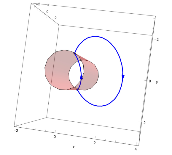
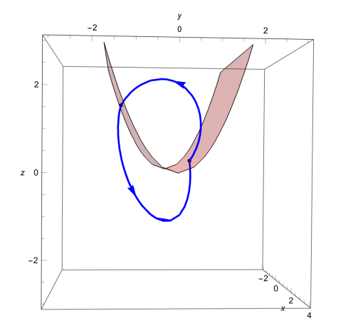
These points are classified as crossing points, since \[\begin{array}{ll} X^{+}(M_1) X^{-}(M_1)= (-0.58662, -1.723, -2.241) (0.37786, -0.40705, -0.9874)=2.6937.\\ X^{+}(N_1)X^{-}(N_1)=(0.20885, -1.5224, 0.42975)(-0.5761,-1.2971, 0.036223)=1.87003, \end{array}\] with \(X^{+}\equiv (3)\) and \(X^{-}\equiv (4)\). Therefore, the 3D-discontinuous piecewise differential system (3)-(4) separated by \(\mathcal{C}_1\) has exactly one crossing limit cycle, see Figure 1.
Retaining the same switching manifold \(\mathcal{C}_1\), we define the relay system for \(x>0\) and its first integrals in the region \(\mathcal{R}^1_1\) by choosing \[(a_{i},b_{i}, c_{i})\rightarrow \bigg(-\dfrac{711467}{11257},-\dfrac{59919}{1000},-\dfrac{3798672}{32869},\dfrac{1522033}{10000}, \dfrac{11}{5}, -2e, 1, -3, 2 \pi, 3, \sqrt{3}, -\dfrac{87}{10}\bigg),\] where \(i=1,\cdots,4\), \(e\approx 2.718281828\cdots.\) is Euler’s number and \(\pi\approx 3.14159…\).
In the region \(\mathcal{R}^1_2\) we consider the following parameters \[\begin{array}{lll} (\alpha_{i},\beta_{i}, \delta_{i} )\rightarrow &\bigg( \dfrac{1}{10}, \dfrac{43}{10}, \dfrac{143}{50}, -\dfrac{1127}{13848},\dfrac{19}{5487}, \dfrac{19}{10}, \dfrac{-29}{10}, \dfrac{1}{10} , -\dfrac{56919}{1000},-\dfrac{56919}{1000},\notag-\dfrac{56919}{500},\\ &\dfrac{1435033}{10000}\bigg), \end{array}\] where \(i=1,\cdots,4\), to obtain the linear differential center with its first integrals. For these systems, we find two real solutions that satisfy system (6) with an absolute tolerance of \(10^{-14}\). \[\begin{aligned} (M_1,N_1)= (x_1, y_1, z_1, x_{11}, y_{11}, z_{11})=& \left( \dfrac{3101}{10971},-\dfrac{65629}{68419},\dfrac{11855}{17224},\dfrac{5461}{22923},\dfrac{14606}{15039},-\dfrac{3656}{14353}\right), \notag\\ (M_2,N_2)= (x_{2}, y_{2}, z_{2}, x_{22}, y_{22}, z_{22})=& \left( \dfrac{7794}{13285},-\dfrac{23467}{28978},\dfrac{57978}{60295},\dfrac{11116}{21325},\dfrac{151649}{177701},\dfrac{4226}{25979}.\right). \end{aligned}\]
The vector fields (3) and (4) have a positive scalar product in the points \((M_i,N_i)\) with \(i=1,2\) such that;
\(\begin{array}{ll} X^{+}(M_1) X^{-}(M_1)= (-1.0981, 1.1358, -0.01883) (-2.1785, 0.2857, 0.9464)=2.69908,\\ X^{+}(N_1)X^{-}(N_1)=(1.0467, 1.0966, -1.0716)(2.1703,0.070315, -1.1203)=3.54966,\\ X^{+}(M_2) X^{-}(M_2)= (-0.95082,0.70097, 0.12492) (-1.8918, 0.59548, 0.64817)=2.2972,\\ X^{+}(N_2)X^{-}(N_2)=(0.89605, 0.6916, -0.79386)(1.8518, 0.42209,-1.1369)=2.85387. \end{array}\)
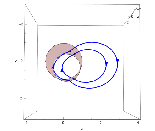
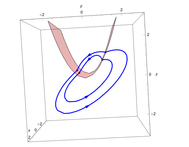
Consequently, the discontinuous piecewise differential system (3)-(4) has exactly two crossing limit cycles. This result is presented in Figure 2.
Now we build an example of three limit cycles. In the region \(\mathcal{R}_1^1\) and for \(x>0\), the relay system is characterized by the following parameters \[(a_{i},b_i, c_i)\rightarrow \left( 6, -3, 3, 0, \dfrac{43}{10}, -3, \dfrac{21}{10}, \dfrac{29}{5}, -3, 5, 2, \dfrac{29}{5} \right), \text{ with } i=1\cdots 4.\]
In the region \(\mathcal{R}_2^1\) for the linear differential center we consider the parameters \[\begin{array}{lll} (\alpha_{i},\beta_{i}, \delta_{i} )\rightarrow &\bigg( \dfrac{3}{2},2,\dfrac{1}{10},-\dfrac{13909}{34287},-\dfrac{27}{10},\dfrac{6}{5},-\dfrac{9001}{28206},\dfrac{21052}{26295},\dfrac{165879}{37768},\dfrac{55293}{18884},\notag \dfrac{109223}{14921},4 \bigg),\end{array}\] where \(i=1,\cdots,4\). According to these systems, we have three real solutions that fulfill system (6) within an absolute tolerance \(10^{-14}\), given by \[\begin{aligned} (M_1,N_1)=(x_1, y_1, z_1, x_{11}, y_{11}, z_{11})=&\left(\dfrac{253}{1649},-\dfrac{31381}{31757},\dfrac{24887}{27554},\dfrac{6415}{31278},\dfrac{7919}{8091},\dfrac{2707}{31681}\right),\notag\\ (M_2,N_2)= (x_{2}, y_{2}, z_{2}, x_{22}, y_{22}, z_{22})=&\left( \dfrac{17922}{44551},-\dfrac{27991}{30574},-\dfrac{2219}{29523},\dfrac{4553}{9095},\dfrac{29768}{34387},-\dfrac{39669}{46855}\right),\notag\\ (M_3,N_3)= (x_{3}, y_{3}, z_{3}, x_{33}, y_{33}, z_{33})=&\left(\dfrac{11261}{39301},-\dfrac{30847}{32197},\dfrac{12635}{30719},\dfrac{3608}{10033},\dfrac{26557}{28461},-\dfrac{5238}{13465}\right). \end{aligned}\]
These points correspond to a crossing type because the vector fields on both sides of the switching manifold point in the same direction, satisfying the condition \[\begin{array}{ll} X^{+}(M_1) X^{-}(M_1)= (0.77009, -1.6112, 0.1824) (0.8031,-0.03516, -0.4678)=0.58985.\\ X^{+}(N_1)X^{-}(N_1)=(-0.8482, -1.3628, 1.0540)(-0.80722, -0.11820,0.5316)=1.40614.\\ X^{+}(M_2) X^{-}(M_2)= (0.69392, -0.89152,-0.05974) (0.7354, 0.1536, -0.5027)=0.40335.\\ X^{+}(N_2)X^{-}(N_2)=(-0.77643, -0.6030, 0.70714)(-0.71911, 0.14161, 0.3748)=0.73797.\\ X^{+}(M_3) X^{-}(M_3)= (0.7363,-1.2412, 0.05472) (0.77506, 0.07034,-0.49317)=0.45637.\\ X^{+}(N_3)X^{-}(N_3)=(-0.82189, -0.9736, 0.8826)(-0.7716, 0.019181,0.4552)=1.01735. \end{array}\]
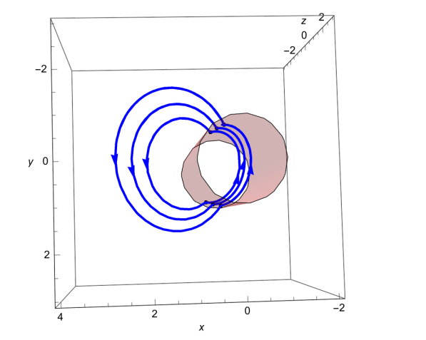
This provides exactly three crossing limit cycles for the discontinuous piecewise differential system (3)-(4) illustrated in Figure 3.
Finally, we give an example with exactly four crossing limit cycles.
In the region \(\mathcal{R}_1^1\) and for \(x>0\) we define the relay system by choosthe following parameters \[(a_i,b_i, c_i )\rightarrow \left(\dfrac{21}{5},-\dfrac{14}{5},10,1,-1,-9,6,5,-\dfrac{16}{5},3,-2,2\right), \text{ with } i=1\cdots 4.\]
In the other region \(\mathcal{R}_2^1\), for the 3D-center, we choose the following parameters \[(\alpha_i,\beta_i, \delta_i)\rightarrow \left(-\dfrac{5}{2},-2,-\dfrac{120685}{39008},\dfrac{60937}{44349},2,-4,\dfrac{55430}{9029},\dfrac{30034}{16849},\dfrac{7}{20},\dfrac{7}{100},\dfrac{14}{5},\dfrac{1}{2}\right),\] where \(i=1,\cdots,4\). The four real solutions that satisfy system (6) are \[\begin{aligned} (M_1,N_1)=(x_1, y_1, z_1, x_{11}, y_{11}, z_{11})=& \left(\dfrac{38984}{45997},-\dfrac{5516}{10393},-\dfrac{31719}{44197},\dfrac{38918}{43195},\dfrac{16407}{37817},-\dfrac{48286}{64513}\right), \notag\\ (M_2,N_2)= (x_{2}, y_{2}, z_{2}, x_{22}, y_{22}, z_{22})=& \left(\dfrac{10072}{13041},-\dfrac{11587}{18241},-\dfrac{29119}{50148},\dfrac{24493}{35139},\dfrac{40981}{57153},-\dfrac{15297}{25282}\right), \notag\\ (M_3,N_3)= (x_3, y_3, z_3, x_{33}, y_{33}, z_{33})=& \left(\dfrac{23433}{32099},-\dfrac{14887}{21783},-\dfrac{14213}{31643},\dfrac{33745}{94512},\dfrac{12471}{13351},-\dfrac{6398}{14443}\right),\notag\\ (M_4,N_4)= (x_{4}, y_{4}, z_{4}, x_{44}, y_{44}, z_{44})= & \left(\dfrac{29867}{33414},-\dfrac{12823}{28599},-\dfrac{18219}{22409},\dfrac{42311}{43461},\dfrac{13279}{58109},-\dfrac{29479}{35098}\right).\\ \end{aligned}\]
For these solutions, we have an absolute tolerance of \(10^{-13}\) and they correspond to crossing points, since
\(\begin{array}{ll} X^{+}(M_1) X^{-}(M_1)= (1.3904,-0.1709,-0.1695) (0.8827, -0.3488, -0.10162)=1.30422.\\ X^{+}(N_1)X^{-}(N_1)=(-1.3966, 0.0577, 0.17314)(-0.9248, -0.4115, 0.1258)=1.28975.\\ X^{+}(M_2) X^{-}(M_2)= (1.94319,-0.2387,-0.2369) (1.29116, -0.2211, -0.1558)=2.5987.\\ X^{+}(N_2)X^{-}(N_2)=(-1.93141, 0.0272, 0.2407)(-1.25714, -0.3897, 0.1668)=2.4576.\\ X^{+}(M_3) X^{-}(M_3)= (2.32692, -0.2824, -0.2838) (1.5969, -0.0811, -0.1975)=3.795.\\ X^{+}(N_3)X^{-}(N_3)=(-2.24631, -0.06717, 0.2824)(-1.47801, -0.4347, 0.1956)=3.40452.\\ X^{+}(M_4) X^{-}(M_4)= (0.97825, -0.1237,-0.11918) (0.9782, -0.1237, -0.1191)=0.98651.\\ X^{+}(N_4)X^{-}(N_4)=(-0.9866, 0.05209, 0.12203)(-0.9866, 0.05209,0.12203)=0.991173. \end{array}\)
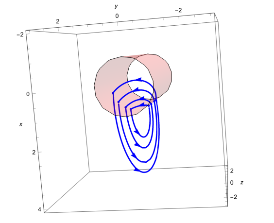
Consequently, the discontinuous piecewise differential system (3)-(4) has four crossing limit cycles; see Figure 4.
In order to prove that the second result of Theorem 1.1 is reached we build two examples with one and two limit cycles. In the region \(\mathcal{R}_1^2\) and for \(x>0\) we consider the relay system and its first integrals by choosing \[(a_{i},b_{i}, c_{i} )\rightarrow \left(\dfrac{41417}{20736},-\dfrac{1}{5},\dfrac{59455}{21308},\dfrac{17}{10},-\dfrac{3}{5},-\dfrac{8}{7},\dfrac{5}{6},-\dfrac{1}{2},-\dfrac{2}{9},\dfrac{5}{2},1,\dfrac{8}{11}\right).\]
We choose the following parameters \[(\alpha_{i},\beta_{i}, \delta_{i})\rightarrow \left(\dfrac{22}{5},\dfrac{23}{5},-3,\dfrac{89101}{41841},-2,1,-6,8,-\dfrac{2}{5},\dfrac{9}{10},\dfrac{43071}{49183},\dfrac{323269}{51630}\right),\] for the 3D-linear center in the region \(\mathcal{R}_2^2\), where \(i=1,\cdots,4\). System (12) has the unique solution \[\begin{aligned} \begin{array}{lll} (M_1,N_1)=(x_1, y_1, z_1, x_{11}, y_{11}, z_{11})= \left (\dfrac{4699}{21884},-\dfrac{13038}{9719},\dfrac{24095}{13389},\dfrac{59792}{56281},\dfrac{19889}{38131},\dfrac{5250}{19297}\right), \end{array} \end{aligned}\] with an absolute tolerance of \(10^{-14}\), and we have
\[\begin{array}{ll} X^{+}(M_1) X^{-}(M_1)= (1.8647,-0.5896, -0.5155) (1.6859, -0.07019, 0.8422)=2.75104,\\ X^{+}(N_1)X^{-}(N_1)=(-2.1232,0.0214,0.9813)(-1.6957,0.0485,-0.8245)=2.79244, \end{array}\]
namely \(M_1\) and \(N_1\) are crossing points that produce only one crossing limit cycle for the three-dimensional discontinuous piecewise differential system (3)-(4) separated by \(\mathcal{C}_2\). See Figure 5.
Now, we construct an example with exactly two crossing limit cycles. In \(\mathcal{R}_1^2\) and for \(x>0\) we consider the relay system by choosing the following parameters \[(a_{i},b_{i}, c_{i} )\rightarrow \bigg(-\dfrac{1793093}{20000},\dfrac{185677}{10000},-\dfrac{113677}{20000},\dfrac{763051}{10000},3,3,-\dfrac{17}{10},-\dfrac{277}{100},\dfrac{5}{2},\notag \dfrac{4}{5},-4,-3\bigg) .\]
In the region \(\mathcal{R}^2_2\) we take the following parameters \[\begin{aligned} ( \alpha_{i},\beta_{i}, \delta_{i}) \rightarrow& \bigg(-\dfrac{2970}{32383},\dfrac{23}{20},-\dfrac{8575}{10994},-\dfrac{11}{10},\dfrac{227}{100},-\dfrac{1}{10},\dfrac{19}{10},-\dfrac{17}{10},-\dfrac{1743093}{20000},\dfrac{193677}{10000},\notag\\ & -\dfrac{193677}{20000},\dfrac{733051}{10000}\bigg), \end{aligned}\] to obtain the 3D-center and its first integrals, where \(i=1,\cdots,4\).
For these systems, we get the two real solutions for the system (12) within an absolute tolerance of \(10^{-14}\) \[\begin{aligned} \begin{array}{lll} (M_1,N_1)=(x_1, y_1, z_1, x_{11}, y_{11}, z_{11})=& \left(\dfrac{16801}{60104},-\dfrac{14873}{25815},\dfrac{15191}{45765},\dfrac{12101}{21864},\dfrac{27087}{23821},\dfrac{62411}{48268}\right), \notag\\ (M_2,N_2)= (x_{2}, y_{2}, z_{2}, x_{22}, y_{22}, z_{22})=& \left(\dfrac{24066}{43915},-\dfrac{23004}{52519},\dfrac{8221}{42850},\dfrac{21510}{27673},\dfrac{39643}{42450},\dfrac{78014}{89453} \right). \end{array} \end{aligned}\]
The scalar product of the vector fields at the points \((M_i,N_i)\), with \(i=1,2\) equal to \[\begin{array}{ll} X^{+}(M_1) X^{-}(M_1)= (-0.2675,-2.0175, -1.6267) (0.02845,-0.4392, -1.1345)=2.7241.\\ X^{+}(N_1)X^{-}(N_1)=(-0.3634, -1.9287, -0.5869)(-0.3772,-1.7422,-0.08919)=3.549.\\ X^{+}(M_2) X^{-}(M_2)= (-0.1795, -1.3442,-1.0725) (-0.0287,-0.6028, -0.9466)=1.8308.\\ X^{+}(N_2)X^{-}(N_2)=(-0.2319,-1.11816,-0.1484)(-0.3243,-1.5102,-0.10119)=1.779. \end{array}\]
Thus, we proved the existence of two crossing limit cycles for the discontinuous piecewise differential system (3)-(4) separated by the parabolic cylinder \(\mathcal{C}_2\), see Figure 6.
Consequently, our examples confirm the result obtained in Theorem 1.1, namely; the upper bound of the maximum number of the three-dimensional crossing limit cycles of the discontinuous piecewise differential system (3)-(4) separated by one of the two cylinders \(\mathcal{C}_1\) or \(\mathcal{C}_2\) is reached.
The data sets analyzed during the current study are available from the corresponding author on reasonable request.